Weighted level set evolution based on local edge features for medical image segmentation

(1)

warwick.ac.uk/lib-publications

Original citation:

Khadidos, Alaa, Sanchez Silva, Victor and Li, Chang-Tsun. (2017) Weighted level set evolution

based on local edge features for medical image segmentation. IEEE Transactions on Image

Processing.

Permanent WRAP URL:

http://wrap.warwick.ac.uk86204

Copyright and reuse:

The Warwick Research Archive Portal (WRAP) makes this work by researchers of the

University of Warwick available open access under the following conditions. Copyright ©

and all moral rights to the version of the paper presented here belong to the individual

author(s) and/or other copyright owners. To the extent reasonable and practicable the

material made available in WRAP has been checked for eligibility before being made

available.

Copies of full items can be used for personal research or study, educational, or not-for profit

purposes without prior permission or charge. Provided that the authors, title and full

bibliographic details are credited, a hyperlink and/or URL is given for the original metadata

page and the content is not changed in any way.

Publisher’s statement:

“© 2017 IEEE. Personal use of this material is permitted. Permission from IEEE must be

obtained for all other uses, in any current or future media, including reprinting

/republishing this material for advertising or promotional purposes, creating new collective

works, for resale or redistribution to servers or lists, or reuse of any copyrighted component

of this work in other works.”

A note on versions:

The version presented here may differ from the published version or, version of record, if

you wish to cite this item you are advised to consult the publisher’s version. Please see the

‘permanent WRAP URL’ above for details on accessing the published version and note that

access may require a subscription.

(2)

JOURNAL OF LA_{TEX CLASS FILES} ₁

Weighted Level Set Evolution Based on Local Edge

Features for Medical Image Segmentation

Alaa Khadidos, Victor Sanchez,

Member, IEEE

, and Chang-Tsun Li,

Senior Member, IEEE

Abstract—Level set methods have been widely used to

imple-ment active contours for image segimple-mentation applications due to their good boundary detection accuracy. In the context of medical image segmentation, weak edges and inhomogeneities remain important issues that may hinder the accuracy of any segmentation method based on active contours implemented using level set methods. This paper proposes a method based on active contours implemented using level set methods for segmentation of such medical images. The proposed method uses a level set evolution that is based on the minimization of an objective energy functional whose energy terms are weighted according to their relative importance in detecting boundaries. This relative importance is computed based on local edge features collected from the adjacent region located inside and outside of the evolving contour. The local edge features employed are the edge intensity and the degree of alignment between the image’s gradient vector flow field and the evolving contour’s normal. We evaluate the proposed method for segmentation of various regions in real MRI and CT slices, X-ray images, and ultra sound images. Evaluation results confirm the advantage of weighting energy forces using local edge features to reduce leakage. These results also show that the proposed method leads to more accurate boundary detection results than state-of-the-art edge-based level set segmentation methods, particularly around weak edges.

Index Terms—image segmentation, medical images, active

contours, level set methods.

I. INTRODUCTION

Image segmentation is an important analysis tool in many applications of computer vision, machine learning and image analysis [1]–[13]. In medical imaging, segmentation helps extracting local information from the imaging data that can aid in clinical and diagnosis procedures [14]–[21]. State-of-the-art segmentation techniques are usually formulated as an optimization problem, where the segmentation criteria and the contour characteristics are specified by an objective functional.

Osher et al. [22] propose the level set method which

implicitly represents a curve as the zero level of the level

set, φ, of a high dimensional function. Level set methods

have been successfully used to implement active contours for segmentation applications. The basic idea is to represent contours as the level set function and to evolve the level set function according to a partial differential equation (PDE) [2], [23], [24]. This approach allows to automatically handle

Alaa Khadidos is with the Department of Computer Science, University of Warwick, Coventry CV4 7AL, UK. He is also with the Faculty of Computing and Information Technology,King Abdulaziz University, Jeddah, Saudi Arabia (e-mail: [email protected]; [email protected]).

Victor Sanchez is with the Department of Computer Science, University of Warwick, Coventry CV4 7AL, UK, (e-mail: [email protected]).

Chang-Tsun Li is with School of Computing and Mathematics, Charles Sturt University, Australia, (e-mail: [email protected]).

the topological changes of the boundary to be detected [25]. The evolution PDE of the level set function can be directly derived from the problem of minimizing a certain energy functional defined on the level set function. This type of variational methods, which are known as variational level set methods, are highly amenable to incorporating additional information in the level set evolution (LSE), such as region-based information [2], [6], shape-prior information [26] and phase-based information [19], which usually gives rise to very accurate boundary detection results.

(3)

JOURNAL OF LA_{TEX CLASS FILES} ₂

et al. [21] propose to combine an edge-based active contour model and region-based active contour model for segmentation of the left ventricle in cardiac CT images. Based on the image gradient, their method adjusts the effect of the two models. Although this method shows good performance around weak edges, the results are highly dependant on the placement of the initial contour. Ji et al.[20] propose a local region-based active contour model for medical image segmentation that uses the spatially varying mean and variance of local intensities to construct a local likelihood image fitting (LLIF) energy functional. Their method performs well in images with low contrast and intensity inhomogeneities. However, as with other region-based active contour models, it assumes the existence of two well-differentiated regions, which may not always be true in medical images.

Motivated by our previous work [45], we propose a segmen-tation method that employs an active contour implemented using a variational level set method that weights the level set evolution according to local edge features in order to accurately drive the motion of the zero level set towards the desired boundary. Specifically, our method controls the influence of energy terms in the objective functional with a weighting function that takes into account two local edge features: edge intensities and edge orientations. We employ the gradient vector flow (GVF) field of the image [46] as a measurement of local edge orientations.

Although previously proposed methods also employ local features to control the contour’s evolution [8], [21], [47], [48], they usually achieve this by incorporating additional energy terms and employing a set of empirically selected parameters to specify the influence of these terms. This may lead to inaccurate segmentation results, especially around weak edges. Other methods not based on level set methods employ edge information to balance the linear combination of energy terms in graph cut segmentation, as in [49]. In this work, instead of incorporating additional energy terms, our method employs a weighting approach to determine the effect of the two basic energy terms usually employed in edge-based active

contours implemented using level-set methods: the area and

lengthterms. Specifically, the novelties of our approach are as follows:

1) Our method measures the alignment between the evolv-ing contour’s normal direction of movement and the image’s gradient in the adjacent region located inside and outside of the evolving contour. Other methods that also measure this alignment, e.g., [29], [31], usually do this only in the adjacent region of the evolving contour in the direction of movement. Moreover, this measurement is often used as an additional energy term in the energy functional.

2) Our method also considers the average edge intensity in the adjacent region located inside and outside of the evolving contour. This allows to minimize the negative effect of weak edges on the segmentation accuracy. 3) Our method uses all of the collected local edge

informa-tion to compute a single value that serves as a weight to control the influence of forces associated with two basic energy terms: theareaandlengthterms. This minimizes

leakage in areas where weak edges exist.

We test the performance of the proposed method on a great variety of challenging medical images from MRI and CT sequences featuring weak edges and intensity inhomogeneities, as well as X-ray and ultra sound images. We compare our method’s performance to that of state-of-the-art edge-based level-set approaches, specifically, reinitialization-free level set evolution via reaction diffusion (RD) [32], active contours based on gradient vector interaction and constrained level set diffusion (LSD) [8], distance regularized level set evolution (DRLSE) [13]. We also compare our method to PBLS [19] and Kimmel’s method [29]. Results show that our proposed method attains a high boundary detection accuracy, particu-larly in areas prone to leakage.

The rest of the paper is organized as follows. Section II details our proposed method. Extensive experimental results for segmentation of real medical images are presented Section III. Section IV concludes this paper.

II. WEIGHTEDLEVELSETEVOLUTION

For medical image segmentation applications based on ac-tive contours implemented using variational level set methods, a variety of image information, such as intensity, edge or texture, can be used to define an objective functional. Here, we employ edge information as the main image feature that drives the evolving contour to the desired boundary. We use the following edge indicator function to acquire information about the intensities of edges:

g, 1

1 +_|∇Gσ∗I|

2 (1)

where g _∈ [0,1], I is an image on a domain Ω, Gσ is a

Gaussian kernel with a standard deviationσ, and _∗denotes a

convolution operation. Functiongusually takes smaller values

at object boundaries than at smooth regions. Based ong, we

define the following basic energy functional for an Level Set Function (LSF),φ:

E(φ) =R(φ) +Length(φ) +Area(φ) (2)

where R(φ) is a distance regularization term as introduced

in [13], andLength(φ)andArea(φ)are the length and area

energy terms, respectively. TermR(φ)is employed to maintain

a desired shape of the LSF, as it has been previously shown that the LSF usually becomes too flat or too steep near the zero level set, resulting in numerical errors which may eventually affect the stability of the evolution [13], [32], [50], [51]. Term

Length(φ) is related to the energy along the length of the evolving contourC, i.e., for the case whereφ=0; while term

Area(φ)is related to the energy of the area inside ofC, i.e., for the case where φ >=0. These two energy terms can be

defined so that the overall energy is minimized at the desired boundaries according to the edge indicator in Eq. (1):

Length{φ= 0}=

Z

Ω

(4)

JOURNAL OF LA_{TEX CLASS FILES} ₃

and

Area_{φ_≥0_}=

Z

Ω

gH(φ)dx (4)

where H is the Heaviside function. Note that according to

Eq. (3)-(4), the minimization of the these two energy terms depends heavily on the amount of edge information in the image. The Dirac delta functionδin Eq. (3) is used to compute

a line integral of the edge indicator functiong along the zero

level set of φ. The Heaviside function in Eq. (4), on the

other hand, is used to compute the energy of the area inside the evolving contour, C.Length(φ)is then minimized when

the zero level set of φ is located at the object’s boundary,

whileArea(φ)serves as a way to control the evolution speed

of the zero level set. In smooth regions, Area(φ) speeds

up the evolution. In regions with a high number of edges,

Area(φ) slows down the evolution, which helps the contour to conform to the desired boundary. For cases in which the image comprises smooth regions delimited by strong edges, the minimization of the energy functional in Eq. (2) provides excellent boundary detection results. However, for cases where the image comprises regions with intensity inhomogeneities or delimited by weak edges, such as in medical images, the evolution process may result in an inaccurate boundary detection or leakages. In this work, we are interested in improving the accuracy of the evolution process in conforming to the desired boundaries in cases where edges are weak, and regions contain intensity inhomogeneities. To this end, we propose a weighting function to assign different priorities to the area and length terms according to the image features of

the adjacent region located inside and outside of C. These

features are the average edge intensity, denoted by I, and

average difference between the direction of the image’s GVF

and the normal direction of movement of C, denoted by γ.

Note that analyzing the adjacent region located both inside and outside ofC, provides an accurate insight of the location of edges, which helps the zero level set to accurately conform to the desired boundary [45].

Our proposed length and area terms then include a weight-ing factor,ω, that determines their importance in locating the

desired boundary according to local edge features. These terms are defined as:

Length2{φ= 0}=

Z

Ω

g(1₋ω(φ, k))δ(φ)_|∇φ_|dx (5) and

Area2{φ≥0}=

Z

Ω

gω(φ, k)H(φ)dx (6)

where k is a constant that determines the size of the region

adjacent to C from where local edge features are obtained.

Weightω(φ, k)is given by:

ω(φ, k) =I(φ, k)(1−γ(φ,k)) (7)

whereI ∈[0,1]is the average intensity of the edge indicator

along 2k contours adjacent to C; γ _∈ [₋1,1] is the inner product between the normal ofC, denoted byN~ =∇φ/|∇φ|, and the GVF field along2kcontours adjacent toC. A contour

adjacent toC is defined as follows:

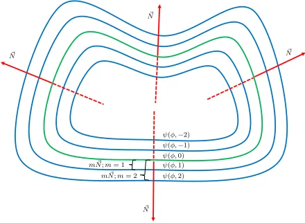
ψ(φ, m) =δ(φ)_|∇φ_|+m ~N (8)

wherem _∈Zand its sign denotes if the adjacent contour is

located outside (+) or inside (₋) ofC. Note that with the Dirac

delta function, the term m ~N in Eq. (8) results in a contour

displaced from the zero level set ofφbymunits in its normal

direction. This is illustrated in Fig. 1.1 intro

m ~N;m= 1

m ~N;m= 2

ψ(φ,−2)

ψ(φ,−1)

ψ(φ,0)

ψ(φ,1)

ψ(φ,2)

~ N ~

N

~ N

Figure 1: The red arrow represents the direction of the normal vector of con-tourC. Black arrows represent the GVF field vectors along those points in 2k

surrounding contours, withk= 2, intersected by the normal vector.

[image:4.612.327.547.181.342.2]

1

Fig. 1. The green line represents the evolving contourC, i.e., the zero level set ψ(φ,0). The blue lines represent the adjacent contours form= 1,m=−1, m= 2andm=−2, as specified in Eq. (8)

The average intensity of the edge indicator along the 2k

adjacent contours is calculated as follows:

I(φ, k) = 1

2k

k

X

m=1

" Z

Ω

(1−g)ψ(φ, m)dx

+

Z

Ω

(1₋g)ψ(φ,₋m)dx

#

(9)

Similarly to the length term in Eq. (3), the integral in Eq. (9) computes the line integral of the function(1₋g)along two contours adjacent to C; the first one located k units from C

in its outside region, and the second one locatedk units from Cin its inside region. Note that in Eq. (9), we use the inverse

value of the edge indicatorg, i.e.,(1₋g), as we are interested

in determining if the2kadjacent contours are located in areas

with strong edge information.

We observe that the direction of the image’s GVF field is a good estimator of the orientation and direction of edges [29]. Based on this observation, we calculate the alignment between the normal vector ofCand the GVF field along the2kadjacent contours, as illustrated in Fig. 2. The average inner productγ

is then calculated as follows:

γ(φ, k) = 1

2k

k

X

m=1

" Z

Ω

D ~

N , ~VEψ(φ, m)dx

+

Z

Ω

D ~

N , ~VEψ(φ,−m)dx #

(5)

JOURNAL OF LA_{TEX CLASS FILES} ₄

where _V~ _{denotes the image’s GVF field. In this case, the}

integral in Eq. (10) computes the line integral of the inner product between _N~ _and_V~ _{along the contours adjacent to} _C_.

Note thatγresults in values close to 1 when the normal vector of ↑ ↑ ↑ ↑ ↑ ↑ ↑ ↑ ↑ ↑ ↑ ↑ ↑ ↑ ↑ ↑ ↑ ↑ ↑ ↑ ↑ ↑ ↑ ↑ ↑ ↑ ↑ ↑ C aligns with_V~_.

↑ ↑ ↑ ↑ ↑ ↑ ↑ ↑ ↑ ↑ ↑ ↑ ↑ ↑ ↑ ↑ ↑ ↑ ↑ ↑ ↑ ↑ ↑ ↑ ↑ ↑ ↑ ↑ ↖ ↑ ↑ ↑ ↑ ↑ ↑ ↑ ↑ ↑ ↑ ↑ ↑ ↑ ↑ ↑ ↑ ↑ ↑ ↑ ↑ ↑ ↑ ↑ ↑ ↑ ↑ ↗ ↖ ↖ ↑ ↑ ↑ ↑ ↑ ↑ ↑ ↑ ↑ ↑ ↑ ↑ ↑ ↑ ↑ ↑ ↑ ↑ ↑ ↑ ↑ ↑ ↑ ↑ ↑ ↗ ↖ ↖ ↑ ↑ ↑ ↑ ↑ ↑ ↑ ↑ ↑ ↑ ↑ ↑ ↑ ↑ ↑ ↑ ↑ ↑ ↑ ↑ ↑ ↑ ↑ ↑ ↗ ↗ ↖ ↖ ↖ ↑ ↑ ↑ ↑ ↑ ↑ ↑ ↑ ↑ ↑ ↑ ↑ ↑ ↑ ↑ ↑ ↑ ↑ ↑ ↑ ↑ ↑ ↗ ↗ ↗ ↖ ↖ ↖ ↖ ↑ ↑ ↑ ↑ ↑ ↑ ↑ ↑ ↑ ↑ ↑ ↑ ↑ ↑ ↑ ↑ ↑ ↑ ↑ ↑ ↑ ↗ ↗ ↗ ↗ ↗ ↗ ↖ ↖ ↖ ↖ ↖ ↑ ↑ ↑ ↑ ↑ ↑ ↑ ↑ ↑ ↑ ↑ ↑ ↑ ↑ ↑ ↑ ↑ ↑ ↑ ↑ ↗ ↗ ↗ ↗ ↗ ↗ ↖ ↖ ↖ ↖ ↑ ↑ ↑ ↑ ↑ ↑ ↑ ↑ ↑ ↑ ↑ ↑ ↑ ↑ ↑ ↑ ↑ ↑ ↑ ↑ ↗ ↗ ↗ ↗ ↗ ↗ ↖ ↖ ↖ ↖ ↖ ↑ ↑ ↑ ↑ ↑ ↑ ↑ ↑ ↑ ↑ ↑ ↑ ↑ ↑ ↑ ↑ ↑ ↑ ↑ ↗ ↗ ↗ ↗ ↗ ↗ ↗ ↖ ↖ ↖ ↖ ↖ ↖ ↑ ↑ ↑ ↑ ↑ ↑ ↑ ↑ ↑ ↑ ↑ ↑ ↑ ↑ ↑ ↑ ↑ ↗ ↗ ↗ ↗ ↗ ↗ ↗ ↗ ↖ ↖ ↖ ↖ ↖ ↖ ↑ ↑ ↑ ↑ ↑ ↑ ↑ ↑ ↑ ↑ ↑ ↑ ↑ ↑ ↑ ↑ ↗ ↗ ↗ ↗ ↗ ↗ ↗ ↗ ↗ ↖ ↖ ↖ ↖ ↖ ↖ ↖ ↖ ↖ ↖ ↖ ↑ ↑ ↑ ↑ ↑ ↑ ↑ ↑ ↑ ↑ ↗ ↗ ↗ ↗ ↗ ↗ ↗ ↗ ↗ ↗ ↖ ↖ ↖ ↖ ↖ ↖ ↖ ↖ ↖ ↖ ↖ ↑ ↑ ↑ ↑ ↑ ↑ ↑ ↗ ↑ ↗ ↗ ↗ ↗ ↗ ↗ ↗ ↗ ↗ ↗ ↗ ↖ ↖ ↖ ↖ ↖ ↖ ↖ ↖ ↖ ↖ ↖ ↑ ↑ ↑ ↑ ↑ ↑ ↗ ↗ ↗ ↗ ↗ ↗ ↗ ↗ ↗ ↗ ↗ ↗ ↗ ↗ ↖ ↖ ↖ ↖ ↖ ↖ ↖ ↖ ↖ ↖ ↖ ↑ ↑ ↑ ↑ ↑ ↑ ↗ ↗ ↗ ↗ ↗ ↗ ↗ ↗ ↗ ↗ ↗ ↗ ↗ ↗ ↖ ↖ ↖ ↖ ↖ ↖ ↖ ↖ ↖ ↖ ↖ ↑ ↑ ↑ ↑ ↗ ↗ → → ↗ ↗ ↗ ↗ ↗ ↗ ↗ ↗ ↗ ↗ ↗ ↗ ↖ ↖ ↖ ↖ ↖ ↖ ↖ ↖ ↖ ↖ ↖ ← ← ↑ ↑ → → → → ↗ ↗ ↗ ↗ ↗ ↗ ↗ ↗ ↗ ↗ ↗ ↗ ↖ ↖ ↖ ↖ ↖ ↖ ↖ ← ← ← ← ← ← ↓ ↓ → → → → ↗ ↗ ↗ ↗ ↗ ↗ ↗ ↗ ↗ ↗ ↗ ↗ ↖ ↖ ↖ ↖ ↖ ↖ ↖ ← ← ← ← ← ↓ ↓ ↓ → → → → ↗ ↗ ↗ ↗ ↗ ↗ ↗ ↗ ↗ ↗ ↗ ↗ ← ← ← ← ← ← ← ← ↙ ↙ ↙ ← ↓ ↓ ↓ ↓ ↘ → → → → → → → → ↗ ↗ ↗ ↗ ↗ ↗ ↙ ↙ ↙ ↙ ↙ ↙ ↙ ↙ ↙ ↙ ↙ ↙ ↓ ↓ ↓ ↓ ↓ ↘ ↘ ↘ ↘ ↘ ↘ ↘ ↘ ↘ ↘ ↘ ↗ ↗ ↗ ↙ ↙ ↙ ↙ ↙ ↙ ↙ ↙ ↙ ↙ ↓ ↓ ↓ ↓ ↓ ↓ ↓ ↓ ↓ ↘ ↘ ↘ ↘ ↘ ↘ ↘ ↘ ↘ ↗ ↗ ↗ ↙ ↙ ↙ ↙ ↙ ↙ ↙ ↙ ↙ ↙ ↓ ↓ ↓ ↓ ↓ ↓ ↓ ↓ ↓ ↘ ↘ ↘ ↘ ↘ ↘ ↘ ↘ ↘ ↗ ↗ ↗ ↙ ↙ ↙ ↙ ↙ ↙ ↙ ↙ ↙ ↙ ↓ ↓ ↓ ↓ ↓ ↓ ↓ ↓ ↓ ↘ ↘ ↘ ↘ ↘ ↘ ↘ ↘ ↘ ↗ ↗ ↗ ↙ ↙ ↙ ↙ ↙ ↙ ↙ ↙ ↙ ↓ ↓ ↓ ↓ ↓ ↓ ↓ ↓ ↓ ↓ ↘ ↘ ↘ ↘ ↘ ↘ ↘ ↘ ↘ ↙ ↙ ↙ ↙ ↙ ↙ ↙ ↙ ↙ ↓ ↓ ↓ ↓ ↓ ↓ ↓ ↓ ↓ ↓ ↘ ↘ ↘ ↘ ↘ ↘ ↘ ↘ ↘ ↙ ↙ ↙ ↙ ↙ ↙ ↙ ↙ ↙ ↓ ↓ ↓ ↓ ↓ ↓ ↓ ↓ ↓ ↓ ↘ ↘ ↘ ↘ ↘ ↘ ↘ ↘ ↘ ↙ ↙ ↙ ↙ ↙ ↙ ↙ ↙ ↙ ↓ ↓ ↓ ↓ ↓ ↓ ↓ ↓ ↓ ↓ ↘ ↘ ↘ ↘ ↘ ↘ ↘ ↘ ↘ ↙ ↙ ↙ ↙ ↙ ↙ ↙ ↙ ↙ ↓ ↓ ↓ ↓ ↓ ↓ ↓ ↓ ↓ ↓ ↘ ↘ ↘ ↘ ↘ ↘ ↘ ↘ ↘ ↙ ↙ ↙ ↙ ↙ ↙ ↙ ↙ ↙ ↓ ↓ ↓ ↓ ↓ ↓ ↓ ↓ ↓ ↓ ↓ ↘ ↘ ↘ ↘ ↘ ↘ ↘ ↘ ↙ ↙ ↙ ↙ ↙ ↙ ↙ ↙ ↙ ↓ ↓ ↓ ↓ ↓ ↓ ↓ ↓ ↓ ↓ ↓ ↘ ↘ ↘ ↘ ↘ ↘ ↘ ↘ ↙ ↙ ↙ ↙ ↙ ↙ ↙ ↙ ↙ ↓ ↓ ↓ ↓ ↓ ↓ ↓ ↓ ↓ ↓ ↓ ↓ ↓ ↘ ↘ ↘ ↘ ↘ ↘

ψ(φ,−2)

ψ(φ,−1)

ψ(φ,0)

ψ(φ,1)

ψ(φ,2)

~ N ~

N

~ N

Figure 1: The red arrow represents the direction of the normal vector of con-tourC. Black arrows represent the GVF field vectors along those points in 2k

surrounding contours, withk= 2, intersected by the normal vector.

1 intro

1

Fig. 2. The red arrow represents the normal direction of movement of the evolving contour C. Gray arrows represent the GVF field vectors,_V~_{. The} figure shows the case ofk= 2.

By replacing Length(φ) and Area(φ) in Eq. (2) with

Length2(φ)andArea2(φ)as formulated in Eq. (5) and (6),

respectively, our proposed energy functional is then defined as:

E(φ) =µ Z

Ω

p(_|∇φ_|)dx+ (1₋ω(φ, k))

Z

Ω

gδ(φ)_|∇φ_|dx

+(ω(φ, k))

Z

Ω

gH(φ)dx

(11) whereµ >0is a constant, andp(s),1

2(s−1)

2

is a potential (or energy density) function with a minimum point s= 1that minimizes the distance regularization termRwhen|∇φ_|= 1

[13]. The energy functional in Eq. (11) can then be minimized by solving a gradient flow as follows:

∂φ

∂t =µdiv(dp(|∇φ|)∇φ)

+(1₋ω(φ, k))δ(φ)div(g ∇φ

|∇φ|) +ω(φ, k)gδ(φ)

(12) where dp is a function defined using the first derivative of

p(s) as dp(s) , p 0₍_s₎

s [13]. It is important to mention that

in Eq. (12), the weighting term ω(φ, k), although expressed as a function of φ and k, results in a constant value in the range [0,1]. Consequently, it is regarded as a constant when

computing the partial derivative with respect to time t. The

weighting function ω(φ, k) assigns different priorities to the

length and area terms according to local edge features. These features are the edge intensity,I, and the degree of alignment,

γ, betweenV~ andC’s normal direction of movement. Fig. 3

shows the plot ofω(φ, k)for various values ofIandγ. It can

be seen that ω approaches 0 for largeI values regardless of

the value ofγ, i.e., when the zero level set is located in a non-smooth region. In this case, theLength2term acts as the main

0 0.1 0.2 0.3 0.4 0.5 0.6 0.7 0.8 0.9 1

ω

I

γ=-1 γ=-0.9 γ=-0.8 γ=-0.7 γ=-0.6 γ=-0.5 γ=-0.4 γ=-0.3 γ=-0.2 γ=-0.1 γ=0 γ=0.1 γ=0.2 γ=0.3 γ=0.4 γ=0.5 γ=0.6 γ=0.7 γ=0.8 γ=0.9 γ=1

Fig. 3. Value ofωfor different values ofIandγ.

energy driving the zero level set to the object’s boundary. It can also be seen thatω approaches 1 for smallIvalues regardless of the value ofγ. In this case, theArea2term acts as the main

energy driving the zero level set towards the object’s boundary within a smooth region. For values ofγ close to 1, the value ofω slowly decreases asI increases. In this case, the normal

direction of movement of C aligns with the direction of the

image’s GVF field, therefore theArea2 term acts as the main

energy term. For values ofγclose to -1, the value ofωslowly

decreases asI increases. In this case, the normal direction of movement ofCis opposite to the direction of the image’s GVF

field, therefore theLength2term acts as the main energy term

helpingC to conform to the object’s boundary.

Weight ω allows C to deform in relatively smooth areas

even if its normal direction of movement is opposite to the GVF field surrounding C. This is particularly useful to

initialize the contour far from the desired boundary, even in regions with intensity inhomogeneities. Fig. 4(a)-(b) illustrate

this case, where ω approaches 1. Weight ω also minimizes

leakages around weak edges by determining the influence of the energy terms in the evolution process according to the average intensities of edge information and the average direction of the GVF field in the inside and outside regions adjacent toC. This is illustrated in Fig. 4(c), where the value

of ω slowly approaches 0. Finally, weight ω allows C to

conform to the desired boundary by assigning a larger weight

to the Length2 term where strong edges are encountered in

the inside and outside regions adjacent toC. This is illustrated

in Fig. 4(d), where the value ofω approaches 1.

III. EXPERIMENTALRESULTS

[image:5.612.63.286.123.293.2]

(6)

JOURNAL OF LA_{TEX CLASS FILES} ₅ ↑ ↑ ↑ ↑ ↑ ↑ ↑ ↑ ↑ ↑ ↑ ↑ ↑ ↑ ↑ ↑ ↑ ↑ ↑ ↑ ↑ ↑ ↑ ↑ ↑ ↑ ↑ ↑ ↑ ↑ ↑ ↑ ↑ ↑ ↑ ↑ ↑ ↑ ↑ ↑ ↑ ↑ ↑ ↑ ↑ ↑ ↑ ↑ ↑ ↑ ↑ ↑ ↑ ↑ ↑ ↑ ↑ ↑ ↑ ↑ ↑ ↑ ↑ ↑ ↑ ↑ ↑ ↑ ↑ ↑ ↑ ↑ ↑ ↑ ↑ ↑ ↑ ↑ ↑ ↑ ↑ ↑ ↑ ↑ ↑ ↑ ↑ ↑ ↑ ↑ ↑ ↑ ↑ ↑ ↑ ↑ ↑ ↑ ↑ ↑ ↑ ↑ ↑ ↑ ↑ ↑ ↑ ↑ ↑ ↑ ↑ ↑ ↑ ↑ ↑ ↑ ↑ ↑ ↑ ↑ ↑ ↑ ↑ ↑ ↑ ↑ ↑ ↑ ↑ ↑ ↑ ↑ ↑ ↑ ↑ ↑ ↑ ↑ ↑ ↑ ↑ ↑ ↑ ↑ ↑ ↑ ↑ ↑ ↑ ↑ ↑ ↑ ↑ ↑ ↑ ↑ ↑ ↑ ↑ ↑ ↑ ↑ ↑ ↑ ↑ ↑ ↑ ↑ ↑ ↑ ↑ ↑ ↑ ↑ ↑ ↑ ↑ ↑ ↑ ↑ ↑ ↑ ↑ ↑ ↑ ↑ ↑ ↑ ↑ ↑ ↑ ↑ ↑ ↑ ↑ ↑ ↗ ↗ ↗ ↑ ↑ ↑ ↑ ↑ ↑ ↑ ↑ ↑ ↑ ↑ ↑ ↑ ↑ ↑ ↑ ↑ ↑ ↑ ↑ ↑ ↑ ↑ ↑ ↑ ↑ ↑ ↑ ↗ ↗ ↗ ↑ ↑ ↑ ↑ ↑ ↑ ↑ ↑ ↑ ↑ ↑ ↑ ↑ ↑ ↑ ↑ ↑ ↑ ↑ ↑ ↑ ↑ ↑ ↑ ↑ ↑ ↑ ↑ ↗ ↗ ↗ ↑ ↑ ↑ ↑ ↑ ↑ ↑ ↑ ↑ ↑ ↑ ↑ ↑ ↑ ↑ ↑ ↑ ↑ ↑ ↑ ↑ ↑ ↑ ↑ ↑ ↑ ↑ ↑ ↗ ↗ ↗ ↑ ↑ ↑ ↑ ↑ ↑ ↑ ↑ ↑ ↑ ↑ ↑ ↑ ↑ ↑ ↑ ↑ ↑ ↑ ↑ ↑ ↑ ↑ ↑ ↑ ↑ ↑ ↑ ↗ ↗ ↗ ↑ ↑ ↑ ↑ ↑ ↑ ↑ ↑ ↑ ↑ ↑ ↑ ↑ ↑ ↑ ↑ ↑ ↑ ↑ ↑ ↑ ↑ ↑ ↑ ↑ ↑ ↑ ↑ ↗ ↗ ↗ ↑ ↑ ↑ ↑ ↑ ↑ ↑ ↑ ↑ ↑ ↑ ↑ ↑ ↑ ↑ ↑ ↑ ↑ ↑ ↑ ↑ ↑ ↑ ↑ ↑ ↑ ↑ ↑ ↗ ↗ ↗ ↑ ↑ ↑ ↑ ↑ ↑ ↑ ↑ ↑ ↑ ↑ ↑ ↑ ↑ ↑ ↑ ↑ ↑ ↑ ↑ ↑ ↑ ↑ ↑ ↑ ↑ ↑ ↑ ↗ ↗ ↗ ↑ ↑ ↑ ↑ ↑ ↑ ↑ ↑ ↑ ↑ ↑ ↑ ↑ ↑ ↑ ↑ ↑ ↑ ↑ ↑ ↑ ↑ ↑ ↑ ↑ ↑ ↑ ↑ ↗ ↗ ↗ ↑ ↑ ↑ ↑ ↑ ↑ ↑ ↑ ↑ ↑ ↑ ↑ ↑ ↑ ↑ ↑ ↑ ↑ ↑ ↑ ↑ ↑ ↑ ↑ ↑ ↑ ↑ ↑ ↗ ↗ ↗ ↑ ↑ ↑ ↑ ↑ ↑ ↑ ↑ ↑ ↑ ↑ ↑ ↑ ↑ ↑ ↑ ↑ ↑ ↑ ↑ ↑ ↑ ↑ ↑ ↑ ↑ ↑ ↑ ↗ ↗ ↗ ↑ ↑ ↑ ↑ ↑ ↑ ↑ ↑ ↑ ↑ ↑ ↑ ↑ ↑ ↑ ↑ ↑ ↑ ↑ ↑ ↑ ↑ ↑ ↑ ↑ ↑ ↑ ↑ ↗ ↗ ↗ ↑ ↑ ↑ ↑ ↑ ↑ ↑ ↑ ↑ ↑ ↑ ↑ ↑ ↑ ↑ ↑ ↑ ↑ ↑ ↑ ↑ ↑ ↑ ↑ ↑ ↑ ↑ ↑ ↗ ↗ ↗ ↑ ↑ ↑ ↑ ↑ ↑ ↑ ↑ ↑ ↑ ↑ ↑ ↑ ↑ ↑ ↑ ↑ ↑ ↑ ↑ ↑ ↑ ↑ ↑ ↑ ↑ ↑ ↑ ↗ ↗ ↗ ↑ ↑ ↑ ↑ ↑ ↑ ↑ ↑ ↑ ↑ ↑ ↑ ↑ ↑ ↑ ↑ ↑ ↑ ↑ ↑ ↑ ↑ ↑ ↑ ↑ ↑ ↑ ↑ ↗ ↗ ↗ ↑ ↑ ↑ ↑ ↑ ↑ ↑ ↑ ↑ ↑ ↑ ↑ ↑ ↑ ↑ ↑ ↑ ↑ ↑ ↑ ↑ ↑ ↑ ↑ ↑ ↑ ↑ ↑ ↗ ↗ ↗ ↑ ↑ ↑ ↑ ↑ ↑ ↑ ↑ ↑ ↑ ↑ ↑ ↑ ↑ ↑ ↑ ↑ ↑ ↑ ↑ ↑ ↑ ↑ ↑ ↑ ↑ ↑ ↑ ↗ ↗ ↗ ↑ ↑ ↑ ↑ ↑ ↑ ↑ ↑ ↑ ↑ ↑ ↑ ↑ ↑ ↑ ↑ ↑ ↑ ↑ ↑ ↑ ↑ ↑ ↑ ↑ ↑ ↑ ↑ ↗ ↗ ↗ ↑ ↑ ↑ ↑ ↑ ↑ ↑ ↑ ↑ ↑ ↑ ↑ ↑ ↑ ↑ ↑ ↑ ↑ ↑ ↑ ↑ ↑ ↑ ↑ ↑ ↑ ↑ ↑ ↗ ↗ ↗ ↑ ↑ ↑ ↑ ↑ ↑ ↑ ↑ ↑ ↑ ↑ ↑ ↑ ↑ ↑ ↑ ↑ ↑ ↑ ↑ ↑ ↑ ↑ ↑ ↑ ↑ ↑ ↑ ↑ ↑ ↑ ↑ ↑ ↑ ↑ ↑ ↑ ↑ ↑ ↑ ↑ ↑ ↑ ↑ ↑ ↑ ↑ ↑ ↑ ↑ ↑ ↑ ↑ ↑ ↑ ↑ ↑ ↑ ↑ ↑ ↑ ↑ ↑ ↑ ↑ ↑ ↑ ↑ ↑ ↑ ↑ ↑ ↑ ↑ ↑ ↑ ↑ ↑ ↑ ↑ ↑ ↑ ↑ ↑ ↑ ↑ ↑ ↑ ↑ ↑ ↑ ↑ ↑ ↑ ↑ ↑ ↑ ↑ ↑ ↑ ↑ ↑ ↑ ↑ ↑ ↑ ↑ ↑ ↑ ↑ ↑ ↑ ↑ ↑ ↑ ↑ ↑ ↑ ↑ ↑ ↑ ↑ ↑ ↑ ↑ ↑ ↑ ↑ ↑ ↑ ↑ ↑ ↑ ↑ ↑ ↑ ↑ ↑ ↑ ↑ ↑ ↑ ↑ ↑ ↑ ↑ ↑ ↑ ↑ ↑ ↑ ↑ ↑ ↑ ↑ ↑ ↑ ↑ ↑ ↑ ↑ ↑ ↑ ↑ ↑ ↑ ↑ ↑ ↑ ↙ ↙ ↙ ↙ ↙ ↙ ↙ ↙ ↓ ↓ ↓ ↓ ↓ ↓ ↓ ↓ ↓ ↓ ↓ ↘ ↘ ↘ ↘ ↘ ↘ ↘ ↘ ↙ ↙ ↙ ↙ ↙ ↙ ↙ ↙ ↙ ↓ ↓ ↓ ↓ ↓ ↓ ↓ ↓ ↓ ↓ ↓ ↓ ↓ ↘ ↘ ↘ ↘ ↘ ↘ (a) ↓ ↓ ↓ ↓ ↓ ↓ ↓ ↓ ↓ ↓ ↓ ↓ ↓ ↓ ↓ ↓ ↓ ↓ ↓ ↓ ↓ ↓ ↓ ↓ ↓ ↓ ↓ ↓ ↓ ↓ ↓ ↓ ↓ ↓ ↓ ↓ ↓ ↓ ↓ ↓ ↓ ↓ ↓ ↓ ↓ ↓ ↓ ↓ ↓ ↓ ↓ ↓ ↓ ↓ ↓ ↓ ↓ ↓ ↓ ↓ ↓ ↓ ↓ ↓ ↓ ↓ ↓ ↓ ↓ ↓ ↓ ↓ ↓ ↓ ↓ ↓ ↓ ↓ ↓ ↓ ↓ ↓ ↓ ↓ ↓ ↓ ↓ ↓ ↓ ↓ ↓ ↓ ↓ ↓ ↓ ↓ ↓ ↓ ↓ ↓ ↓ ↓ ↓ ↓ ↓ ↓ ↓ ↓ ↓ ↓ ↓ ↓ ↓ ↓ ↓ ↓ ↓ ↓ ↓ ↓ ↓ ↓ ↓ ↓ ↓ ↓ ↓ ↓ ↓ ↓ ↓ ↓ ↓ ↓ ↓ ↓ ↓ ↓ ↓ ↓ ↓ ↓ ↓ ↓ ↓ ↓ ↓ ↓ ↓ ↓ ↓ ↓ ↓ ↓ ↓ ↓ ↓ ↓ ↓ ↓ ↓ ↓ ↓ ↓ ↓ ↓ ↓ ↓ ↓ ↓ ↓ ↓ ↓ ↓ ↓ ↓ ↓ ↓ ↓ ↓ ↓ ↓ ↓ ↓ ↓ ↓ ↓ ↓ ↓ ↓ ↓ ↓ ↓ ↓ ↓ ↓ ↓ ↓ ↓ ↓ ↓ ↓ ↓ ↓ ↓ ↓ ↓ ↓ ↓ ↓ ↗ ↓ ↓ ↓ ↓ ↓ ↓ ↓ ↓ ↓ ↓ ↓ ↓ ↓ ↓ ↓ ↓ ↓ ↓ ↓ ↓ ↓ ↓ ↓ ↓ ↓ ↓ ↓ ↓ ↓ ↓ ↗ ↓ ↓ ↓ ↓ ↓ ↓ ↓ ↓ ↓ ↓ ↓ ↓ ↓ ↓ ↓ ↓ ↓ ↓ ↓ ↓ ↓ ↓ ↓ ↓ ↓ ↓ ↓ ↓ ↓ ↓ ↗ ↓ ↓ ↓ ↓ ↓ ↓ ↓ ↓ ↓ ↓ ↓ ↓ ↓ ↓ ↓ ↓ ↓ ↓ ↓ ↓ ↓ ↓ ↓ ↓ ↓ ↓ ↓ ↓ ↓ ↓ ↗ ↓ ↓ ↓ ↓ ↓ ↓ ↓ ↓ ↓ ↓ ↓ ↓ ↓ ↓ ↓ ↓ ↓ ↓ ↓ ↓ ↓ ↓ ↓ ↓ ↓ ↓ ↓ ↓ ↓ ↓ ↗ ↓ ↓ ↓ ↓ ↓ ↓ ↓ ↓ ↓ ↓ ↓ ↓ ↓ ↓ ↓ ↓ ↓ ↓ ↓ ↓ ↓ ↓ ↓ ↓ ↓ ↓ ↓ ↓ ↓ ↓ ↗ ↓ ↓ ↓ ↓ ↓ ↓ ↓ ↓ ↓ ↓ ↓ ↓ ↓ ↓ ↓ ↓ ↓ ↓ ↓ ↓ ↓ ↓ ↓ ↓ ↓ ↓ ↓ ↓ ↓ ↓ ↗ ↓ ↓ ↓ ↓ ↓ ↓ ↓ ↓ ↓ ↓ ↓ ↓ ↓ ↓ ↓ ↓ ↓ ↓ ↓ ↓ ↓ ↓ ↓ ↓ ↓ ↓ ↓ ↓ ↓ ↓ ↗ ↓ ↓ ↓ ↓ ↓ ↓ ↓ ↓ ↓ ↓ ↓ ↓ ↓ ↓ ↓ ↓ ↓ ↓ ↓ ↓ ↓ ↓ ↓ ↓ ↓ ↓ ↓ ↓ ↓ ↓ ↗ ↓ ↓ ↓ ↓ ↓ ↓ ↓ ↓ ↓ ↓ ↓ ↓ ↓ ↓ ↓ ↓ ↓ ↓ ↓ ↓ ↓ ↓ ↓ ↓ ↓ ↓ ↓ ↓ ↓ ↓ ↗ ↓ ↓ ↓ ↓ ↓ ↓ ↓ ↓ ↓ ↓ ↓ ↓ ↓ ↓ ↓ ↓ ↓ ↓ ↓ ↓ ↓ ↓ ↓ ↓ ↓ ↓ ↓ ↓ ↓ ↓ ↗ ↓ ↓ ↓ ↓ ↓ ↓ ↓ ↓ ↓ ↓ ↓ ↓ ↓ ↓ ↓ ↓ ↓ ↓ ↓ ↓ ↓ ↓ ↓ ↓ ↓ ↓ ↓ ↓ ↓ ↓ ↗ ↓ ↓ ↓ ↓ ↓ ↓ ↓ ↓ ↓ ↓ ↓ ↓ ↓ ↓ ↓ ↓ ↓ ↓ ↓ ↓ ↓ ↓ ↓ ↓ ↓ ↓ ↓ ↓ ↓ ↓ ↗ ↓ ↓ ↓ ↓ ↓ ↓ ↓ ↓ ↓ ↓ ↓ ↓ ↓ ↓ ↓ ↓ ↓ ↓ ↓ ↓ ↓ ↓ ↓ ↓ ↓ ↓ ↓ ↓ ↓ ↓ ↗ ↓ ↓ ↓ ↓ ↓ ↓ ↓ ↓ ↓ ↓ ↓ ↓ ↓ ↓ ↓ ↓ ↓ ↓ ↓ ↓ ↓ ↓ ↓ ↓ ↓ ↓ ↓ ↓ ↓ ↓ ↗ ↓ ↓ ↓ ↓ ↓ ↓ ↓ ↓ ↓ ↓ ↓ ↓ ↓ ↓ ↓ ↓ ↓ ↓ ↓ ↓ ↓ ↓ ↓ ↓ ↓ ↓ ↓ ↓ ↓ ↓ ↗ ↓ ↓ ↓ ↓ ↓ ↓ ↓ ↓ ↓ ↓ ↓ ↓ ↓ ↓ ↓ ↓ ↓ ↓ ↓ ↓ ↓ ↓ ↓ ↓ ↓ ↓ ↓ ↓ ↓ ↓ ↗ ↓ ↓ ↓ ↓ ↓ ↓ ↓ ↓ ↓ ↓ ↓ ↓ ↓ ↓ ↓ ↓ ↓ ↓ ↓ ↓ ↓ ↓ ↓ ↓ ↓ ↓ ↓ ↓ ↓ ↓ ↗ ↓ ↓ ↓ ↓ ↓ ↓ ↓ ↓ ↓ ↓ ↓ ↓ ↓ ↓ ↓ ↓ ↓ ↓ ↓ ↓ ↓ ↓ ↓ ↓ ↓ ↓ ↓ ↓ ↓ ↓ ↗ ↓ ↓ ↓ ↓ ↓ ↓ ↓ ↓ ↓ ↓ ↓ ↓ ↓ ↓ ↓ ↓ ↓ ↓ ↓ ↓ ↓ ↓ ↓ ↓ ↓ ↓ ↓ ↓ ↓ ↓ ↓ ↓ ↓ ↓ ↓ ↓ ↓ ↓ ↓ ↓ ↓ ↓ ↓ ↓ ↓ ↓ ↓ ↓ ↓ ↓ ↓ ↓ ↓ ↓ ↓ ↓ ↓ ↓ ↓ ↓ ↓ ↓ ↓ ↓ ↓ ↓ ↓ ↓ ↓ ↓ ↓ ↓ ↓ ↓ ↓ ↓ ↓ ↓ ↓ ↓ ↓ ↓ ↓ ↓ ↓ ↓ ↓ ↓ ↓ ↓ ↓ ↓ ↓ ↓ ↓ ↓ ↓ ↓ ↓ ↓ ↓ ↓ ↓ ↓ ↓ ↓ ↓ ↓ ↓ ↓ ↓ ↓ ↓ ↓ ↓ ↓ ↓ ↓ ↓ ↓ ↓ ↓ ↓ ↓ ↓ ↓ ↓ ↓ ↓ ↓ ↓ ↓ ↓ ↓ ↓ ↓ ↓ ↓ ↓ ↓ ↓ ↓ ↓ ↓ ↓ ↓ ↓ ↓ ↓ ↓ ↓ ↓ ↓ ↓ ↓ ↓ ↓ ↓ ↓ ↓ ↓ ↓ ↓ ↓ ↓ ↓ ↓ ↓ ↓ ↓ ↓ ↓ ↓ ↓ ↓ ↓ ↓ ↓ ↓ ↓ ↓ ↓ ↓ ↓ ↓ ↓ ↓ ↓ ↓ ↓ ↓ ↓ ↓ ↓ ↓ ↓ ↓ ↓ ↓ ↓ ↓ ↓ ↓ ↓ ↓ ↓ ↓ ↓ ↓ ↓ ↓ ↓ ↓ ↓ ↓ ↓ ↓ ↓ ↓ ↓ ↓ ↓ ↓ ↓ ↓ ↓ ↓ ↓ ↓ ↓ ↓ ↓ ↓ ↓ ↓ ↓ ↓ ↓ ↓ ↓ (b) ↓ ↓ ← ↓ ↓ ↓ ↓ ↓ ↓ ↓ ↓ ↓ ↓ ↓ ↓ ↓ ↓ ↓ ↓ ↓ ↓ ↓ ↓ ↓ ↓ ↓ ↓ ↓ ↓ ↓ ↘ ↗ ↑ ↓ ↓ ↓ ↓ ↓ ↓ ↓ ↓ ↓ ↓ ↓ ↓ ↓ ↓ ↓ ↓ ↓ ↓ ↓ ↓ ↓ ↓ ↓ ↓ ↓ ↓ ↓ → ↓ ↓ ↓ ↓ ↓ ↓ ↓ ↓ ↓ ↓ ↓ ↑ ↑ ↓ ↓ ↓ ↓ ↓ ↓ ↓ ↓ ↓ ↓ ↓ ↓ ↓ ↓ ↓ ↓ ↖ ↓ ↓ ↓ ↖ ↖ ↖ ↖ ↖ ↑ ↑ ↑ ↑ ↑ ↓ ↓ ↓ ↓ ↓ ↓ ↓ ↓ ↓ ↓ ↓ ↓ ↓ ↓ ↓ ↓ ↓ ↓ ↓ ↓ ↖ ↖ ↖ ↖ ↖ ↑ ↑ ↑ ↑ ↑ ↓ ↓ ↓ ↓ ↓ ↓ ↓ ↓ ↓ ↓ ↓ ↓ ↓ ↓ ↓ ↓ ↓ ↓ ↓ ↓ ↖ ↖ ↖ ↖ ↖ ↑ ↑ ↑ ↑ ↑ ↓ ↓ ↓ ↓ ↓ ↓ ↓ ↓ ↓ ↓ ↓ ↓ ↓ ↓ ↓ ↓ ↓ ↓ ↓ ↓ ↖ ↖ ↖ ↖ ↖ ↑ ↑ ↑ ↑ ↑ ↑ ↑ ↑ ↑ ↑ ↑ ↑ ↓ ↓ ↓ ↓ ↓ ↓ ↓ ↓ ↓ ↗ ↓ ↓ ↓ ↓ ↖ ↖ ↖ ↖ ↖ ↑ ↑ ↑ ↑ ↑ ↗ ↗ ↗ ↗ ↗ ↗ ↘ ↘ ↓ ↓ ↓ ↓ ↓ ↓ ↓ ↓ ↗ ↓ ↓ ↓ ↓ ↖ ↖ ↖ ↖ ↖ ↑ ↑ ↑ ↑ ↑ ↘ ↘ ↗ ↗ ↗ ↗ ↘ ↘ ↓ ↓ ↓ ↓ ↓ ↓ ↓ ↓ ↗ ↓ ↓ ↓ ↓ ↖ ↖ ↖ ↖ ↖ ← ← ← ← ↘ ↘ → → → ↘ ↘ ↘ ↘ ↓ ↓ ↓ ↓ ↓ ↓ ↓ ↓ ↗ ↓ ↓ ↓ ↓ ↑ ↑ ↑ ↓ ← ← ← ← ← → ↘ ↘ ↘ ↗ ↗ ↗ ↗ ↗ ↗ ↓ ↓ ↓ ↓ ↓ ↓ ↓ ↗ ↓ ↓ ↓ ↓ ↑ ↑ ↑ ↑ ↖ ↖ ↖ ↖ ↓ ↗ ↗ ↗ ↗ ↗ ↑ ↓ ↓ ↓ ↓ ↓ ↓ ↓ ↓ ↓ ↓ ↓ ↗ ↓ ↓ ↓ ↓ ↑ ↑ ↑ ↑ ↖ ↖ ↖ ↖ ↓ ↗ ↗ ↗ ↗ ↗ ↑ ↓ ↓ ↓ ↓ ↓ ↓ ↓ ↓ ↓ ↓ ↓ ↗ ↓ ↓ ↓ ↓ ↑ ↑ ↑ ↑ ↑ ↑ ↑ ↑ ↓ ↑ ↗ ↗ ↑ ↑ ↑ ↓ ↓ ↓ ↓ ↓ ↓ ↓ ↓ ↓ ↓ ↓ ↗ ↓ ↓ ↓ ↓ ↑ ↑ ↑ ↑ ↑ ↑ ↑ ↑ ↓ ↗ ↗ ↗ ↑ ↑ ↑ ↓ ↓ ↓ ↓ ↓ ↓ ↓ ↓ ↓ ↓ ↓ ↗ ↓ ↓ ↓ ↓ ↑ ↑ ↑ ↑ ↑ ↑ ↑ ↑ ↓ ↗ ↗ ↗ ↗ ↗ ↗ ↓ ↓ ↓ ↓ ↓ ↓ ↓ ↓ ↓ ↓ ↓ ↗ ↓ ↓ ↓ ↓ ↑ ↑ ↑ ↑ ↑ ↑ ↑ ↑ ↓ ↗ ↓ ↓ ↗ ↗ ↗ ↓ ↓ ↓ ↓ ↓ ↓ ↓ ↓ ↓ ↓ ↓ ↗ ↓ ↓ ↓ ↓ ↑ ↑ ↑ ↑ ↑ ↑ ↑ ↑ ↓ ↗ ↓ ↓ ↗ ↗ ↗ ↓ ↓ ↓ ↓ ↓ ↓ ↓ ↓ ↓ ↓ ↓ ↗ ↓ ↓ ↓ ↓ ↑ ↑ ↑ ↑ ↑ ↑ ↑ ↑ ↓ ↗ ↓ ↓ ↓ ↓ ↓ ↓ ↓ ↓ ↓ ↓ ↓ ↓ ↓ ↓ ↓ ↓ ↗ ↓ ↓ ↓ ↓ ↓ ↓ ↓ ↓ ↓ ↓ ↓ ↓ ↓ ↗ ↓ ↓ ↓ ↓ ↓ ↓ ↓ ↓ ↓ ↓ ↓ ↓ ↓ ↓ ↓ ↓ ↗ ↓ ↓ ↓ ↓ ↓ ↓ ↓ ↓ ↓ ↓ ↓ ↓ ↓ ↓ ↓ ↓ ↓ ↓ ↓ ↓ ↓ ↓ ↓ ↓ ↓ ↓ ↓ ↓ ↓ ↓ ↗ ↓ ↓ ↓ ↓ ↓ ↓ ↓ ↓ ↓ ↓ ↓ ↓ ↓ ↓ ↓ ↓ ↓ ↓ ↓ ↓ ↓ ↓ ↓ ↓ ↓ ↓ ↓ ↓ ↓ ↓ ↗ ↓ ↓ ↓ ↓ ↓ ↓ ↓ ↓ ↓ ↓ ↓ ↓ ↓ ↓ ↓ ↓ ↓ ↓ ↓ ↓ ↓ ↓ ↓ ↓ ↓ ↓ ↓ ↓ ↓ ↓ ↗ ↓ ↓ ↓ ↓ ↓ ↓ ↓ ↓ ↓ ↓ ↓ ↓ ↓ ↓ ↓ ↓ ↓ ↓ ↓ ↓ ↓ ↓ ↓ ↓ ↓ ↓ ↓ ↓ ↓ ↓ ↗ ↓ ↓ ↓ ↓ ↓ ↓ ↓ ↓ ↓ ↓ ↓ ↓ ↓ ↓ ↓ ↓ ↓ ↓ ↓ ↓ ↓ ↓ ↓ ↓ ↓ ↓ ↓ ↓ ↓ ↓ ↗ ↓ ↓ ↓ ↓ ↓ ↓ ↓ ↓ ↓ ↓ ↓ ↓ ↓ ↓ ↓ ↓ ↓ ↓ ↓ ↓ ↓ ↓ ↓ ↓ ↓ ↓ ↓ ↓ ↓ ↓ ↓ ↓ ↓ ↓ ↓ ↓ ↓ ↓ ↓ ↓ ↓ ↓ ↓ ↓ ↓ ↓ ↓ ↓ ↓ ↓ ↓ ↓ ↓ ↓ ↓ ↓ ↓ ↓ ↓ ↓ ↓ ↓ ↓ ↓ ↓ ↓ ↓ ↓ ↓ ↓ ↓ ↓ ↓ ↓ ↓ ↓ ↓ ↓ ↓ ↓ ↓ ↓ ↓ ↓ ↓ ↓ ↓ ↓ ↓ ↓ ↓ ↓ ↓ ↓ ↓ ↓ ↓ ↓ ↓ ↓ ↓ ↓ ↓ ↓ ↓ ↓ ↓ ↓ ↓ ↓ ↓ ↓ ↓ ↓ ↓ ↓ ↓ ↓ ↓ ↓ ↓ ↓ ↓ ↓ ↓ ↓ ↓ ↓ ↓ ↓ ↓ ↓ ↓ ↓ ↓ ↓ ↓ ↓ ↓ ↓ ↓ ↓ ↓ ↓ ↓ ↓ ↓ ↓ ↓ ↓ ↓ ↓ ↓ ↓ ↓ ↓ ↓ ↓ ↓ ↓ ↓ ↓ ↓ ↓ ↓ ↓ ↓ ↓ ↓ ↓ ↓ ↓ ↓ ↓ ↓ ↓ ↓ ↓ ↓ ↓ ↓ ↓ ↓ ↓ ↓ ↓ ↓ ↓ ↓ ↓ ↓ ↓ ↓ ↓ ↓ ↓ ↓ ↓ ↓ ↓ ↓ ↓ ↓ ↓ ↓ ↓ ↓ ↓ ↓ ↓ ↓ ↓ ↓ ↓ ↓ ↓ ↓ ↓ ↓ ↓ ↓ ↓ ↓ ↓ ↓ ↓ ↓ ↓ ↓ ↓ ↓ ↓ ↓ ↓ ↓ ↓ ↓ ↓ ↓ ↓ (c) ↓ ↓ ← ↓ ↓ ↓ ↓ ↓ ↓ ↓ ↓ ↓ ↓ ↓ ↓ ↓ ↓ ↓ ↓ ↓ ↓ ↓ ↓ ↓ ↓ ↓ ↓ ↓ ↓ ↓ ↘ ↗ ↙ ↓ ↓ ↓ ↓ ↓ ↓ ↓ ↓ ↓ ↓ ↓ ↓ ↓ ↓ ↓ ↓ ↓ ↓ ↓ ↓ ↓ ↓ ↓ ↓ ↓ ↓ ↓ → ↓ ↓ ↓ ↓ ↓ ↓ ↓ ↓ ↓ ↓ ↓ ↓ ↓ ↓ ↓ ↓ ↓ ↓ ↓ ↓ ↓ ↓ ↓ ↓ ↓ ↓ ↓ ↓ ↓ ↖ ↓ ↓ ↓ ↓ ↓ ↓ ↓ ↓ ↓ ↓ ↓ ↓ ↓ ↓ ↓ ↓ ↓ ↓ ↓ ↓ ↓ ↓ ↓ ↓ ↓ ↓ ↓ ↓ ↓ ↓ ↓ ↓ ↓ ↓ ↓ ↓ ↓ ↓ ↓ ↓ ↓ ↓ ↓ ↓ ↓ ↓ ↓ ↓ ↓ ↓ ↓ ↓ ↓ ↓ ↓ ↓ ↓ ↓ ↓ ↓ ↓ ↓ ↓ ↓ ↓ ↓ ↓ ↓ ↓ ↓ ↓ ↓ ↓ ↓ ↓ ↓ ↓ ↓ ↓ ↓ ↓ ↓ ↓ ↓ ↓ ↓ ↓ ↓ ↓ ↓ ↓ ↓ ↓ ↓ ↓ ↓ ↓ ↓ ↓ ↓ ↓ ↓ ↓ ↓ ↓ ↓ ↓ ↓ ↓ ↓ ↓ ↓ ↓ ↓ ↓ ↓ ↓ ↓ ↓ ↗ ↓ ↓ ↓ ↓ ↓ ↓ ↓ ↓ ↓ ↓ ↓ ↓ ↓ ↓ ↓ ↓ ↓ ↓ ↓ ↙ ↙ ↓ ↓ ↓ ↓ ↓ ↓ ↓ ↓ ↓ ↗ ↓ ↓ ↘ ↓ ↓ ↘ ↘ ↘ ↓ ↓ ↓ ↓ ↓ ↓ ↓ ↓ ↓ ↓ ↙ ↙ ↓ ↓ ↓ ↓ ↓ ↓ ↓ ↓ ↓ ↓ ↗ ↓ ↓ ↓ ↓ ↘ ↘ ↘ ↘ ↓ ↓ ↓ ↓ ↓ ↓ ↓ ↓ ↓ ↙ ↙ ↙ ↙ ↙ ↙ ↙ ↓ ↓ ↓ ↓ ↓ ↓ ↗ ↓ ↓ → → → → → → ↓ ↓ ↓ ↓ ↓ ↓ ↓ ↓ ↓ ← ← ← ← ← ← ← ↓ ↓ ↓ ↓ ↓ ↓ ↗ ↓ ↓ ↗ ↗ ↗ ↗ ↗ ↗ ↑ ↑ ↑ ↑ ↑ ↑ ↑ ↑ ↑ ↑ ↖ ↖ ↖ ↓ ↓ ↓ ↓ ↓ ↓ ↓ ↓ ↓ ↗ ↓ ↓ ↗ ↗ ↗ ↗ ↗ ↗ ↑ ↑ ↑ ↑ ↑ ↑ ↑ ↑ ↑ ↑ ↖ ↖ ↖ ↓ ↓ ↓ ↓ ↓ ↓ ↓ ↓ ↓ ↗ ↓ ↓ ↓ ↓ ↑ ↑ ↑ ↑ ↑ ↑ ↑ ↑ ↑ ↑ ↑ ↑ ↑ ↑ ↖ ↖ ↖ ↓ ↓ ↓ ↓ ↓ ↓ ↓ ↓ ↓ ↗ ↓ ↓ ↓ ↓ ↑ ↑ ↑ ↑ ↑ ↑ ↑ ↑ ↑ ↑ ↑ ↑ ↑ ↑ ↑ ↓ ↓ ↓ ↓ ↓ ↓ ↓ ↓ ↓ ↓ ↓ ↗ ↓ ↓ ↓ ↓ ↑ ↑ ↑ ↑ ↑ ↑ ↑ ↑ ↓ ↗ ↗ ↗ ↗ ↗ ↗ ↓ ↓ ↓ ↓ ↓ ↓ ↓ ↓ ↓ ↓ ↓ ↗ ↓ ↓ ↓ ↓ ↑ ↑ ↑ ↑ ↑ ↑ ↑ ↑ ↓ ↗ ↓ ↓ ↗ ↗ ↗ ↓ ↓ ↓ ↓ ↓ ↓ ↓ ↓ ↓ ↓ ↓ ↗ ↓ ↓ ↓ ↓ ↑ ↑ ↑ ↑ ↑ ↑ ↑ ↑ ↓ ↗ ↓ ↓ ↗ ↗ ↗ ↓ ↓ ↓ ↓ ↓ ↓ ↓ ↓ ↓ ↓ ↓ ↗ ↓ ↓ ↓ ↓ ↑ ↑ ↑ ↑ ↑ ↑ ↑ ↑ ↓ ↗ ↓ ↓ ↓ ↓ ↓ ↓ ↓ ↓ ↓ ↓ ↓ ↓ ↓ ↓ ↓ ↓ ↗ ↓ ↓ ↓ ↓ ↓ ↓ ↓ ↓ ↓ ↓ ↓ ↓ ↓ ↗ ↓ ↓ ↓ ↓ ↓ ↓ ↓ ↓ ↓ ↓ ↓ ↓ ↓ ↓ ↓ ↓ ↗ ↓ ↓ ↓ ↓ ↓ ↓ ↓ ↓ ↓ ↓ ↓ ↓ ↓ ↓ ↓ ↓ ↓ ↓ ↓ ↓ ↓ ↓ ↓ ↓ ↓ ↓ ↓ ↓ ↓ ↓ ↗ ↓ ↓ ↓ ↓ ↓ ↓ ↓ ↓ ↓ ↓ ↓ ↓ ↓ ↓ ↓ ↓ ↓ ↓ ↓ ↓ ↓ ↓ ↓ ↓ ↓ ↓ ↓ ↓ ↓ ↓ ↗ ↓ ↓ ↓ ↓ ↓ ↓ ↓ ↓ ↓ ↓ ↓ ↓ ↓ ↓ ↓ ↓ ↓ ↓ ↓ ↓ ↓ ↓ ↓ ↓ ↓ ↓ ↓ ↓ ↓ ↓ ↗ ↓ ↓ ↓ ↓ ↓ ↓ ↓ ↓ ↓ ↓ ↓ ↓ ↓ ↓ ↓ ↓ ↓ ↓ ↓ ↓ ↓ ↓ ↓ ↓ ↓ ↓ ↓ ↓ ↓ ↓ ↗ ↓ ↓ ↓ ↓ ↓ ↓ ↓ ↓ ↓ ↓ ↓ ↓ ↓ ↓ ↓ ↓ ↓ ↓ ↓ ↓ ↓ ↓ ↓ ↓ ↓ ↓ ↓ ↓ ↓ ↓ ↗ ↓ ↓ ↓ ↓ ↓ ↓ ↓ ↓ ↓ ↓ ↓ ↓ ↓ ↓ ↓ ↓ ↓ ↓ ↓ ↓ ↓ ↓ ↓ ↓ ↓ ↓ ↓ ↓ ↓ ↓ ↓ ↓ ↓ ↓ ↓ ↓ ↓ ↓ ↓ ↓ ↓ ↓ ↓ ↓ ↓ ↓ ↓ ↓ ↓ ↓ ↓ ↓ ↓ ↓ ↓ ↓ ↓ ↓ ↓ ↓ ↓ ↓ ↓ ↓ ↓ ↓ ↓ ↓ ↓ ↓ ↓ ↓ ↓ ↓ ↓ ↓ ↓ ↓ ↓ ↓ ↓ ↓ ↓ ↓ ↓ ↓ ↓ ↓ ↓ ↓ ↓ ↓ ↓ ↓ ↓ ↓ ↓ ↓ ↓ ↓ ↓ ↓ ↓ ↓ ↓ ↓ ↓ ↓ ↓ ↓ ↓ ↓ ↓ ↓ ↓ ↓ ↓ ↓ ↓ ↓ ↓ ↓ ↓ ↓ ↓ ↓ ↓ ↓ ↓ ↓ ↓ ↓ ↓ ↓ ↓ ↓ ↓ ↓ ↓ ↓ ↓ ↓ ↓ ↓ ↓ ↓ ↓ ↓ ↓ ↓ ↓ ↓ ↓ ↓ ↓ ↓ ↓ ↓ ↓ ↓ ↓ ↓ ↓ ↓ ↓ ↓ ↓ ↓ ↓ ↓ ↓ ↓ ↓ ↓ ↓ ↓ ↓ ↓ ↓ ↓ ↓ ↓ ↓ ↓ ↓ ↓ ↓ ↓ ↓ ↓ ↓ ↓ ↓ ↓ ↓ ↓ ↓ ↓ ↓ ↓ ↓ ↓ ↓ ↓ ↓ ↓ ↓ ↓ ↓ ↓ ↓ ↓ ↓ ↓ ↓ ↓ ↓ ↓ ↓ ↓ ↓ ↓ ↓ ↓ ↓ ↓ ↓ ↓ ↓ ↓ ↓ ↓ ↓ ↓ ↓ ↓ ↓ ↓ ↓ ↓ (d)

Fig. 4. The normal direction of movement of C for different cases, represented by the red vector. Gray vectors represent the direction of the image’s GVF field. ContourCis represented in green, weak edge information is represented by gray pixels and strong edge information is represented by black pixels. (a) The direction of the GVF field is similar to the normal direction of movement ofCin a smooth region. (b) The direction of the GVF field is opposite to the normal direction of movement ofCin a smooth region. (c) The direction of the GVF field around weak edges. (d) The direction of the GVF field around strong edges.

the compared methods have been tested not only on natural images but also on various medical images [33], [34], [52], [53]. It is also important to note that the energy functional employed in DRLSE comprises the same energy terms as those in our method. The difference is that our method assigns a weight to the length and area terms according to local edge features. Therefore, by comparing our method against DRLSE, we are also confirming the advantages of dynamically weighting these two energy terms during the evolution process according to local edge features.

Five sets of experiments are conducted to evaluate the performance of our proposed method. In all experiments, we set the initial LSF to be a binary function whose values have positive and negative signs inside and outside the initial contour, respectively. Table I shows the parameters used for the edge-based methods evaluated in this work, including our

method. Parameters µ, αand λare constants that determine

the influence of the regularization term, area and length terms, respectively. Let us recall that in our proposed method, the influence of the area and length terms is determined by weight

w(φ, k). Note that the sign ofαis responsible for inflation (+)

or deflation (-) of the contour. Also note that the regularization

term used by PBLS differs from the one used by DRLSE,

LSD and our method, thus, the value ofµfor PBLS is set to

1, following the author’s suggestion in [19].

TABLE I

PARAMETERS USED IN EVALUATED EDGE-BASED METHODS

µ α λ ∆t ∆t2

LSD 0.2 _±1 1 0.5

-RD - _±1 1 0.8 0.1

DRLSE 0.2 _±3 5 1

-PBLS 1 ±2 1 -

-Proposed

Method 0.2 - - 1

-In all experiments, the detection accuracy of the evaluated methods is measured by the Dice similarity coefficient (DSC) [54] using manually annotated ground truth. The DSC repre-sents the ratio between the intersectional area ofAandB and their summation area, i.e.,

DSC =2|A∩B|

|A|+|B| (13)

whereAandBrepresent the segmented region and the ground

truth, respectively, and| · | denotes the cardinal of a set. The value of DSC is within the range [0,1], where 1 indicates

perfect overlap and 0 indicates no overlap betweenAandB.

A. Implementation considerations

The proposed method is implemented using the narrowband approach in order to reduce the computational cost associated with the LSE [2]. This narrowband implementation only requires updating the LSF for each iteration by using a finite difference equation that discretizes the LSE [13]. This is done

by defining the LSF, φ, on a grid and updating the LSF for

each iteration. This update is done on the narrowband, which is also defined on the grid. The narrowband comprises a band of grid points surrounding the evolving contour in both, the outside and inside regions. Specifically, we use a narrowband with a width ofk grid points, for both the inside and outside regions of the evolving contourC, in order to be able to define the contours adjacent toCaccording to thekvalue in Eq. (9) and Eq. (10). This width remains constant for all iterations,

but as C evolves, the area of the narrowband is expected to

increase or decrease, if C expands or shrinks, respectively. The narrowband, thus, moves with the evolving contour in each iteration.

Let us denote the discretized form of a time-dependent LSF

φ(x, y, t) by φτ

i,j, where (i, j) denotes the spatial position within a grid andτ denotes a discrete time instant. The finite

difference equation that implements the LSE is then:

φτi,j+1=φ τ

i,j+ ∆tL(φ τ

i,j), τ=0,1,2,. . . (14)

where∆t denotes a time step, and Lis an approximation of

the gradient flow in Eq. (12) [55]. As previously stated in Sec. II, termω(φ, k)is regarded as a constant value with respect to

time. The computation of I(ψ(φ, k))and γ(ψ(φ, k)) is also

(7)

JOURNAL OF LA_{TEX CLASS FILES} ₆

↓

←

↓

↘

↗

↙

↓

→

↓

↖

↓

↙

↓

↘

↓

↘

↓

↙

↓

↘

↓

↙

↓

→

↓

←

↓

↗

↑

↖

↓

↗

↑

↖

↓

↑

↖

↓

↑

↓

↑

↓

↗

↓

↑

↓

↗

↓

↗

↓

↑

↓

↗

↓

↗

↓

↑

↓

↗

↓

↗

↓

ψ(φ,−1)

ψ(φ,0)

ψ(φ,1)

Figure 1: The red arrow represents the direction of the normal vector of con-tourC. Black arrows represent the GVF field vectors along those points in 2k surrounding contours, withk= 2, intersected by the normal vector.

1 intro

1

Fig. 5. Example of an LSF defined on a grid. The green line represents the evolving contourC, i.e., the zero level setψ(φ,0). The blue lines represent

the contours adjacent toCaccording to thekvalue in Eq. (8); in this figure k= 1. Edge intensity and GVF field values at the the black points along the adjacent contours are used to compute weighting factorωin Eq. (7).

discretized zero level set of φ(x, y, t) at time instant τ by

Cτ. The location ofCτ within a grid is used to compute the location of the 2kadjacent contours. The line integrals in Eq. (9) and Eq.(10) are then computed in discretized form as a summation over all grid points along the 2k adjacent to Cτ, as exemplified in Fig. 5. The resulting value ofω(φ, k)at time

instantτ is then used to update the LSF for the next iteration,

i.e., time instant τ+ 1, according to Eq. (14).

B. Analysis of parameter k

The first set of experiments is designed to characterize the

effect of parameter k in the boundary detection results and

to provide an intuitive interpretation to the tuning of this parameter. Fig. 6 shows the boundary detection results on a synthetic image for different values of k, which results in

different values for the weighting termω(φ, k), as the number

of contours adjacent to C increases ask increases. It is clear

that there is a trade-off between the value ofkand the strength

of the energy terms, i.e., the area and length terms in Eq. (11). A large value ofk implies collecting local edge features in a

larger region adjacent toC, which may result in an inaccurate

description of this region and thus leakage (see Fig. 6(c)).

Smaller values of kmay lead to more accurate segmentation

results, as this implies collecting local edge features in a region very close to contour C (see Fig. 6(a)). We observe the same behavior when the contour is initialized at different positions,

and when the number of iterations varies. Although k = 1

usually provides similar results to the ones obtained by using

k = 2, a value of k = 1 may result in a less accurate

segmentation than that obtained with a value of k = 2 for

regions delimited by mostly weak edges. This is due to the fact that a value ofk= 2increases the analysis region around

the zero level-set. Therefore, in order to increase performance

on medical images with weak edges, we set k = 2 in the

remaining experiments to avoid leakages while increasing the analysis region around the zero level-set.

(a) (b) (c)

Fig. 6. Boundary detection results of the proposed method on a synthetic image with 120 iterations and different values for parameterk. (a) k= 2

(DSC=0.9802). (b)k= 3(DSC=0.9798). (c)k= 6(DSC=0.8057). White

curves denote the initial contour; red curves denote the final contour, and green curves denotes the ground truth.

C. Results on real medical images

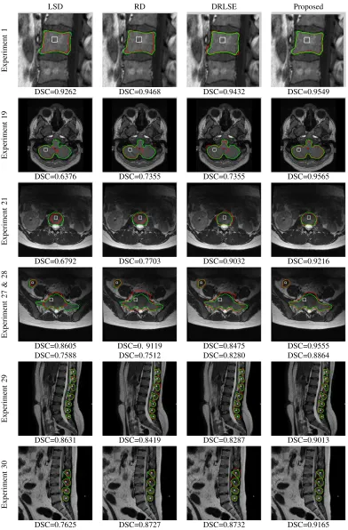
The second set of experiments evaluates the proposed method on real medical images and compares it with LSD, RD and DRLSE. This experiment is divided in two parts. In Part 1, the number of iterations for all evaluated methods is set to the number required to achieve convergence by our method. In Part 2, we increase the number of iterations used in Part 1 in order to evaluate the accuracy of LSD, RD and DRLSE as the number of iterations in Part 1 increases. Table II tabulates the DSC values for different regions of MRI and CT slices. Experiments 1-15 represent different regions of different MRI slices of a spinal cord (vertebral body, sagittal view), Experiments 16 represents a region of an MRI slice of a brain (the caudate nucleus is the object to be segmented), Experiments 17 and 18 represent two regions of an MRI slice of a pelvis; Experiments 19 and 20 represent two regions of a CT slice of a skull, Experiments 21-28 represent different regions of MRI slices of lumbar discs, and Experiments 29-30 represent different regions of two different MRI slices of a spinal cord (spinous process, sagittal view). Experiments 21-28 represent very challenging cases where the target regions have intensities very similar to those of the surrounding regions, thus making it difficult to clearly delineate the objects’ boundaries.

(8)

JOURNAL OF LA_{TEX CLASS FILES} ₇

LSD RD DRLSE Proposed

Experiment

1

DSC=0.9262 DSC=0.9468 DSC=0.9432 DSC=0.9549

Experiment

19

DSC=0.6376 DSC=0.7355 DSC=0.7355 DSC=0.9565

Experiment

21

DSC=0.6792 DSC=0.7703 DSC=0.9032 DSC=0.9216

Experiment

27

&

28

DSC=0.8605 DSC=0. 9119 DSC=0.8475 DSC=0.9555 DSC=0.7588 DSC=0.7512 DSC=0.8280 DSC=0.8864

Experiment

29

DSC=0.8631 DSC=0.8419 DSC=0.8287 DSC=0.9013

Experiment

30

[image:8.612.112.504.91.687.2]

DSC=0.7625 DSC=0.8727 DSC=0.8732 DSC=0.9165

(9)

JOURNAL OF LA_{TEX CLASS FILES} ₈

LSD RD DRLSE Proposed

Experiment

1

DSC=0.7246 DSC=0.9203 DSC=0.08439 DSC=0.09551

Experiment

19

DSC=0.6844 DSC=0.7267 DSC=0.9480 DSC=0.9648

Experiment

21

DSC=0.8420 DSC=0.8968 DSC=0.8314 DSC=0.9183

Experiment

27

&

28

DSC=0.9009 DSC=0.8400 DSC=0.7280 DSC=0.9545 DSC=0.7714 DSC=0.6939 DSC=0.8345 DSC=0.8844

Experiment

29

DSC=0.8148 DSC=0.7332 DSC=0.7557 DSC=0.9135

Experiment

30

[image:9.612.112.504.91.686.2]

DSC=0.8919 DSC=0.8739 DSC=0.8219 DSC=0.9209

(10)

JOURNAL OF LA_{TEX CLASS FILES} ₉

TABLE II

SEGMENTATION ACCURACY OF VARIOUS LEVEL SET METHODS FOR REAL MEDICAL IMAGES.

Exp. DSCPart 1 No. Part 2

iterations DSC iterationsNo. LSD RD DRLSE Proposed approach LSD RD DRLSE Proposed approach

1 0.9262 0.9468 0.9432 0.9549 50 0.7246 0.9203 0.8438 0.9551 80 2 0.9370 0.9437 0.9016 0.9315 50 0.7868 0.5297 0.8913 0.9247 100 3 0.9451 0.9679 0.9501 0.9686 50 0.6873 0.5651 0.6082 0.9686 100 4 0.9391 0.9560 0.9311 0.9595 50 0.7638 0.8676 0.8741 0.9590 60 5 0.9368 0.9603 0.9552 0.9636 50 0.5563 0.9277 0.9544 0.9617 100 6 0.8814 0.9254 0.9166 0.9340 50 0.7695 0.8940 0.8205 0.9352 100 7 0.9085 0.9330 0.9412 0.9589 50 0.7233 0.4730 0.9397 0.9582 100 8 0.9417 0.8375 0.9165 0.9543 50 0.7041 0.8200 0.7235 0.9538 100 9 0.8128 0.8234 0.9445 0.9472 50 0.9364 0.9422 0.9461 0.9479 100 10 0.9070 0.8745 0.9332 0.9468 50 0.8609 0.9067 0.9335 0.9468 100 11 0.8821 0.8944 0.9420 0.9484 50 0.9218 0.9541 0.9434 0.9487 100 12 0.7934 0.8006 0.8123 0.9565 50 0.9055 0.8176 0.8152 0.9569 100 13 0.7150 0.7081 0.9526 0.9674 50 0.7392 0.9560 0.9252 0.9538 100 14 0.8875 0.9058 0.9463 0.9443 50 0.9015 0.9437 0.9466 0.9500 100 15 0.8496 0.7589 0.9577 0.9444 50 0.9466 0.9527 0.9571 0.9482 100 16 0.9584 0.7747 0.9764 0.9670 50 0.7848 0.9507 0.9776 0.9791 100 17 0.9397 0.7643 0.9641 0.9516 50 0.6591 0.9294 0.9767 0.9727 100 18 0.8643 0.8794 0.8510 0.9157 50 0.8076 0.8379 0.8510 0.9157 100 19 0.6376 0.6416 0.7355 0.9565 100 0.6844 0.7267 0.9480 0.9648 140 20 0.7095 0.7388 0.9273 0.9632 100 0.7971 0.8418 0.8680 0.9632 140 21 0.6792 0.7703 0.8874 0.9216 60 0.7812 0.8837 0.8314 0.9183 80 22 0.8504 0.8371 0.9032 0.9290 60 0.8603 0.8581 0.8877 0.9270 80 23 0.6527 0.7080 0.9182 0.9389 60 0.7004 0.8524 0.8968 0.9372 80 24 0.9057 0.8907 0.8920 0.9406 60 0.8852 0.8697 0.8816 0.9361 80 25 0.5701 0.6172 0.8365 0.9385 60 0.6122 0.6472 0.9099 0.9319 80 26 0.6824 0.7349 0.8174 0.9598 70 0.7014 0.8119 0.8331 0.9462 90 27 0.8605 0.9119 0.8475 0.9555 50 0.9009 0.8400 0.7280 0.9545 80 28 0.7588 0.7512 0.8280 0.8864 100 0.7714 0.6939 0.8345 0.8844 130 29 0.8631 0.8419 0.8287 0.9013 60 0.8148 0.7332 0.7557 0.9135 100 30 0.7625 0.8727 0.8732 0.9165 60 0.8919 0.8739 0.8219 0.9209 100

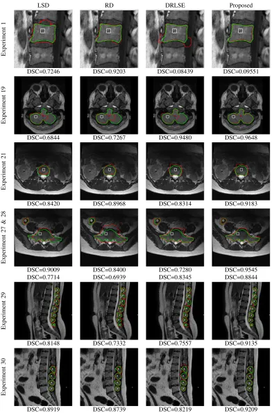
tend to result in leakage as the number of iteration increases; see for example Experiments 2, 3 and 4, Part 2. For the challenging cases (Experiments 21-28), our method achieves convergence before the other evaluated methods and results in higher DSC values. For Experiments 29-30, the regions we intend to delineate are delimited by weak edges. LSD, RD and DRLSE do not converge in the tabulated number of iterations in Part 1 and consequently, tend to result in significant leakage as the number of iteration increases in Part 2. The DSC values attained for these experiments show that the proposed method is also capable to outperform the other methods for these images.

It is important to mention that leakage in DRLSE may be the result of the distance regularization term and area term forcing the zero level set to continue to evolve when the zero level set is already at the desired boundary. Even though our proposed method also employs the distance regularization employed by DRLSE, it prevents leakage and achieves convergence by

weighting the Length2 andArea2 terms according to local

edge features. This confirms the advantage of our weighting approach.

Visual results for Part 1 experiments are shown in Fig. 7. Note that the images in the depicted experiments contain

several intensity inhomogeneities. The third and fourth rows represent challenging cases where the target objects have intensities very similar to the surrounding regions. It can be seen that our method is capable of detecting regions delineated by weak edges. The other evaluated methods (see Columns 1-3 of Fig. 7), fail to correctly segment the regions for the same number of iterations required by our method. Although RD and DRLSE attain an accuracy similar to that obtained by our method for Experiment 1, these methods fail when they are allowed to iterate further, as shown in Fig. 8. Among the most challenging regions are those in Experiment 27 and 28 (fourth row of Fig. 7). In this case, our method successfully detects the cecum region (Experiment 27). This region is characterized by very weak edges. Note that all methods fail to correctly detect the upper edge of the sacrum region (Experiment 28). However, our method is the one that results in the least amount of leakage and thus, the highest DCS value.

(11)

JOURNAL OF LA_{TEX CLASS FILES} ₁₀

control the influence of various energy terms, can improve segmentation accuracy and minimize leakage.

D. Comparisons to PBLS

(a) (b)

Fig. 9. (a) Synthetic phantom. The three circles in each column, from top to bottom, have a radius of 17, 20, and 23 pixels, respectively. (b) Contours obtained by PBLS (yellow) and our proposed method (red). The white curves denote the initial contours.

(a) (b)

Fig. 10. (a) Ultrasound image of the left ventricle of the heart. (b) Contours obtained by PBLS (yellow) and our proposed method (red). The white curve denotes the initial contour.

The third set of experiments compares our method to PBLS on synthetic images and real ultra sound images. PBLS has been shown to perform very well in the presence of weak edges. PBLS uses a similar alignment term as the one proposed by Kimmel’s method. Fig. 9 and Fig. 10 show visual results attained by PBLS and the proposed method on a synthetic and ultra sound image, respectively. Note that both of these images depict very weak edges and high levels of noise. For the case of PBLS, we use the parameters that provide the best edge map for each image. From Fig. 9, we observe that the contours produced by PBLS tend to cover more area of the synthetic circles than the proposed method. This is due to the phase-based edge indicator used by PBLS to detect the edges. However, the proposed method attains very competitive results in the ultra sound image depicted in Fig. 10. It is interesting to note that our proposed method tends to stop at the very weak edge depicted in the lower right part of the ventricle of Fig. 10,while PBLS tends to stop at the stronger edge. This is expected, as our proposed method averages edge features overkcontours adjacent to the evolving contour, which helps evolving contour to conform to very weak edges.

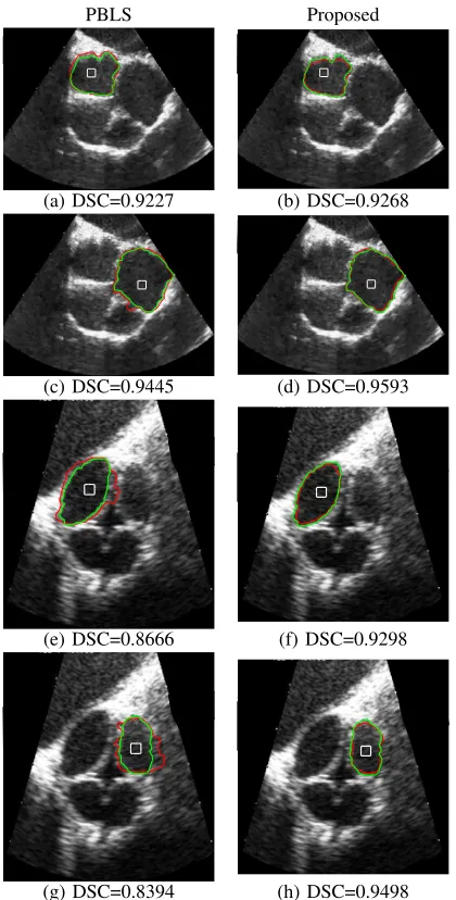
Fig. 11 shows visual results and DSC values attained by PBLS and our proposed method in more challenging ultra-sound images. Note that our method attains very competitive

results for the regions of Fig. 11 (a)-(d), while it outperforms PBLS for the regions of Fig. 11 (e)-(h).

PBLS Proposed

(a) DSC=0.9227 (b) DSC=0.9268

(c) DSC=0.9445 (d) DSC=0.9593

(e) DSC=0.8666 (f) DSC=0.9298

[image:11.612.335.545.89.503.2]

(g) DSC=0.8394 (h) DSC=0.9498

Fig. 11. Visual results and DSC values attained by PBLS and the proposed method in ultra sound images of the heart. Each row corresponds to a region. The white curves denote the initial contours, the red curves represent the final contour and the green curves represent the ground truth.

E. Comparisons to region-based active contours

The fourth set of experiments compares our method to Kimmel’s method on synthetic images and real medical im-ages. Let us recall that Kimmel’s method is a region-based method. It is important to mention that region-based methods are usually based on the Mumford-Shah functional [56]. For example, the method of active contours without edges (Chan-Vese model) solves the piecewise constant Mumford-Shah model but restricts the solution to be a piecewise constant solution with only two constants [6]. Other proposals have successfully solved the energy minimization problem proposed by Mumford and Shah by convex optimization, such as those by Cai, Chan et al.[57], [58].

[image:11.612.52.295.112.236.2] [image:11.612.53.295.299.421.2]

(12)

JOURNAL OF LA_{TEX CLASS FILES} ₁₁

(a) DSC=0.9629 (b) DSC=0.5780 (c) DSC=0.6392 (d) DSC=0.0001

[image:12.612.53.299.66.207.2]

(e) DSC=0.9530 (f) DSC=0.9746 (g) DSC=0.8954 (h) DSC=0.9305

Fig. 12. Visual results and DSC values for synthetic images (columns 1 and 2) and real medical images (columns 3 and 4). The first row corresponds to Kimmel’s method, while the second row corresponds to our method. Column 3 depicts a X-ray vessel image, and column 4 depicts an MRI slice of an abdominal axial cross sectional view of the human body. The white curves denote the initial contours, the red curves represent the final contour and the green curves represent the ground truth.

show that Kimmel’s method outperforms ours for the synthetic image in Fig. 12 (a). This is mainly due to the fact that Kimmel’s method incorporates a region-based force into the model, which increases accuracy when two regions can be easily detected in the image. Our method, however, attains a very similar DSC value to that attained by Kimmel’s in this image. For cases where no two regions can be easily detected, Kimmel’s method is outperformed by ours. This is evidenced in the synthetic image in Fig. 12 (b), where it is difficult to delineate two regions due to the weak edges and the intensity inhomogeneities. Similar results are obtained for the real medical images in Fig. 12 (c) and (d). Our method achieves higher DCS values for these images. It is interesting to note the performance of Kimmel’s method on the image in Fig. 12 (d). As mentioned before, this method attempts to detect two homogeneous regions. Therefore, the detected two regions in this case correspond to those that appear to be the most similar regions in terms of intensities.

F. Sensitivity to position of initial contour

The last set of experiments evaluates the sensitivity to the initial contour’s position of the edge-based methods tabulated in Table II. To this end, we employ different positions for the initial contour on synthetic images and real medical images. Visual results and DSC values are shown in Fig. 13 and 14. All methods have been evaluated with the same number of iterations. In Fig. 13, we show results for a noisy synthetic image. In this case, we tested the case of initializing the contour inside and outside the target regions. These results show that our method successfully detects the objects’ boundary even when the position of the initial contour is located outside the target regions. Our method also achieves the highest DSC values. Fig. 14 demonstrates the robustness of the proposed method with different initial contours on a real medical image. In this case, RD performs better than LSD and DRLSE, as it is capable to conform to most of the desired

boundary regardless of the position of the initial contour. LSD particularly fails when the initial contour is located close to a weak boundary. Our method successfully conforms to the desired boundary with high accuracy for all initialization positions. It is interesting to see that the proposed method results in very similar DSC values for this medical image regardless the position of the initial contour. This confirms

the effectiveness of weight ω in our method to control the

influence of forces according to local features.

LSD RD DRLSE Proposed method

[image:12.612.314.564.182.335.2]

Fig. 13. Segmentation results on a synthetic image after 100 iterations using different positions for the initial contour. The white curves denote the initial contours, the red curves represent the final contour and the green curves represent the ground truth. Each row shows results for a different initial position.

LSD RD DRLSE Proposed method

(i) DSC=0.7199 (j) DSC=0.7670 (k) DSC=0.8791 (l) DSC=0.9565

Fig. 14. Segmentation results on a MRI slice of a spinal cord (vertebral body, sagittal view) after 50 iterations using different positions for the initial contour. The white curves denote the initial contours, the red curves represent the final contour and the green curves represent the ground truth. Each row shows results for a different initial position.

G. Computational complexity

[image:12.612.312.564.403.637.2]