Improving the accuracy of likelihood based inference in meta analysis and meta regression

(1)

Original citation:

Kosmidis, Ioannis, Guolo, A. and Varin, C.. (2017) Improving the accuracy of likelihood-based inference in meta-analysis and meta-regression. Biometrika, 104 (2). pp. 489-496.

Permanent WRAP URL:

http://wrap.warwick.ac.uk/98834

Copyright and reuse:

The Warwick Research Archive Portal (WRAP) makes this work by researchers of the University of Warwick available open access under the following conditions. Copyright © and all moral rights to the version of the paper presented here belong to the individual author(s) and/or other copyright owners. To the extent reasonable and practicable the material made available in WRAP has been checked for eligibility before being made available.

Copies of full items can be used for personal research or study, educational, or not-for profit purposes without prior permission or charge. Provided that the authors, title and full bibliographic details are credited, a hyperlink and/or URL is given for the original metadata page and the content is not changed in any way.

Publisher’s statement:

This is a pre-copyedited, author-produced version of an article accepted for publication in Biometrika following peer review. The version of record I. Kosmidis, A. Guolo, C. Varin; Improving the accuracy of likelihood-based inference in meta-analysis and meta-regression, Biometrika, Volume 104, Issue 2, 1 June 2017, Pages 489–496,

https://doi.org/10.1093/biomet/asx001 is available online at: https://doi.org/10.1093/biomet/asx001

A note on versions:

The version presented here may differ from the published version or, version of record, if you wish to cite this item you are advised to consult the publisher’s version. Please see the ‘permanent WRAP url’ above for details on accessing the published version and note that access may require a subscription.

(2)

Improving the accuracy of likelihood-based inference in

meta-analysis and meta-regression

I. Kosmidis

Department of Statistical Science University College London London, WC1E 6BT, U.K

[email protected]

A. Guolo

Department of Statistical Sciences University of Padova

Via Cesare Battisti, 241, 35121 Padova, Italy [email protected]

C. Varin

Department of Environmental Sciences, Informatics and Statistics, Ca’ Foscari University of Venice

Via Torino 150, 30170 Venezia Mestre, Italy [email protected]

May 24, 2017

Abstract

Random-effects models are frequently used to synthesise information from different stud-ies in meta-analysis. While likelihood-based inference is attractive both in terms of limiting properties and of implementation, its application in random-effects meta-analysis may result in misleading conclusions, especially when the number of studies is small to moderate. The current paper shows how methodology that reduces the asymptotic bias of the maximum like-lihood estimator of the variance component can also substantially improve inference about the mean effect size. The results are derived for the more general framework of random-effects meta-regression, which allows the mean effect size to vary with study-specific covariates. Keywords: Bias reduction; Heterogeneity; Meta-analysis; Penalized likelihood; Random ef-fect; Restricted maximum likelihood

1 Introduction

Meta-analysis is a widely applicable approach to combining information from different studies about a common effect of interest. A popular framework for accounting for the heterogeneity between studies is the random-effects specification in DerSimonian & Laird (1986). There is ample evidence that frequentist inference for this specification can result in misleading conclu-sions, especially if inference is carried out by relying on first-order asymptotic arguments in the common setting of small or moderate number of studies (e.g., van Houwelingen et al., 2002; Guolo & Varin, 2015). The same considerations apply to the random-effects meta-regression model, which is a direct extension of random-effects meta-analysis allowing for study-specific

(3)

covariates. Proposals presented to account for the finite number of studies include modification of the limiting distribution of test statistics (Knapp & Hartung, 2003), restricted maximum like-lihood (Viechtbauer, 2005) and second-order asymptotics (Guolo, 2012). Recently, Zeng & Lin (2015) suggested a double resampling approach that outperforms several alternatives in terms of empirical coverage probability of confidence intervals for the mean effect size.

The current paper studies the extent of the bias of the maximum likelihood estimator of the random-effect variance and introduces a bias-reducing penalized likelihood that yields a substantial improvement in the estimation of the random-effect variance. The bias-reducing penalized likelihood is related to the approximate conditional likelihood of Cox & Reid (1987) and the restricted maximum likelihood for inference about the random-effects variance. The order of the penalty function allows the derivation of a χ2 approximation of the distribution of the logarithm of the penalized likelihood ratio statistic, which can be used for inference about the fixed-effect parameters. Real-data examples and two simulation studies illustrate the improvement in finite-sample performance against alternatives from the recent literature.

2 Random-effects meta-regression and meta-analysis

Suppose there are K studies about a common effect of interest, each of them providing pairs of summary measures (yi,σˆi2), where yi is the study-specific estimate of the effect, and ˆσi2 is the associated estimation variance (i= 1, . . . , K). In some situations, the pairs (yi,σˆ2_i) may be accompanied by study-specific covariates xi = (xi1, . . . , xip)>, which describe the heterogeneity

across studies. In the meta-analysis literature, it is usually assumed that the within-study vari-ances ˆσ_i2 are estimated well enough to be considered as known and equal to the values reported in each study. Under this assumption, the random-effects meta-regression model postulates that y1, . . . , yK are realizations of random variables Y1, . . . , YK, respectively, which are independent conditionally on independent random effects U1, . . . , UK, and the conditional distribution of Yi

given Ui = ui is N(ui +x_i>β,ˆσ2_i), where β is an unknown p-vector of effects. The random effect Ui is typically assumed to be distributed according toN(0, ψ), whereψ accounts for the between-study heterogeneity.

In matrix notation, and conditionally on (U1, . . . , UK)> = u, the random-effects

meta-regression model is

Y =Xβ+u+, (1)

whereY = (Y1, . . . , YK)>,X is the model matrix of dimensionK×pwithx>i in itsith row, and = (1, . . . , K)>is a vector of independent errors each with aN(0,σˆi2) distribution. Under this specification, the marginal distribution ofY is multivariate normal with mean Xβ and variance

ˆ

Σ +ψIK, where IK is theK×K identity matrix and ˆΣ = diag(ˆσ21, . . . ,σˆK2). The random-effects meta-analysis model is a meta-regression model where X is a column of ones.

The random-effects meta-regression model is used here as a working model for theoretical development. In light of the recent criticisms of the assumption of known within-study variances (see, for example Hoaglin, 2015),§4 and the Supplementary Material illustrate the good perfor-mance of the derived procedures under more realistic scenarios, where the estimation variances are directly related to the estimates of the summary measure.

The parameter β is naturally estimated by weighted least squares as

ˆ

β(ψ) ={X>W(ψ)X}−1X>W(ψ)Y , (2)

with W(ψ) = ( ˆΣ +ψIK)−1. Then, inference about β can be based on the fact that under model (1), ˆβ(ψ) has an asymptotic normal distribution with meanβand variance

(4)

In this case, the reliability of the associated inferential procedures critically depends on the avail-ability of an accurate estimate of the between-study varianceψ. A popular choice is the DerSimo-nian & Laird (1986) estimator ˆψDL= max{0,(Q−n+p)/A}, whereQ= (Y −XβˆF)>Σˆ−1(Y −

XβˆF) is the Cochran statistic, with ˆβF = ˆβ(0) and A= tr( ˆΣ−1)−tr{(X>Σˆ−1X)−1X>Σˆ−2X}.

Viechtbauer (2005) presents evidence of the loss of efficiency of ˆψDL, which can impact inference;

3 Bias reduction

3.1 Bias-reducing penalized likelihood

From the results in Kosmidis & Firth (2009, 2010), the first term in the expansion of the bias function of the maximum likelihood estimator is found to be b(θ) ={0_p>, bψ(ψ)}>, where

bψ(ψ) =−

tr{W(ψ)H(ψ)}

tr{W(ψ)2_} , (5)

withH(ψ) =X{X>W(ψ)X}−1_X>_W₍_ψ_{). A sketch derivation for (5) is given in the Appendix.}

In what followsb(θ) is called the first-order bias.

The non-zero entries ofW(ψ) and the diagonal entries of H(ψ) are all necessarily positive, so the maximum likelihood estimator of ψ is subject to downward bias, which, as also noted in Viechtbauer (2005), affects inference aboutβ, by over-estimating the non-zero entries ofW(ψ), and hence over-estimating the information matrix

F(θ) =−Eθ

∂2`(θ) ∂θ∂θ>

=

X>W(ψ)X 0p 0>_p 1₂trW(ψ)2

. (6)

This over-estimation ofF(θ) can result in hypothesis tests with large Type I error and confidence intervals or regions with actual coverage appreciably lower than the nominal level.

An estimator that corrects for the first-order bias of ˆθML results from solving the adjusted

score equations s∗(θ) =s(θ)−F(θ)b(θ) = 0p+1 (Firth, 1993; Kosmidis & Firth, 2009).

Substi-tuting (4), (5) and (6) in the expression for s∗(θ) gives that the adjusted score functions forβ and ψ ares∗_β(θ) =sβ(θ) and

(5)

respectively. The expression for the differential of the log-determinant can be used to show that s∗_β(θ) and s∗_ψ(θ) are the derivatives of the penalized log-likelihood function

`∗(θ) =`(θ)−1

2log

F₍_ββ₎(ψ)

, (8)

where `(θ) is as in (3), F₍_ββ₎(ψ) = X>W(ψ)X is the β-block of the information matrix F(θ), and |·| denotes determinant, so the solution of the adjusted score equations is the maximum penalized likelihood estimator ˆθMPL.

Forβ = ˆβ(ψ), expression (8) reduces to both the logarithm of the approximate conditional likelihood of Cox & Reid (1987) for inference about ψ, when β is treated as a nuisance com-ponent, and to the restricted log-likelihood function of Harville (1977). Hence, maximising the bias-reducing penalized log-likelihood (8) is equivalent to calculating the maximum restricted likelihood estimator forψ. The latter estimator was originally constructed to reduce underesti-mation of variance components in finite samples as a consequence of failing to account for the degrees of freedom that are involved in the estimation of the fixed effects β. Smyth & Verbyla (1996) and Stern & Welsh (2000) have shown the equivalence of the restricted log-likelihood with approximate conditional likelihood in the more general context of inference about variance components in normal linear mixed models.

3.2 Estimation

Given a starting value ψ(0) for ψ, the following iterative process has a stationary point that maximizes (8). At thejth iteration (j= 1,2, . . .), a new candidate valueβ(j+1)forβis obtained as the weighted least squares estimator (2) at ψ = ψ(j)_{; a candidate value for} _ψ(j+1) _{is then}

computed by a line search for solving the adjusted score equation (7) evaluated at β =β(j+1). The iteration is repeated until either the candidate values do not change across iterations or the adjusted score functions are sufficiently close to zero.

3.3 Penalized likelihood inference

The profile penalized likelihood function can be used to construct confidence intervals and re-gions, and carry out hypothesis tests for β. If β = (γ>, λ>)>, and ˆλMPL,γ and ˆψMPL,γ are the estimators of λ and ψ, respectively, from maximising (8) for fixed γ, then the logarithm of the penalized likelihood ratio statistic 2{`∗(ˆγMPL,ˆλMPL,ψˆMPL)−`∗(γ,ˆλMPL,γ,ψˆMPL,γ)}has the usual limiting χ2

q distribution, where q = dim(γ). To derive this limiting result, note that the adjustment to the scores in (4) is additive and O(1), so the extra terms depending on it and its derivatives in the asymptotic expansion of the penalized likelihood disappear as information increases.

The impact of using the penalized likelihood for estimation and inference in random-effects meta-analysis and meta-regression is more profound for a small to moderate number of studies. As the number of studies increases, the log-likelihood derivatives dominate the bias-reducing adjustment in (7) in terms of asymptotic order. As a result, inference based on the penalized likelihood becomes indistinguishable from likelihood inference.

(6)

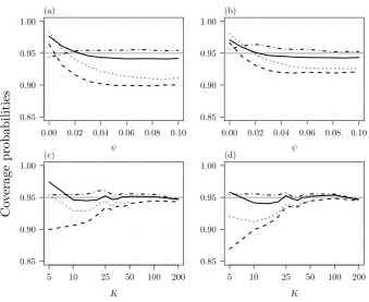
0.00 0.02 0.04 0.06 0.08 0.10 0.85

0.90 0.95 1.00

ψ (a)

0.00 0.02 0.04 0.06 0.08 0.10 0.85

0.90 0.95 1.00

ψ (b)

0.85 0.90 0.95 1.00

K

(c)

5 10 25 50 100 200

0.85 0.90 0.95 1.00

K

(d)

5 10 25 50 100 200

Co

[image:6.595.121.461.84.361.2]

verage probabilities

Figure 1: Empirical coverage probabilities of two-sided confidence intervals for β for increasing ψ, when (a) K = 10 and (b) K = 20, and for increasing K (in log scale) when (c) ψ = 0.03 and (d) ψ= 0.07. The curves correspond to profile penalized likelihood (solid), DerSimonian & Laird method (dashed), Zeng & Lin double resampling (dotted; available only forK ≤50), and Skovgaard’s statistic (dotted-dashed). The grey horizontal line is the target 95% nominal level.

4 Simulation studies

4.1 Random-effects meta-analysis

The simulation studies under the random-effects meta-analysis model (1) are performed using the design in Brockwell & Gordon (2001). Specifically, the study-specific effectsyiare simulated from the random-effect meta-analysis with true effect β = 0.5 and variance ˆσ_i2+ψ, where ˆσ_i2 are independently generated from a χ2₁ distribution multiplied by 0.25 and then restricted to the interval (0.009,0.6). The between-study variance ψ ranges from 0 to 0.1 and the number of studies K from 5 to 200. For each combination of ψ and K considered, 10 000 data sets are simulated using the same initial state for the random number generator.

Zeng & Lin (2015, Section 5) show that their double resampling approach outperforms several existing methods in terms of the empirical coverage probabilities of confidence intervals for β at nominal level 95%. The methods considered in Zeng & Lin (2015) include profile likelihood (Hardy & Thompson, 1996), modified DerSimonian & Laird (see Sidik & Jonkman, 2002; Knapp & Hartung, 2003; Copas, 2003), quantile approximation (Jackson & Bowden, 2009) and the approach described in Henmi & Copas (2010). The present simulation study takes advantage of these previous simulation results, and Figure 1 compares the performance of double resampling with that of the profile penalized likelihood. In order to avoid long computing times, empirical coverage for double-resampling has been calculated only for K ≤50.

(7)

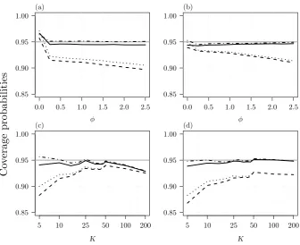
0.0 0.5 1.0 1.5 2.0 2.5 0.85

0.90 0.95 1.00

φ (a)

0.0 0.5 1.0 1.5 2.0 2.5 0.85

0.90 0.95 1.00

φ (b)

0.85 0.90 0.95 1.00

K

(c)

5 10 25 50 100 200 0.85 0.90 0.95 1.00

K

(d)

5 10 25 50 100 200

Co

[image:7.595.122.459.86.360.2]

verage probabilities

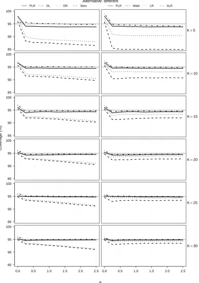
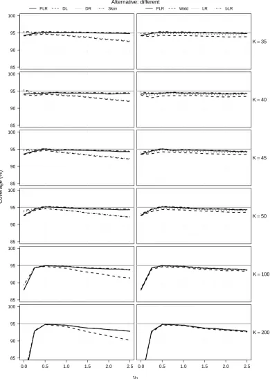
Figure 2: Empirical coverage probabilities of two-sided confidence intervals for δ for increasing φ, when (a) K = 10 and (b) K = 35, and for increasing K (in log scale) when (c) φ = 0.25 and (d) φ = 2. The curves correspond to profile penalized likelihood (solid), DerSimonian & Laird method (dashed), Zeng & Lin double resampling (dotted), and Skovgaard’s statistic (dotted-dashed). The grey horizontal line is the target 95% nominal level.

Figure 1 also includes results for two alternative confidence intervals. The first uses the classical DerSimonian & Laird estimator ˆβ(ψDL) and its estimated variance 1/PK_i₌₁1/(ˆσi+ ˆψDL).

Not surprisingly, the empirical coverage of this confidence interval is grossly smaller than the nominal confidence level. The second interval is used for reference and results from the numerical inversion of Skovgaard’s statistic, which is designed to produce second-order accurate p-values for tests on the mean effect size (Guolo, 2012; Guolo & Varin, 2012). The profile penalized likelihood interval has comparable performance to that based on Skovgaard’s statistic, with the latter having empirical coverage slightly closer to the nominal level for a wider range of values for ψ. In general, though, the numerical inversion of Skovgaard’s statistic can be unstable due to the discontinuity of the statistic around the maximum likelihood estimator. In contrast, the calculation of profile penalized likelihood intervals is not prone to such instabilities. The penalized likelihood also results in a bias-reduced estimator of ψ, whose reliable estimation is often of interest in medical studies (Veroniki et al., 2016).

4.2 Standardized mean differences from two-arm studies

(8)

are calculated by simulating individual-within-study data. Specifically, we assume that the ith study consists of two arms withniindividuals each, and thatn1, . . . , nK are independent uniform draws from the integers {30,31, . . . ,100}. Then, conditionally on a random effectαi ∼N(0, φ), we assume that the observation zi,rj for the jth individual in the rth arm is the realisation of a N(µ+Ir(δ+αi)σ, σ2) random variable, where I1 = 0 and I2 = 1. The difference between

the marginal variances of the arms increases with φ. The true effects are set to µ = 0, σ = 1 and δ = −2. The study-specific effect of interest is δ, estimated using the standardized mean difference yi = Ji(¯zi,2−zi,¯ 1)/si, where s2_i is the pooled variance from the two arms of the ith

study, and Ji = 1−3/{8(ni −1)−1} is the Hedges correction (see, e.g., Borenstein, 2009, Chapter 4). The corresponding estimated variance for yi is ˆσ_i2 = 2Ji/ni+Jiy_i2/(4ni), which is a quadratic function of yi. The between-study varianceφranges from 0 to 2.5 and the number of studies K from 5 to 200. For each combination of φand K considered, 10 000 data sets are simulated using the same initial state for the random number generator.

Figure 2 shows the empirical coverage of the confidence intervals forδbased on the methods that were examined in Figure 1. Empirical coverage for double-resampling has again been calculated only for K ≤ 50. The good performance of the profile penalized likelihood interval and the interval based on the Skovgaard’s statistic persists for small and moderate number of studies, even under the alternative data generating process. The performance of the intervals based on the DerSimonian & Laird estimator and double resampling is, again, poor.

Figure 2 also illustrates the effect of increasing the number of studies under the alternative specification of the data generating process. As the number of studies increases, the inadequacy of the assumptions of the working random-effects meta-regression model becomes more notable. Model mis-specification will eventually result in loss of coverage for all methods examined here, including the intervals based on profile penalized likelihood and the Skovgaard’s statistic.

The Supplementary Material provides the full results from this study and two other simula-tion studies, where the summary measures are log-odds-ratios from a case-control study.

5 Case study: meat consumption data

Larsson & Orsini (2014) investigate the association between meat consumption and relative risk of all-cause mortality. The data include 16 prospective studies, eight of which are about unprocessed red meat consumption and eight about processed meat consumption. We consider meta-regression with a covariate taking value 1 for processed red mean and 0 for unprocessed. The DerSimonian & Laird estimate ofψis ˆψDL= 0.57×10−2, the maximum likelihood estimate is

ˆ

ψML= 0.85×10−2 and the maximum penalized likelihood estimate is the largest with ˆψMPL =

1.18×10−2. The estimates of β are ˆβML = (0.10,0.11)>, ˆβMPL = (0.09,0.11)> and ˆβDL =

(0.11,0.10)>, where the first element in each vector corresponds to the intercept and the second to meat consumption.

The DerSimonian & Laird method indicates some evidence for a higher risk associated to the consumption of red processed meat with a p-value of 0.027. In contrast, the penalized likelihood ratio and Skovgaard’s statistic suggest that there is rather weak evidence for higher risk, with p-values of 0.066 and 0.073, respectively.

The Supplementary Material contains a simulation study under the maximum likelihood fit that illustrates that the maximum likelihood estimator of ψ is negatively biased. The other estimators almost fully compensate for that bias, but ˆψMPL is appreciably more efficient than

ˆ

ψDL. The simulation study therein is also used to illustrate the good performance of the penalized

(9)

6 Supplementary material

The Supplementary Material provides R (R Core Team, 2016) code to reproduce the case study in § 5, and another analysis. The full results of the simulations are provided including the performance of confidence intervals based on alternative methods.

Acknowledgements

This work was partially supported by grants ‘IRIDE’, Ca’ Foscari University of Venice and ‘Progetti di Ricerca di Ateneo 2015’, University of Padova. The authors thank David Firth for discussions and feedback on an early version of the paper. The authors are also grateful to two anonymous Referees, the Associate Editor and the Editor, for helpful comments and suggestions, and thankful to Sophia Kyriakou for bringing to their attention some inconsequential typos that have been fixed in the current version. In particular, expression (3) has `(θ) = 1₂...instead of `(θ) = −1₂..., and the middle expressions in the equations for sψ(θ) and s∗ψ(θ) in (4) and (7), respectively, have been multiplied by a factor of 1/2.

Appendix A: derivation of the expression for the first-order bias

The first-order bias of ˆθ₍_{M L}₎ has the form b(θ) = − {F(θ)}−1A(θ) (Kosmidis & Firth, 2010), where A(θ) has components

At(θ) =− 1 2tr

h

{F(θ)}−1{Pt(θ) +Qt(θ)}

i

(t= 1, . . . , p+ 1).

There, Pt(θ) =Eθ{s(θ)s(θ)>st(θ)}and Qt(θ) =Eθ{−I(θ)st(θ)}.

The model assumptions imply that Eθ{Ri(β)m} is 0 if m is odd and (m−1)!!/wi(ψ)m/2 if m is even, where wi(ψ) = 1/(ˆσ2i +ψ), and (m−1)!! denotes the double factorial of m−1 (m= 1,2, . . .;i= 1, . . . , K). Direct matrix calculations give

Pt(θ) +Qt(θ) = 0(p+1)×(p+1) (t= 1, . . . , p) ; Pp+1(θ) +Qp+1(θ) =

X>W(ψ)2X 0p 0>_p 0

,

where 0p×p is thep×pzero matrix. So, At(θ) = 0 for t∈ {1, . . . , p}and

Ap+1(θ) = tr

n

X>W(ψ)Xo−1X>W(ψ)2X

= tr{W(ψ)H(ψ)} .

Inserting the expressions for the components of A(θ) into the expression for b(θ) gives b(θ) =

{0>_p, bψ(ψ)}>, wherebψ(ψ) is as in (5).

References

Borenstein, M.,Hedges, L. V.,Higgins, J. P. T.&Rothstein, H. R.(2009).

Introduc-tion to Meta-Analysis. Chichester, West Sussex: Wiley.

Brockwell, S. E. &Gordon, I. N. (2001). A comparison of statistical methods for

meta-analysis. Stat. Med.20, 825–40.

Copas, J.(2003) Letters to the editor: a simple confidence interval for meta-analysis. Sidik K.,

(10)

Cox, D. R.&Reid, N.(1987). Parameter orthogonality and approximate conditional inference

(with discussion). J. R. Statist. Soc. B 49, 1–39.

DerSimonian, R. & Laird, N. (1986). Meta-analysis in clinical trials. Control. Clin. Trials

7, 177–88.

Firth, D. (1993). Bias reduction of maximum likelihood estimates. Biometrika 80, 27–38.

Guolo, A. (2012). Higher-order likelihood inference in meta-analysis and meta-regression.

Stat. Med.31, 313–27.

Guolo, A. & Varin, C. (2012). The R package metaLik for likelihood inference in

meta-analysis. J. Stat. Softw.50, 1–14.

Guolo, A.&Varin, C.(2015). Random-effects meta-analysis: The number of studies matters.

Stat. Methods Med. Res., to appear.

Hardy, R. J.&Thompson, S. G.(1996). A likelihood approach to meta-analysis with random

effects. Stat. Med.15, 619–29.

Harville, D. A. (1977). Maximum likelihood approaches to variance component estimation

and to related problems. J. Amer. Stat. Ass.72, 320–38.

Henmi, M. &Copas, J. B. (2010). Confidence intervals for random effects meta-analysis and

robustness to publication bias. Stat. Med.29, 2969–83.

Hoaglin, D. C. (2015). We know less than we should about methods of meta-analysis.

Res. Syn. Meth. 6, 287–9.

van Houwelingen, H. C., Arends, L. R. & Stijnen, T. (2002). Advanced methods in

meta-analysis: multivariate approach and meta-regression. Stat. Med.21, 589–624.

Jackson, D. & Bowden, J. (2009). A re-evaluation of the ‘quantile approximation method’

for random effects meta-analysis. Stat. Med. 28, 338–48.

Knapp, G. & Hartung, J.(2003). Improved tests for a random effects meta-regression with

a single covariate. Stat. Med. 22, 2693–710.

Kosmidis, I. & Firth, D. (2009). Bias reduction in exponential family nonlinear models.

Biometrika 96, 793–804.

Kosmidis, I. &Firth, D.(2010). A generic algorithm for reducing bias in parametric estima-tion. Electron. J. Stat.4, 1097–112.

Larsson, S. C.&Orsini, N.(2014) Red meat and processed meat consumption and all-cause

mortality: A meta-analysis. Am. J. Epidemiol. 179, 282–89.

R Core Team (2016). R: A Language and Environment for Statistical Computing. Vienna,

Austria: R Foundation for Statistical Computing. http://www.R-project.org.

Smyth, G. K. & Verbyla, A. P. (1996). A conditional likelihood approach to residual

maximum likelihood estimation in generalized linear models. J. R. Statist. Soc. B 58, 565– 72.

Stern, S. E. & Welsh, A. H. (2000). Likelihood inference for small variance components.

(11)

Sidik, K.&Jonkman, J. N.(2002). A simple confidence interval for meta-analysis.Stat. Med.

21, 3153–9.

Veroniki, A. A., Jackson, D., Viechtbauer, W., Bender, R., Bowden, J., Knapp, G., Kuss, O.,Higgins, J. P. T., Langan, D., andSalanti, G. (2016) Methods to estimate the

between-study variance and its uncertainty in meta-analysis. Res. Syn. Meth. 7, 55–79.

Viechtbauer, W. (2005). Bias and efficiency of meta-analytic variance estimators in the

random-effects model. J. Educ. Behav. Stat. 30, 261–93.

(12)

Supplementary material for

Improving the accuracy of likelihood-based inference in

meta-analysis and meta-regression

I. Kosmidis

Department of Statistical Science University College London London, WC1E 6BT, U.K

[email protected]

A. Guolo

Department of Statistical Sciences University of Padova

Via Cesare Battisti, 241/243, 35121 Padova, Italy

[email protected]

C. Varin

Department of Environmental Sciences, Informatics and Statistics, Ca’ Foscari University of Venice

Via Torino 150, 30170 Venezia Mestre, Italy

[email protected]

January 8, 2017

1 R version, package details and other functions

The current report reproduces the real-data analysis and provides the full results of the simu-lation studies described in the paper “Improving the accuracy of likelihood-based inference in meta-analysis and meta-regression” by I. Kosmidis, A. Guolo and C. Varin. The report also enriches the paper with an extra case-study and the results from two extra simulation scenarios. The outputs in the current report have been produced using R version 3.3.0 (R Development Core Team, 2016), and the R packagemetaLik version 0.42.0 (Guolo & Varin, 2012).

The file functionsMPL.R that accompanies the current report (at the time of writing the file is available from _{http://www.ucl.ac.uk/~ucakiko/files/functionsMPL.R}) provides:

• an R function to maximize the penalized likelihood in expression (8) of the paper for general meta-regression settings (see the function BiasFit);

• an R function to perform hypothesis tests for the parameters of a meta-regression model using the profiles of the penalized likelihood as in §3.3 of the paper (see the function lrtestinfunctionsMPL.R);

• an R implementation of the double resampling approach in Zeng & Lin (2015) for hypoth-esis testing in meta-analysis; and

(13)

2

The following chunk of code loads the required packages and the functions infunctionsMPL.R:

library(metaLik) library(metatest) library(parallel)

## REPLACE THIS WITH LINK TO URL

source(url("http://www.ucl.ac.uk/~ucakiko/files/functionsMPL.R"))

2 Case studies

2.1 Meat consumption data

The data for the analysis in § 5 of the main text is

# Meat consumption data ########################

larsson <- data.frame(logRR = c(-0.3425, 0.2546, 0.1740, 0.1655, -0.0834, 0.0953, 0.2151, 0.3988,

0.0488, 0.1484, 0.2231, 0.2390,

0.1823, 0.3577, 0.0583, 0.1484),

sigma2 = c(0.017224, 0.001271, 0.000663, 0.005027,

0.003383, 0.003603, 0.062186, 0.118504,

0.071613, 0.000310, 0.000501, 0.001160,

0.000759, 0.005087, 0.031266, 0.023078), type = c(rep("non-p", 8), rep("p", 8)))

The variable type is the meat type (p for processed and non-p for non-processed), logRR is the logarithm of the relative risk of all-cause mortality for the highest versus the lowest consumption category, and sigma2is the variance of the logarithm of the relative risk.

The code chunk below fits the random-effects meta-regression model with response logRR, explanatory variable type and summary variances sigma2. The model includes an intercept parameter β1, the parameter β2 for type and the heterogeneity parameter psi. The model

parameters are estimated using maximum likelihood, the DerSimonian & Laird estimator, and maximum penalized likelihood.

m1 <- metaLik(logRR ~ type, data = larsson, sigma2 = sigma2) estimates1 <- BiasFit(m1)

estimates1 <- with(estimates1, data.frame(ML = ML[1:3], DL = DL[1:3], MPL = MPL[1:3])) rownames(estimates1)[3] <- "psi"

round(estimates1, 4)

## ML DL MPL

## (Intercept) 0.0994 0.1060 0.0947 ## typep 0.1064 0.1004 0.1098 ## psi 0.0085 0.0057 0.0118

The following code chunk calculates the p-value for testingβ2 <0 using the DerSimonian &

Laird method, the penalized likelihood ratio and the Skovgaard’s statistic.

pvalue1_dl <- pnorm(m1$DL[2] / sqrt(m1$vcov.DL[2, 2]), lower.tail = FALSE)

pvalue1_pd <- lrtest(m1, what = 2, type = "penloglik", null = 0.0, optMethod = "BFGS", alternative = "greater")$pvalue

pvalue1_Skovgaard <- test.metaLik(m1, param = 2, value = 0, print = FALSE, alternative = "greater")$pvalue.rskov pvalues1 <- c(pvalue1_dl, pvalue1_pd, pvalue1_Skovgaard)

names(pvalues1) <- c("DerSimonian Laird", "Penalized likelihood", "Skovgaard") round(pvalues1, 3)

## DerSimonian Laird Penalized likelihood Skovgaard

(14)

3

The chunk of code below simulates 10 000 independent samples of the 16 logarithms of relative risks under the maximum likelihood fitm1, conditionally ontype andsigma2. For each simulated sample,ψis estimated using maximum likelihood, maximum penalized likelihood and the DerSimonian & Laird estimator. In addition, p-values are computed for the hypothesis

β2 < 0, using the DerSimonian & Laird statistic, the likelihood ratio statistic, the penalized

likelihood ratio statistic and Skovgaard’s statistic.

# Number of cores to be used for the simulations (does /not/ work in Windows machines)

ncores <- 4

nsimu <- 10000

simudata <- simulate(m1, nsim = nsimu, seed = 123) tau2ind <- length(coef(m1)) + 1

typep <- coef(m1)[2]

results <- mclapply(seq.int(ncol(simudata)), function(i) {

mod <- update(m1, data = within(larsson, logRR <- simudata[, i])) out <- BiasFit(mod)

estimates <- data.frame(estimate = with(out, c(ML[tau2ind], DL[tau2ind], MPL[tau2ind])), method = c("ML", "DL", "MPL"))

pvalues <- perform_tests(y = simudata[, i], X = mod$X, sigma2 = mod$sigma2, what = 2, null = typep, B = 1)

pvalues <- data.frame(pvalue = pvalues[c("DL", "LR", "PLR", "Skovgaard"), "pvalues_g"]) pvalues$method <- c("DerSimonian Laird", "Likelihood", "Penalized likelihood", "Skovgaard") list(estimates = estimates, pvalues = pvalues)

[image:14.595.71.529.520.717.2]

}, mc.cores = ncores)

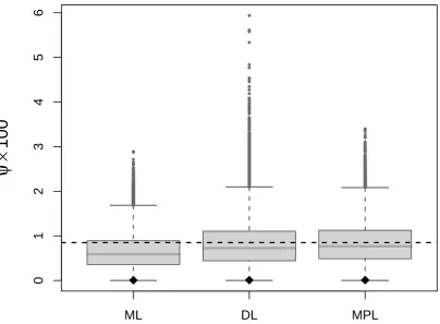
Figure 3 shows boxplots of the estimators ofψcalculated from the 10 000 simulated samples. The dashed lines correspond to the parameters values used for the simulation and the point inside each box is the average of the estimates for the corresponding method. As expected from expression (5) of the main text, the maximum likelihood estimator of ψ is negatively biased, while the other estimators almost fully compensate for that bias. The distribution of the DerSimonian & Laird estimator ofψappears to have a heavier right tail than the maximum penalized likelihood estimator, which links to the findings of past studies on the loss of efficiency of the former (e.g., Viechtbauer, 2005).

The simulated samples are also used below to calculate the empirical p-value distribution (%) for the tests based on the DerSimonian & Laird statistic, the likelihood ratio statistic, the penalized likelihood ratio statistic and Skovgaard’s statistic. The empirical p-value distribu-tion for the penalized likelihood ratio statistic and Skovgaard’s statistic are markedly closer to uniform than for the other methods.

pvalues <- do.call("rbind", lapply(results, function(x) x$pvalues)) pvalues$method <- factor(pvalues$method)

alphas <- c(1.0, 2.5, 5.0, 10.0, 25.0, 50.0, 75.0, 90.0, 95.0, 97.5, 99.0)/100

distr <- with(pvalues, {

sizes <- sapply(alphas, function(alpha) {

tapply(pvalue, method, function(ps) mean(ps < alpha))

})

colnames(sizes) <- format(alphas * 100, digits = 2) round(sizes * 100, 1)

}) distr

## 1.0 2.5 5.0 10.0 25.0 50.0 75.0 90.0 95.0 97.5 99.0 ## DerSimonian Laird 2.5 4.5 7.6 12.4 26.6 49.9 73.4 87.6 92.3 95.2 97.3 ## Likelihood 2.1 4.5 7.6 13.0 27.9 50.1 71.7 86.6 92.2 95.3 97.7 ## Penalized likelihood 1.3 3.0 5.6 11.0 25.9 49.9 73.8 89.0 94.2 96.9 98.6 ## Skovgaard 1.1 2.7 5.0 10.2 25.2 49.9 74.6 89.7 94.9 97.4 98.9

2.2 Local anesthesia data

(15)

4 ● ● ● ● ● ● ● ● ● ● ● ● ● ● ● ● ● ● ● ● ● ● ● ● ● ● ● ● ● ● ● ● ● ● ● ● ● ● ● ● ● ● ● ● ● ● ● ● ● ● ● ● ● ● ● ● ● ● ● ● ● ● ● ● ● ● ● ● ● ● ● ● ● ● ● ● ● ● ● ● ● ● ● ● ● ● ● ● ● ● ● ● ● ● ● ● ● ● ● ● ● ● ● ● ● ● ● ● ● ● ● ● ● ● ● ● ● ● ● ● ● ● ● ● ● ● ● ● ● ● ● ● ● ● ● ● ● ● ● ● ● ● ● ● ● ● ● ● ● ● ● ● ● ● ● ● ● ● ● ● ● ● ● ● ● ● ● ● ● ● ● ● ● ● ● ● ● ● ● ● ● ● ● ● ● ● ● ● ● ● ● ● ● ● ● ● ● ● ● ● ● ● ● ● ● ● ● ● ● ● ● ● ● ● ● ● ● ● ● ● ● ● ● ● ● ● ● ● ● ● ● ● ● ● ● ● ● ● ● ● ● ● ● ● ● ● ● ● ● ● ● ● ● ● ● ● ● ● ● ● ● ● ● ● ● ● ● ● ● ● ● ● ● ● ● ● ● ● ● ● ● ● ● ● ● ● ● ● ● ● ● ● ● ● ● ● ● ● ● ● ● ● ● ● ● ● ● ● ● ● ● ● ● ● ● ● ● ● ● ● ● ● ● ● ● ● ● ● ● ● ● ● ● ● ● ● ● ● ● ● ● ● ● ● ● ● ● ● ● ● ● ● ● ● ● ● ● ● ● ● ● ● ● ● ● ● ● ● ● ● ● ● ● ● ● ● ● ● ● ● ● ● ● ● ● ● ● ● ● ● ● ● ● ● ● ● ● ● ● ● ● ● ● ● ● ● ● ● ● ● ● ● ● ● ● ● ● ● ● ● ● ● ● ● ● ● ● ● ● ● ● ● ● ● ● ● ● ● ● ● ● ● ● ● ● ● ● ● ● ● ● ● ● ● ● ● ● ● ● ● ● ● ● ● ● ● ● ● ● ● ● ● ● ● ● ● ● ● ● ● ● ● ● ● ● ● ● ● ● ● ● ● ● ● ● ● ● ● ● ● ● ● ● ● ● ● ● ● ● ● ● ● ● ● ● ● ● ● ● ● ● ● ● ● ● ● ● ● ● ● ● ● ● ● ● ● ● ● ● ● ● ● ● ● ● ● ● ● ● ● ● ● ● ● ● ● ● ● ● ● ● ● ● ● ● ● ● ● ● ● ● ● ● ● ● ● ● ● ● ● ● ● ● ● ● ● ● ● ● ● ● ● ● ● ● ● ● ● ● ● ● ● ● ● ● ● ● ● ● ● ● ● ● ● ● ● ● ● ● ● ● ● ● ● ● ● ● ● ● ● ● ● ● ● ● ● ● ● ● ● ● ● ● ● ● ● ● ● ● ● ● ● ● ● ● ● ● ● ● ● ● ● ● ● ● ● ● ● ● ● ● ● ● ● ● ● ● ● ● ● ● ● ● ● ● ● ● ● ● ● ● ● ● ● ● ● ● ● ● ● ● ● ● ● ● ● ● ● ● ● ● ● ● ● ● ● ● ● ● ● ● ● ● ● ● ● ● ● ● ● ● ● ● ● ● ● ● ● ● ● ● ● ● ● ● ● ● ● ● ● ● ● ● ● ● ● ● ● ● ● ● ● ● ● ● ● ● ● ● ● ● ● ● ● ● ● ● ● ● ● ● ● ● ● ● ● ● ● ● ● ● ● ● ● ● ● ● ● ● ● ● ● ● ● ● ● ● ● ● ● ● ● ● ● ● ● ● ● ● ● ● ● ● ● ● ● ● ● ● ● ● ● ● ●

ML

DL

MPL

[image:15.595.97.502.96.393.2]

0

1

2

3

4

5

6 ψ

×

100

Figure 3: Boxplot for the DerSimonian and Laird (DL), maximum likelihood (ML) and

maxi-mum penalized likelihood (MPL) estimators of ψ as calculated from 10 000 simulated samples

under the maximum likelihood fit in the case study of §5. The horizontal dashed line is the parameter value used for the simulation and the point inside each box is the average of the estimates for the corresponding method.

used to control pain during hysteroscopy. The following code chunks provide the analysis for an investigation on the use of paracervical anesthesia.

The available data consist of 5 standardized mean differences (size) of pain scores mea-sured at the time of hysteroscopy from five randomized controlled trials, and the corresponding estimated variances (sigma2).

cooper <- data.frame(y = c(0.00, -1.71, -0.19, -0.58, -4.27),

sigma2 = c(0.03959288, 0.07731804, 0.02265332, 0.01759683, 0.16040842))

The code chunk below fits the random-effects meta-analysis model with vector of responsesy and vector of summary variancessigma2. The model includes the overall standardized mean dif-ferenceβ and the heterogeneity parameterpsi, which are estimated using maximum likelihood, the DerSimonian & Laird estimator, and maximum penalized likelihood.

m2 <- metaLik(y ~ 1, data = cooper, sigma2 = sigma2) estimates2 <- BiasFit(m2)

estimates2 <- with(estimates2, data.frame(ML = ML[1:2], DL = DL[1:2], MPL = MPL[1:2])) rownames(estimates2)[2] <- "psi"

round(estimates2, 4)

## ML DL MPL

## (Intercept) -1.3168 -1.2829 -1.3236 ## psi 2.3055 1.0808 2.9273

(16)

5

larger value 2.93.

The following code chunk calculates the p-value for testing β = 0 using the DerSimonian & Laird method, the double resampling method of Zeng & Lin (2015), the penalized likelihood ratio statistic and the Skovgaard’s statistic.

pvalue2_dl <- 2*pnorm(-abs(m2$DL / sqrt(m2$vcov.DL)))

pvalue2_dr <- double.resampling(0.0, m2, B = 1000, myseed = 123)

pvalue2_pd <- lrtest(m2, what = 1, type = "penloglik", null = 0.0, optMethod = "BFGS")$pvalue pvalue2_Skovgaard <- test.metaLik(m2, param = 1, value = 0, print = FALSE)$pvalue.rskov pvalues2 <- c(pvalue2_dl, pvalue2_dr, pvalue2_pd, pvalue2_Skovgaard)

names(pvalues2) <- c("DerSimonian Laird", "Double resampling", "Penalized likelihood", "Skovgaard") round(pvalues2, 3)

## DerSimonian Laird Double resampling Penalized likelihood

## 0.007 0.018 0.137

## Skovgaard

## 0.158

The DerSimonian & Laird method supports the effectiveness of paracervical local anesthesia with a p-value of 0.007, as does the double resampling approach with a p-value of 0.018. The opposite conclusion is obtained using the penalized likelihood ratio statistic, which returns a p-value equal to 0.137. The Skovgaard’s statistic confirms the result, with a p-value of 0.158.

3 Simulation studies

3.1 Random-effects meta-analysis

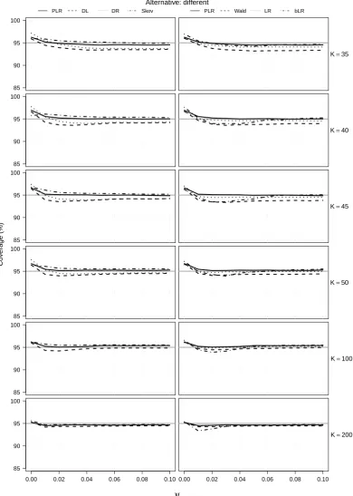
Figure 4 and Figure 5 show the full results from the simulation study in § 4.1 of the paper. Specifically, Figure 4 and Figure 5 include empirical coverage probabilities of two-sided confi-dence intervals for increasing values of ψ for all K ∈ {5,10, . . . ,50,100,200}. The empirical coverage for the double resampling method is computed only for K ≤ 50 because of the long computing times involved. The left column of each figure shows the empirical coverage for the confidence intervals examined in Figure 1 of the main text. The right column shows the em-pirical coverage of confidence intervals based on the Wald statistic, the profile likelihood-ratio statistic, and the Bartlett-corrected likelihood-ratio statistic (see, for example, Huizenga et al., 2011).

3.2 Standardized mean differences from two-arm studies

Figure 6 and Figure 7 show the full results from the simulation study in § 4.2 of the paper. Specifically, Figure 6 and Figure 7 include empirical coverage probabilities of two-sided confi-dence intervals for increasing values of φfor all K ∈ {5,10, . . . ,50,100,200}. The layout of the results in Figure 6 and Figure 7 is the same as that in Figure 4 and Figure 5.

3.3 Case-control study

The current subsection complements§4 of the main text with results from an additional simula-tion study under a more realistic data generating process than the working random-effects meta-analysis model. We assume that theith study consists ofniindividuals, and thatn1, . . . , nK are

independent uniform draws from the integers {30,31, . . . ,100}. Then, conditionally on random effects ui1 and ui2, and covariates xi1, . . . , xinj, we assume that the individual measurements

zi1, . . . , zini in the ith study are realizations of independent Bernoulli random variables with

probabilities exp(ηij)/{1 + exp(ηij)}, where ηij =β0+ui1+ (β1+ui2)xij (j = 1, . . . , ni). The

random effects are assumed to be independent with uit having a N(0, υt) distribution. The

(17)

6

study-specific effectyi is, then, the estimate ofγ2 from a logistic regression with linear predictor

γ1+γ2xij using data (zi1, xi1)>, . . . ,(zini, xini)

>_{. The corresponding estimated variance ˆ}_σ2 i is

based on the evaluation of the expected information matrix at the estimates. The above setting has been inspired by the simulation study in Abo-Zaid et al. (2013, Appendix B). In order to avoid the incidence of infinite estimates, the estimation of the study-specific effects is carried out using thebrglm R package (Kosmidis, 2013).

We useυ1 = 0.1,p= 0.5 and consider a set of “moderate” true effects whereβ0 =−1.27 and

β1 = 0.9, and another set of “larger” effects where β0 =−2 and β1 = 1.5. The between-study

variance υ2 ranges from 0 to 2.5, and the number of studies K ranges from 5 to 200. For each

combination of υ2 and K, 10 000 data sets are simulated. The random number generator is

initialised to have the same state for each combination of υ2 and K.

Figure 8 and Figure 9 show the empirical coverage of various 95% confidence intervals forβ1

under the set of moderate true effects (β0 =−1.27 and β1 = 0.9) for increasing values ofυ2 for

allK ∈ {5,10, ...,50,100,200}. Again, the empirical coverage for the double resampling method

is computed only for K ≤50. Figure 10 and Figure 11 are the corresponding plots for the set of larger true effects (β0 =−2 andβ1= 1.5).

The good performance of the confidence intervals based on the profile penalized likelihood, Skovgaard’s statistic and the Bartlett-corrected likelihood-ratio statistic is apparent for small to moderate number of studies. In contrast, the intervals based on the DerSimonian & Laird estimator, the double bootstrap, the profile likelihood and the Wald statistic illustrate poor performance, particularly for small values ofK. As in Figure 7, Figure 9 and Figure 11 illustrate that as the number of studies grows, model mis-specification eventually results in loss of coverage for all methods examined here, including the one based on the penalized likelihood. The loss of coverage is most severe for small values of the between-variance component υ2. The intervals

based on the DerSimonian & Laird method seem to be the ones most severely affected by model mis-specification.

References

Abo-Zaid, G., Guo, B., Deeks, J. J., Debray, T. P., Steyerberg, E. W., Moons, K. G. & Riley, R. D. (2013). Individual participant data meta-analyses should not ignore clustering. J. Clin. Epidemiol.66, 865–73.

Cooper, N. A. M., Khan, K. S. &Clark T. J. (2010). Local anaesthesia for pain control

during outpatient hysteroscopy: systematic review and meta-analysis. Brit. Med. J. 340, c1130.

Guolo, A. & Varin, C. (2012). The R package metaLik for likelihood inference in

meta-analysis. J. Stat. Softw.50, 1–14.

Huizenga, H. M., Visser, I.&Dolan, C. V. (2011), Testing overall and moderator effects

in random effects meta-regression. Brit. J. Math. Stat. Psy. 64, 1–19.

Kosmidis, I. (2013) brglm: Bias reduction in binary-response Generalized Linear Models. R

package version: 0.5-9, http://www.ucl.ac.uk/ ucakiko/software.html

R Development Core Team (2016). R: A Language and Environment for Statistical

Com-puting. Vienna, Austria: R Foundation for Statistical ComCom-puting. http://www.R-project.org.

Viechtbauer, W. (2005). Bias and efficiency of meta-analytic variance estimators in the

random-effects model. J. Educ. Behav. Stat. 30, 261–93.

(18)

7

ψ

85 90 95 100

ψ

K=5

ψ

85 90 95 100

ψ

K=10

ψ

85 90 95 100

ψ

K=15

ψ

85 90 95 100

ψ

K=20

ψ

85 90 95 100

ψ

K=25

ψ

0.00 0.02 0.04 0.06 0.08 0.10 85

90 95 100

ψ

0.00 0.02 0.04 0.06 0.08 0.10

K=30

Co

v

er

age (%)

ψ

Alternative: different

[image:18.595.107.497.93.641.2]

PLR DL DR Skov PLR Wald LR bLR

(19)

8

ψ

85 90 95 100

ψ

K=35

ψ

85 90 95 100

ψ

K=40

ψ

85 90 95 100

ψ

K=45

ψ

85 90 95 100

ψ

K=50

ψ

85 90 95 100

ψ

K=100

ψ

0.00 0.02 0.04 0.06 0.08 0.10 85

90 95 100

ψ

0.00 0.02 0.04 0.06 0.08 0.10

K=200

Co

v

er

age (%)

ψ

[image:19.595.108.499.101.649.2]

(20)

9

φ

85 90 95 100

φ

K=5

φ

85 90 95 100

φ

K=10

φ

85 90 95 100

φ

K=15

φ

85 90 95 100

φ

K=20

φ

85 90 95 100

φ

K=25

φ

0.0 0.5 1.0 1.5 2.0 2.5 85

90 95 100

φ

0.0 0.5 1.0 1.5 2.0 2.5

K=30

Co

v

er

age (%)

φ

[image:20.595.108.497.101.653.2]

(21)

10

φ

85 90 95 100

φ

K=35

φ

85 90 95 100

φ

K=40

φ

85 90 95 100

φ

K=45

φ

85 90 95 100

φ

K=50

φ

85 90 95 100

φ

K=100

φ

0.0 0.5 1.0 1.5 2.0 2.5 85

90 95 100

φ

0.0 0.5 1.0 1.5 2.0 2.5

K=200

Co

v

er

age (%)

φ

[image:21.595.108.500.101.652.2]

(22)

11

υ2

85 90 95 100

υ2

K=5

υ2

85 90 95 100

υ2

K=10

υ2

85 90 95 100

υ2

K=15

υ2

85 90 95 100

υ2

K=20

υ2

85 90 95 100

υ2

K=25

υ2

0.0 0.5 1.0 1.5 2.0 2.5 85

90 95 100

υ2

0.0 0.5 1.0 1.5 2.0 2.5

K=30

Co

v

er

age (%)

υ2

[image:22.595.107.497.100.649.2]

Figure 8: Empirical coverage probabilities of two-sided confidence intervals for log-odds ratios from a case-control study design with moderate effects. The empirical coverage is calculated for increasing values ofυ2 and forK∈ {5,10,15,20,25,30}. The curves correspond to the proposed

(23)

12

υ2

85 90 95 100

υ2

K=35

υ2

85 90 95 100

υ2

K=40

υ2

85 90 95 100

υ2

K=45

υ2

85 90 95 100

υ2

K=50

υ2

85 90 95 100

υ2

K=100

υ2

0.0 0.5 1.0 1.5 2.0 2.5 85

90 95 100

υ2

0.0 0.5 1.0 1.5 2.0 2.5

K=200

Co

v

er

age (%)

υ2

[image:23.595.108.499.100.648.2]

Figure 9: Empirical coverage probabilities of two-sided confidence intervals for log-odds ratios from a case-control study design with moderate effects. The empirical coverage is calculated for increasing values of υ2 and for K ∈ {35,40,45,50,100,200}. The curves correspond to

(24)

13

υ2

85 90 95 100

υ2

K=5

υ2

85 90 95 100

υ2

K=10

υ2

85 90 95 100

υ2

K=15

υ2

85 90 95 100

υ2

K=20

υ2

85 90 95 100

υ2

K=25

υ2

0.0 0.5 1.0 1.5 2.0 2.5 85

90 95 100

υ2

0.0 0.5 1.0 1.5 2.0 2.5

K=30

Co

v

er

age (%)

υ2

[image:24.595.108.497.100.649.2]

Figure 10: Empirical coverage probabilities of two-sided confidence intervals for log-odds ratios from a case-control study design with larger effects. The empirical coverage is calculated for increasing values ofυ2 and forK∈ {5,10,15,20,25,30}. The curves correspond to the proposed

(25)

14

υ2

85 90 95 100

υ2

K=35

υ2

85 90 95 100

υ2

K=40

υ2

85 90 95 100

υ2

K=45

υ2

85 90 95 100

υ2

K=50

υ2

85 90 95 100

υ2

K=100

υ2

0.0 0.5 1.0 1.5 2.0 2.5 85

90 95 100

υ2

0.0 0.5 1.0 1.5 2.0 2.5

K=200

Co

v

er

age (%)

υ2

[image:25.595.107.500.100.648.2]

Figure 11: Empirical coverage probabilities of two-sided confidence intervals for log-odds ratios from a case-control study design with larger effects. The empirical coverage is calculated for increasing values of υ2 and for K ∈ {35,40,45,50,100,200}. The curves correspond to the