Virtual machine warmup blows hot and cold

(1)

Virtual Machine Warmup Blows Hot and Cold

EDD BARRETT,

King’s College London, UK

CARL FRIEDRICH BOLZ-TEREICK,

REBECCA KILLICK,

Lancaster University, UK

SARAH MOUNT,

LAURENCE TRATT,

Virtual Machines (VMs) with Just-In-Time (JIT) compilers are traditionally thought to execute programs in two phases: the initial warmup phase determines which parts of a program would most benefit from dynamic compilation, before JIT compiling those parts into machine code; subsequently the program is said to be at a steady state of peak performance. Measurement methodologies almost always discard data collected during the warmup phase such that reported measurements focus entirely on peak performance. We introduce a fully automated statistical approach, based on changepoint analysis, which allows us to determine if a program has reached a steady state and, if so, whether that represents peak performance or not. Using this, we show that even when run in the most controlled of circumstances, small, deterministic, widely studied microbenchmarks often fail to reach a steady state of peak performance on a variety of common VMs. Repeating our experiment on 3 different machines, we found that at most 43.5% of⟨VM, benchmark⟩pairs consistently reach a steady state of peak performance.

CCS Concepts: •Software and its engineering→Software performance;Just-in-time compilers; In-terpreters;

Additional Key Words and Phrases: Virtual machine, JIT, benchmarking, performance

ACM Reference Format:

Edd Barrett, Carl Friedrich Bolz-Tereick, Rebecca Killick, Sarah Mount, and Laurence Tratt. 2017. Virtual Machine Warmup Blows Hot and Cold.Draft0, 0, Article 0 (October 2017),40pages.https://arxiv.org/abs/ 1602.00602v6

1 INTRODUCTION

Many modern languages are implemented as Virtual Machines (VMs) which use a Just-In-Time (JIT) compiler to translate ‘hot’ parts of a program into efficient machine code at run-time. Since it takes time to identify and JIT compile the ‘hot’ parts of a program, VMs using a JIT compiler are

said to be subject to awarmupphase. The traditional view of JIT compiled VMs is that program

execution is slow during the warmup phase, and fast afterwards, when asteady stateof peak

performanceis said to have been reached. This traditional view underlies nearly all JIT compiler

benchmarking methodologies: after running benchmarks many times within a single VM process,

∗_{Updates to this paper will be found at}_{https://arxiv.org/abs/1602.00602}

Authors’ URLs: E. Barretthttp://eddbarrett.co.uk/, C. F. Bolz-Tereickhttp://cfbolz.de/, R. Killickhttp://www.lancs.ac.uk/ ~killick/, S. Mounthttp://snim2.org/, L. Tratthttp://tratt.net/laurie/.

Authors’ addresses: Edd Barrett, King’s College London, UK; Carl Friedrich Bolz-Tereick, King’s College London, UK; Rebecca Killick, Lancaster University, UK; Sarah Mount, King’s College London, UK; Laurence Tratt, King’s College London, UK.

Permission to make digital or hard copies of part or all of this work for personal or classroom use is granted without fee provided that copies are not made or distributed for profit or commercial advantage and that copies bear this notice and the full citation on the first page. Copyrights for third-party components of this work must be honored. For all other uses, contact the owner/author(s).

https://arxiv.org/abs/1602.00602v6

(2)

0:2 E. Barrett, C. F. Bolz-Tereick, R. Killick, S. Mount, L. Tratt

the data collected before warmup is discarded, with the reported measurements focussing only on peak performance.

The fundamental aim of this paper is to test, in a highly idealised setting, the following hypothesis:

H1 Small, deterministic programs reach a steady state of peak performance.

To test this hypothesis, we developed a new approach for automatically analysing large quantities of benchmarking data. We deliberately chose widely studied microbenchmarks, and ran them in a heavily controlled environment, designed to minimise measurement noise. By doing so, we maximised the chances that our experiment would validate Hypothesis H1. Instead we encountered many benchmarks which slowdown, never hit a steady state, or have inconsistent performance from one run to the next. Only 30.0–43.5% (depending on the machine and OS combination) of

⟨VM, benchmark⟩pairs consistently reach a steady state of peak performance. Of the seven VMs

we studied, none consistently reached a steady state of peak performance. These results are much worse than reported in previous works.

Our results suggest that much real-world VM benchmarking, which nearly all relies on assuming that benchmarks do reach a steady state of peak performance, is likely to be partly or wholly misleading. Since microbenchmarks similar to those in this paper are often used in isolation to gauge the efficacy of VM optimisations, it is also likely that ineffective, or deleterious, optimisations may have been incorrectly judged as improving performance and included in VMs.

1.1 Overview of the Methodology

We present a carefully designed experiment where benchmarks are run for 2000in-process iterations

and repeated using 30 freshprocess executions(i.e. each process execution runs multiple in-process

iterations). We then automatically analyse and classify the resulting data.

In order to reduce the influence of external factors, we wrote a new benchmarking tool, Krun, to control as many confounding variables as practical. For example, Krun reboots machines before each process execution, turns off or stops network cards and userland daemons, and ensures that the machine’s temperature is consistent before each process execution is run. We ran our experiment on different machines and operating systems to understand the effect of both on benchmarks.

With the time series data produced by Krun, we then encounter the issue of producing useful and reliable summary statistics. Traditional VM benchmarking uses simple heuristics to guess when

warmup has completed, e.g.Georges et al.[2007].Kalibera and Jones[2013] convincingly show the

limitations of such approaches, presenting instead a manual approach to determining if and when a steady state has been reached. While this is a significant improvement on previous methods, it is time-consuming, prone to human inconsistency, and gives no indication as to whether the steady state represents peak performance or not.

We use changepoint analysis [Eckley et al. 2011] to automatically analyse VM benchmarking data.

Changepoint analysis detects shifts in the nature of time series data (e.g. when a benchmark switches from ‘slow’ to ‘fast’ modes after JIT compilation). We then use this information to automatically classify each process execution as either: no steady state; flat (no detectable change in performance

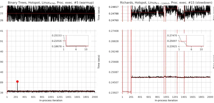
over the benchmark); warmup; or slowdown (a decrease in performance over time). Figure1shows

an example of how changepoint analysis can automatically classify both ‘good’ and ‘bad’ warmup styles. Although simple, these classifications allow us to tease apart unexpected performance patterns that previous methodologies cannot.

Finally, in an attempt to see if there are easy explanations for the odd effects we see, we take two VMs and separate out the time taken to perform Garbage Collection (GC) and JIT compilation. These two factors explain only some of the effects we see.

(3)

1 201 401 601 801 1001 1201 1401 1601 1801 2000

In-process iteration

0.18739 0.19789 0.20840 0.21890 0.22940 0.23991 0.25041

Time (secs)

0.18826 0.18877 0.18927

Time (secs)

Binary Trees, Hotspot, Linux4790, Proc. exec. #5 (warmup)

1 6 10

0.18678 0.21916 0.25153

1 201 401 601 801 1001 1201 1401 1601 1801 2000

0.23927 0.24507 0.25087 0.25668 0.26248 0.26828 0.27408

Time (secs)

0.24760 0.24788 0.24817

Time (secs)

Richards, Hotspot, LinuxE3 − 1240v5, Proc. exec. #15 (slowdown)

1 6 10

[image:3.486.61.434.86.265.2]

0.23925 0.25697 0.27470

Fig. 1. Two example run-sequence plots from our results, augmented with the results of changepoint analysis.

The LHS plot shows an example of ‘traditional’ warmup (in this casebinary treeson HotSpot); the RHS

plot shows an example of slowdown (Richardson HotSpot). The plot titles show: the benchmark (e.g.binary

trees), the VM (e.g. HotSpot), the machine (e.g. Linux4790), the process execution number (e.g. 5), and the

classification (e.g. warmup). The ‘main’ plot at the bottom always shows the in-process iteration number (indexed from 1) and the corresponding wall-clock times for all 2000 in-process iterations. Because this often

obscures the finer details, we also show two additional visualisations of the data: the top plot shares itsxaxis

with the bottom plot, but zooms theyaxis in to where the bulk of the in-process timing data is located; the

smaller inset plot allows us to examine a handful of in-process iteration timings (typically, though not always,

the firstn, allowing us to see the ‘warmup curve’, if it exists). Changepoints are indicated by dashed vertical

red lines and denote a ‘shift’ in performance behaviour; changepoint segments are indicated by dashed horizontal red lines between changepoints, whose height shows the mean iteration time within the segment; and red circles indicate ‘outliers’, which the changepoint analysis discount. We use the changepoint segments to determine if and when a steady state has been reached and, if so, to classify the plots’ warmup style (in this example, warmup and slowdown respectively). As an additional visual aid, changepoint segments considered equivalent in timing to the steady state segment are plotted in black; all other segments are plotted in grey.

1.2 Summary

In summary, this paper’s contributions are as follows:

(1) We show that, even in a highly idealised setting, widely studied benchmarks often fail to reach a steady state of peak performance.

(2) We present the first automated approach to analysing time series data from VM benchmarking, which can automatically determine if and when a steady state has been reached.

(3) We present the first classification of different styles of steady state behaviour (warmup, slowdown, flat).

(4) We show that, while some instances of ‘odd’ behaviour are explained by the ‘obvious’ factors of GC and JIT compilation, many are not.

The statistical approach we have developed is open-source, general, and can be used to analyse any VM benchmarking data. In the Appendix, we show it applied to the DaCapo and Octane

benchmark suites, both run in a conventional manner (AppendixA). We also present a curated

series of plots of interesting data (AppendixC). A separate document contains the complete plots

(4)

Our repeatable experiment, as well as the specific data that forms the basis of this paper’s results, can be downloaded from:

https://archive.org/download/softdev_warmup_experiment_artefacts/v0.8/

2 BACKGROUND

When a program begins running on a JIT compiling VM, it is typically (slowly) interpreted; once ‘hot’ (i.e. frequently executed) loops or methods are identified, they are dynamically compiled into machine code; and subsequent executions of those loops or methods use (fast) machine code rather than the (slow) interpreter. Once machine code generation has completed, the VM is said to have

finished warming up, and the program is said to be executing at a steady state of peak performance.1

While the length of the warmup period is dependent on the program and JIT compiler, all JIT

compiling VMs are based on this performance model [Kalibera and Jones 2013].

Benchmarking of JIT compiled VMs typically focusses on reporting steady state numbers based on two assumptions: first, that warmup is both fast and inconsequential to users; second, that the steady state is also peak performance. The methodologies used are typically straightforward: benchmarks are run for a number of in-process iterations within a single VM process execution.

The firstnin-process iterations are then discarded, on the basis that warmupshouldhave completed

in that period. Oftennis a fixed number (typically around 5), with no guarantee that warmup has

completed by that point. More advanced methods such as that ofGeorges et al.[2007] try to find a

steady state using simple statistical tests.

The most sophisticated VM benchmarking analysis yet developed is found in [Kalibera and Jones

2012,2013]. After showing that simple heuristics such as Georges et al.’s often fail to accurately

pinpoint when warmup has completed, Kalibera and Jones then present an alternative manual process. In essence, after a specific VM / benchmark combination has been run for a small number of process executions, a human must determine if a steady state is reached; and, if it is, at which in-process iteration it is reached. When a steady state does exist, a larger number of in-process executions are then run; the previously determined cut-off point is applied to each process execution’s in-process iterations; and detailed statistics are produced.

The Kalibera and Jones methodology is a significant advance on previous work, and is an important inspiration for ours. However, the reliance on manually identifying when warmup is complete has ramifications. Most obviously, humans are prone to error and disagreement when performing such identifications. More significantly, the time required to manually examine the time series data means that it is only practical to apply it to a small number of initial process executions: the cut-off point that is determined from those is then applied to all future process executions, even though there is no guarantee that they all reach a steady state by that point. With the exception of in-process iterations which show dependence in their data (e.g. a repeated ‘cyclic’ pattern), which are dealt with specially, Kalibera and Jones do not otherwise classify steady state performance relative to what came before it, making it hard to understand if the steady state represents peak performance or not. These three points mean that, despite Kalibera and Jones’s advances, “determining when a system has warmed up, or even providing a rigorous definition of

the term, is an open research problem” [Seaton 2015].

1_{The traditional view applies equally to VMs that perform immediate compilation instead of using an interpreter, and to} those VMs which have more than one layer of JIT compilation (later JIT compilation is used for ‘very hot’ portions of a program, trading slower compilation time for better machine code generation).

(5)

3 METHODOLOGY

To test Hypothesis H1, we designed an experiment which uses a suite of microbenchmarks: each is run with 2000 in-process iterations and repeated using 30 process executions. We have carefully designed our experiment to be repeatable and to control as many potentially confounding variables as is practical. In this section we detail: the benchmarks we used and the modifications we applied; the VMs we benchmarked; the machines we used for benchmarking; and the Krun system we developed to run benchmarks.

First time readers of this paper may find it easiest to jump straight to Section4, coming back to

the complete (lengthy!) methodology on a second read.

3.1 The Microbenchmarks

The microbenchmarks we use are as follows:binary trees,spectralnorm,n-body,fasta, andfannkuch

reduxfrom the Computer Language Benchmarks Game (CLBG) [Bagley et al. 2004]; andRichards.

Readers can be forgiven for initial scepticism about this set of microbenchmarks. They are small and widely used by VM authors as optimisation targets. In general they are more effectively optimised by VMs than average programs; when used as a proxy for other types of programs (e.g. large

programs), they tend to overstate the effectiveness of VM optimisations (see e.g. [Ratanaworabhan

et al. 2009]). In our context, this weakness is in fact a strength: small, deterministic, and widely

examined programs are our most reliable means of testing Hypothesis H1. Put another way, if we were to run arbitrary programs and find unusual warmup behaviour, a VM author might reasonably counter that “you have found the one program that exhibits unusual warmup behaviour”.

For each benchmark, we provide versions in C, Java, JavaScript, Python, Lua, PHP, and Ruby. Since most of these benchmarks have multiple implementations in any given language, we picked

the versions used in [Bolz and Tratt 2015], which represented the fastest performers at the point of

that publication. We lightly modified the benchmarks to integrate with our benchmark runner (see

Section3.5) but did not e.g. force garbage collection.

3.1.1 Ensuring Determinism.User programs that are deliberately non-deterministic are unlikely to warm-up in the traditional fashion. We therefore wish to guarantee that our benchmarks are, to the extent controllable by the user, deterministic, taking the same path through the Control Flow Graph (CFG) on all process executions and in-process iterations. We make no attempt to control non-determinism within the VM, which is part of what we need to test for Hypothesis H1.

To check whether the benchmarks were deterministic at the user-level, we created versions withprintstatements at all possible points of CFG divergence (e.g. inside conditional branches). These versions are available in our experimental suite. We first ran the modified benchmarks with 2 process executions and 20 in-process iterations, and compared the outputs of the two processes.

This was enough to show that thefastabenchmark was non-deterministic in all language variants,

due to its random number generator not being reseeded. We fixed this by moving the random seed initialisation to the start of the in-process iteration main loop.

(6)

3.2 Measuring Computation Rather than File Performance

By their very nature, microbenchmarks tend to perform computations which can be easily opti-mised away. While this speaks well of optimising compilers, benchmarks whose computations are

entirely removed are rarely useful [Seaton 2015]. To prevent optimisers removing such code, many

benchmarks write intermediate and final results tostdout. However, this then means that one

starts including the performance of file routines in libraries and the kernel in measurements, which can become a significant part of the eventual measure.

To avoid this, we modified the benchmarks to calculate a checksum during each in-process iteration. At the end of each in-process iteration the checksum is compared to an expected value;

if the comparison fails then the incorrect checksum is written tostdout. This idiom lowers the

chances that an optimiser can remove the main benchmark code, even though no output is produced. We also use this mechanism to give some assurance that the different language implementations of a benchmark are performing roughly the same work, as the expected checksum value is the same for all implementations of the benchmark.

3.3 VMs under Investigation

We ran the benchmarks on the following language implementations: GCC 4.9.3; Graal 0.18 (an alternative JIT compiler for HotSpot); HHVM 3.15.3 (a JIT compiling VM for PHP); JRuby+Truffle 9.1.2.0 (a JIT compiling VM for Ruby using Graal/Truffle); HotSpot 8u112b15 (the most widely used Java VM); LuaJIT 2.0.4 (a tracing JIT compiling VM for Lua); PyPy 5.6.0 (a meta-tracing JIT compiling VM for Python 2.7); and V8 5.4.500.43 (a JIT compiling VM for JavaScript). A repeatable build script downloads, patches, and builds fixed versions of each VM. All VMs were compiled with GCC/G++ 4.9.3 (and GCC/G++ bootstraps itself, so that the version we use compiled itself) to remove the possibility of variance through the use of different compilers.

We skipped: Graal, HHVM, and JRuby+Truffle on OpenBSD, as these VMs have not yet been

ported to this platform;fastaon JRuby+Truffle as it crashes; andRichardson HHVM since it takes

as long as every other benchmark on every other VM put together.

3.4 Benchmarking Hardware

With regards to hardware and operating systems, we made the following hypothesis:

H2 Moderately different hardware and operating systems have little effect on warmup.

We deliberately use the word ‘moderately’, since significant changes of hardware (e.g. x86 vs. ARM) or operating system (e.g. Linux vs. Windows) imply that significantly different parts of the VMs

will be used (see Section7).

In order to test Hypothesis H2, we used three benchmarking machines:Linux1240v5, a Xeon

E3-1240 v5 3.5GHz, 24GB of RAM, running Debian 8;Linux4790, a quad-core i7-4790 3.6GHz, 32GB

of RAM, running Debian 8; andOpenBSD4790, a quad-core i7-4790 3.6GHz, 32GB of RAM, running

OpenBSD 6.0. Linux1240v5and Linux4790have the same OS (with the same packages and updates

etc.) but different hardware; Linux4790and OpenBSD4790have the same hardware (to the extent we

can determine) but different operating systems.

We disabled turbo boost and hyper-threading in the BIOS. Turbo boost allows CPUs to tem-porarily run in an higher-performance mode; if the CPU deems it ineffective, or if its safe limits

(e.g. temperature) are exceeded, turbo boost is reduced [Charles et al. 2009]. Turbo boost can thus

substantially change one’s perception of performance. Hyper-threading gives the illusion that a single physical core is two logical cores. Programs and threads that would otherwise run on separate physical cores are thus inter-leaved on a single core, leading to less predictable performance.

(7)

3.5 Krun

Many confounding variables manifest shortly before, or during the running of, benchmarks [

Kalib-era et al. 2005]. In order to control as many of these as possible, we wrote Krun2. Krun is a

‘supervisor’ which, given a configuration file specifying VMs, benchmarks, etc. configures a Linux or OpenBSD system, runs benchmarks, and collects the results. Individual VMs and benchmarks are then wrapped, or altered, to report data back to Krun in an appropriate format.

In the remainder of this subsection, we describe Krun. Since most of Krun’s controls work identically on Linux and OpenBSD, we start with those, before detailing the differences imposed by the two operating systems. We then describe how Krun collects data from benchmarks. Note that, although Krun has various ‘developer’ flags to aid development and debugging benchmarking suites, we describe only Krun’s full ‘production’ mode.

3.5.1 Platform Independent Controls.A typical problem with benchmarking is that earlier process executions can affect later ones (e.g. a benchmark which forces memory to swap will make later benchmarks seem to run slower). Therefore, before each process execution (including before the first), Krun reboots the system, ensuring that each process execution runs with the machine in a state that is uninfluenced by previous process executions. After each reboot, Krun is executed by the init subsystem; Krun then pauses for 3 minutes to allow the system to fully initialise; calls

sync(to flush any remaining files to disk) followed by a 30 second wait; before finally running the

next process execution.

The obvious way for Krun to determine which benchmark to run next is to examine its results file. However, this is a large file which grows over time, and reading it in could affect benchmarks (e.g. due to significant memory fragmentation). When invoked for the first time, Krun creates a simple schedule file. After each reboot this is scanned line-by-line for the next benchmark to run; the benchmark is run; and the schedule updated, without changing its size. Once the process execution is complete, Krun can safely load the results file in and append the results data, knowing that the reboot that will occur shortly after will put the machine into a (largely) known state.

Modern systems have various temperature-based limiters built in: CPUs, for example, lower their frequency if they get too hot. After its initial invocation, Krun waits for 1 minute before

collecting the values of all available temperature sensors. After each reboot’ssync-wait, Krun

waits for the machine to return to these base temperatures (±3°C) before starting the benchmark,

fatally aborting if this temperature range is not met within 1 hour. In so doing, we aim to lessen the impact of ambient temperature changes.

Krun fixes the heap and stackulimitfor all VM processes (in our case, 2GiB heap and a 8MiB

stack).3_{Benchmarks are run as the ‘}_krun_{’ user, whose account and home directory are created}

afresh before each process execution to prevent cached files affecting benchmarking.

User-configurable commands can be run before and after each process execution. We disabled as many Unix daemons as possible (e.g. smtpd, crond) to lessen the effects of context switching. We also turned off network interfaces entirely, to prevent outside sources causing (potentially performance interfering) interrupts to be sent to the processor and kernel.

In order to identify problems with the machine itself, Krun monitors the systemdmesgbuffer

for unexpected entries (known ‘safe’ entries are ignored), informing the user if any arise. We im-plemented this after noticing that one machine initially ear-marked for benchmarking occasionally

overheated during benchmarking, with the only clue to this being a line indmesg. We did not use

this machine for our final benchmarking.

2_{The ‘K’ in Krun is a respectful tip of the hat to Kalibera and Jones.}

(8)

A process’s environment size can cause measurement bias [Mytkowicz et al. 2009]. The diversity

of VMs and platforms in our setup makes it impossible to set a unified environment size across

all VMs and benchmarks. However, thekrunuser does not vary its environment (we recorded

the environment seen by each process execution and verified their size), and we designed the

experiment such that, for each machine, each⟨VM, benchmark⟩has a consistent environment size.

3.5.2 Linux-specific Controls.On Linux, Krun controls several additional factors, sometimes by checking that the user has correctly set controls which can only be set manually.

Krun usescpufreq-setto set the CPU governor toperformancemode (i.e. the highest

non-overclocked frequency possible). To prevent the kernel overriding this setting, Krun verifies that

the user has disabled Intel P-state support in the kernel by passingintel_pstate=disable

as a kernel argument.

As standard, Linux interrupts (‘ticks’) each coreCONFIG_HZtimes per second (usually 250) to

decide whether to perform a context switch. To avoid these repeated interruptions, Krun checks

that it is running on a ‘tickless’ kernel [Linux 2013], which requires recompiling the kernel with

theCONFIG_NO_HZ_FULL_ALLoption set. Whilst the boot core still ‘ticks’, other cores only ‘tick’ if more than one runnable process is scheduled.

Similarly, Linux’sperfprofiler may interrupt cores up to 100,000 times a second. We became

aware ofperfwhen Krun’sdmesgchecks notified us that the kernel had decreased the

sample-rate by 50% due to excessive overhead. While frequent sampling will clearly have some performance impact, adaptive sampling is even more troubling: a change of sample rate during a process execution

could notably change performance. Althoughperfcannot be completely disabled, Krun sets it to

sample at most once per second, minimising interruptions.

3.5.3 OpenBSD-specific Controls.Relative to Linux, OpenBSD exposes fewer controls to user. Nevertheless, there are two OpenBSD specific features in Krun. First, Krun sets CPU

perfor-mance to maximum by invokingapm -Hprior to running benchmarks (equivalent to Linux’s

performancemode). Second, Krun minimises the non-determinism in OpenBSD’s malloc

imple-mentation, for example not requiringreallocto always reallocate memory to an entirely new

location. Themalloc.confflags we use arecfgrux.

3.5.4 The Iteration Runners. To report timing data to Krun, we created aniteration runnerfor each language under investigation. These take the name of a specific benchmark and the desired number of in-process iterations, run the benchmark appropriately, and once it has completed, print

the times tostdoutfor Krun to capture. For each in-process iteration we measure (on Linux and

OpenBSD) the wall-clock time taken, and (Linux only) core cycle, APERF, and MPERF counters.

We use a monotonic wall-clock timer with sub-millisecond accuracy (CLOCK_MONOTONIC_RAW

on Linux, andCLOCK_MONOTONICon OpenBSD). Although wall-clock time is the only measure

which really matters to users, it gives no insight into multi-threaded computations: on Linux we also

record core-cycle counts using theCPU_CLK_UNHALTED.COREcounter to see what work each

core is actually doing. In contrast, we use the ratio of APERF/MPERF deltas solely as a safety check

that our wall-clock times are valid. TheIA32_APERFcounter increments at a rate proportional to

the processor’s current frequency; theIA32_MPERFcounter increments at a fixed rate normalised

to the CPU’s base frequency. With an APERF/MPERF ratio of precisely 1, the processor is running at full speed; below 1 it is in a power-saving mode; and above 1, turbo boost is being used.

A deliberate design goal of the in-process iteration runners is to minimise timing noise and distortion from measurements. Since system calls can have a significant overhead (on Linux, calling

functions such aswritecan evict as much as two thirds of an x86’s L1 cache [Soares and Stumm

2010]), we avoid making any system calls other than those required to take measurements. We

(9)

void krun_measure(int mdata_idx) {

struct krun_data *data = &(krun_mdata[mdata_idx]); if (mdata_idx == 0) { // start benchmark readings

for (int core = 0; core < num_cores; core++) { data->aperf[core] = read_aperf(core); data->mperf[core] = read_mperf(core);

data->core_cycles[core] = read_core_cycles(core); }

data->wallclock = krun_clock_gettime_monotonic(); } else { // end benchmark readings

data->wallclock = krun_clock_gettime_monotonic(); for (int core = 0; core < num_cores; core++) {

data->core_cycles[core] = read_core_cycles(core); data->aperf[core] = read_aperf(core);

data->mperf[core] = read_mperf(core); }

} }

wallclock_times = [0] * iters for i in xrange(iters):

# Start timed section krun_measure(0) # Call the benchmark bench_func(param) # End timed section krun_measure(1) wallclock_times[i] = \

krun_get_wallclock(1) - \ krun_get_wallclock(0) js = { "wallclock_times": \

wallclock_times } sys.stdout.write(\

"%s\n" % json.dumps(js))

Listing 1. krun_measure: Measuring before (theiftrue

branch) and after (the false branch) a benchmark. Since wall-clock time is the most important measure, it is innermost; since the APERF/MPERF counters are a sanity check, they are outermost. Note that the APERF/MPERF counters must be read in the same order before and after a benchmark.

Listing 2. An elided version of the Python in-process iteration runner (with core-cycles etc. removed).

avoid in-benchmark I/O and memory allocation by storing measurements in a pre-allocated buffer

and only writing measurements tostdoutafter all in-process iterations have completed (see

Listing2for an example). However, the situation on Linux is complicated by our need to read

core-cycle and APERF/MPERF counts from Model Specific Register (MSR) file device nodes,4which

are relatively slow (see Section7). Since wall-clock time is the most important measure, we ensure

that it is the innermost measure taken (i.e. to the extent we control, it does not include the time

taken to read core-cycle or APERF/MPERF counts) as shown in Listing1.

The need to carefully sequence the measurements, and the fact that not all of the VMs in our experiment give us access to the appropriate monotonic timer, meant that we had to implement a

small C library (libkruntime.so) to do so (see Listing1for an example). When possible (all

VMs apart from JRuby+Truffle, HHVM, and V8), we used a language’s FFI to dynamically load this library; in the remaining cases, we linked the library directly against the VM, which then required us to add user-language visible functions to access them. Core-cycle, APERF, and MPERF counts are 64-bit unsigned integers; since JavaScript and current versions of LuaJIT do not support integers, and since PHP’s maximum integer size varies across OS and PHP versions, we convert the 64-bit unsigned measurements to double-precision floating point values in those VMs, throwing an error if this leads to a loss of precision.

4 CLASSIFYING WARMUP

The main data created by our experiment is the time taken by each in-process iteration to run. Formally, this is time series data of length 2000. In this Section we explain how we use statistical changepoint analysis to enable us to understand this time series data and classify the results we see, giving the first automated method for identifying warmup.

(10)

4.1 Outliers

As is common with analyses of time series data, we first identifyoutliers(in-process iterations with

much larger/smaller times than their near neighbours), which in our context are likely to be the result of JIT compilation, GC, or of other processes interrupting benchmarks. Outliers can then be ignored when looking for meaningful performance shifts during changepoint analysis. We use the

method described byTukey[1977], conservatively defining an outlier as one that, within a sliding

window of 200 in-process iterations, lies outside the median±3× (90%ile−10%ile). In order that

we avoid classifying slow warmup iterations at the start of an execution as outliers (when they are in fact likely to be important warmup data), we ignore the first 200 in-process iterations. Of the

7,320,000 in-process iterations, 0.3% are classified as outliers, with the most for any single process

execution being 11.2% of in-process iterations.

4.2 Changepoint Analysis

Intuitively, in order to uncover if/when warmup has completed, we need to determine when in-process iteration timings have ‘shifted’ in nature (i.e. become faster or slower). For example, for

traditional warmup, we would expect to see a number of in-process iterations taking timetto be

followed by a number at timet′_(where_t′_<_{t). Automating the detection of such ‘shifts’ is tricky:}

simple heuristics suffer from both false positives and negatives [Kalibera and Jones 2013]; and ‘I

know it when I see it’ manual detection is time-consuming and prone to human error.

Instead, we use changepoint analysis (seeEckley et al.[2011] for an introduction) to determine

if and when warmup has occurred. Formally, achangepointis a point in time where the statistical

properties of prior data are different to the statistical properties of subsequent data; the data between

two changepoints is achangepoint segment. Changepoint analysis is a computationally

challeng-ing problem, requirchalleng-ing consideration of large numbers of possible changepoints. A completely

naive approach requires an infeasible 2n−1calculations (21999in our context). More sophisticated

changepoint analysis algorithms reduce this toO(n3). We utilise the PELT algorithm [Killick et al.

2012] which reduces the complexity toO(n)by noting that once an ‘obvious’ changepoint has been

discovered, it is not worth including data before that changepoint in further searches.

There are various ways of defining when a changepoint has occurred, but the best fit for our data is to consider changes in both the mean and variance of in-process iterations. To automate this,

we use thecpt.meanvarfunction in the Rchangepointpackage [Killick and Eckley 2014],

passing 15 logn(wherenis the time series length minus the number of outliers) to thepenalty

argument, and receiving back changepoint locations along with the mean and variance of each changepoint segment. Whilst dependence is observed in some of our experiment’s data, the large

penalty we use allows us to make an assumption of independence [Antoch et al. 1997] (see Section7

for details). Figure1shows an example of changepoints and changepoint segments in our context.

4.3 Classifications

Building atop changepoint analysis, we can then define useful classifications for time series data from VM benchmarks.

However, we must first acknowledge the constraints that changepoint analysis works under: it has no way of knowing what constitutes the ‘noise floor’ in our problem domain; nor can it guarantee to find identical means for very similar segments separated from one another by a segment with a clearly distinct mean or variance. To understand how the ‘noise floor’ affects our analysis, it is helpful to take an extreme example. Consider a long sequence of in-process iterations all timed at 0.1001 seconds, followed by another long sequence timed at 0.1002 seconds. A changepoint will be detected in the transition between the two sequences, resulting in two

(11)

DELTA = 0.001 # Absolute time delta (in seconds) below which segments are # considered equivalent.

STEADY_STATE_LEN = 500 # How many in-process iterations from the end of the time-series # data will a non-equivalent segment trigger "no steady state"?

def classify(segs): assert(len(segs) > 0)

last_seg = segs[len(segs) - 1]

lower_bound = last_seg.mean - max(last_seg.variance, DELTA) upper_bound = last_seg.mean + max(last_seg.variance, DELTA) cls = "flat"

i = len(segs) - 2 while i > -1:

cur_seg = segs[i] i -= 1

if cur_seg.mean + cur_seg.variance >= lower_bound \ and cur_seg.mean - cur_seg.variance <= upper_bound:

continue

elif cur_seg.end > len(segs) - STEADY_STATE_LEN: cls = "no steady state"

break

elif cur_seg.mean < lower_bound: cls = "slowdown"

break

assert(cur_seg.mean > upper_bound) cls = "warmup"

return cls

Listing 3. The classification algorithm for an individual process execution. Given an ordered list of segments (each with "mean", "variance", and "end" attributes, the latter being the absolute index of the last iteration in the segment) this function returns a string classifying the run sequence’s warmup style.

changepoint segments. However, we know that in practice such a small absolute timing delta is as likely to be the result of non-determinism inherent in a real machine or OS as it is to be due to a benchmark or VM: it would thus be better to consider the two segments as being equivalent. Such segments are not always contiguous. Consider a benchmark which, after changepoint analysis, has three segments: the first with a mean of 1.0001 seconds, the second 1.2 seconds (perhaps whilst a JIT compiler is in action), the third 1.0002 seconds. From our perspective, the first and final segments are best considered as being equivalent, even though they are separated by a segment which is clearly different. We therefore need to define a suitable tolerance for determining if two segments are equivalent. In short running benchmarks, a small number of external events can add an absolute level of noise: in our experience readings often vary by a little under 0.001s. In long running benchmarks, an individual external event may add a relatively small amount of noise, but the cumulative effect of many external events can add up. We found that the variance was a good heuristic for this cumulative effect (we simply interpreted it as having units in seconds rather

than seconds squared). Combining these two notions, we thus formally define that a segmentsiis

equivalent to the final segmentsf if mean(si)is within mean(sf) ±max(variance(sf),0.001s).

With that in mind, we can define a simple classification algorithm for a process execution, based on the special nature of the final changepoint segment. Since all our benchmarks run for 2000 in-process iterations we (somewhat arbitrarily) define that a in-process execution reaches a steady-state if all segments which cover the last 500 in-process iterations are considered equivalent to the final

segment. If not, we classify the process execution asno steady state( ). If a steady state is reached, we

are then interested as to whether: all segments are considered equivalent, leading to a classification

offlat( ); at least one segment is faster than the final segment leading to a classification ofslowdown

( ). If a steady state benchmark is not flat or a slowdown, then by definition the final segment must

(12)

shows an implementation of this algorithm. We consider benchmarks whose behaviour is either flat or warmup as ‘good’ (flat benchmarks may be unobservably fast warmup), while benchmarks which are either slowdown or no steady state as ‘bad’.

Based on this, we can then classify a⟨VM, benchmark⟩pair as follows: if its process executions

all share the same classification (e.g. warmup) then we classify the pair the same way (in this

example, warmup); otherwise we classify the pair asinconsistent. There are then two sub-categories

of inconsistent benchmarks: ‘good’ inconsistency ( ) is where all a⟨VM, benchmark⟩pair’s process

executions are either flat or warmup; and ‘bad’ inconsistency ( ) is when one or more process exe-cutions are no steady state or slowdown. Good inconsistency can occur because some benchmarks are on the edge of our ability to differentiate warmup from flat behaviour, and we prefer to assume that we are at fault rather than the VM. Bad inconsistency is always more troubling: it means that, at least sometimes, users will experience poor performance.

4.4 Steady State Timings

For benchmarks whose process executions all reach a steady state (i.e. are any combination of , ,

or ) we report the number of iterations (steady iter (#)) and the time in seconds (steady iter (s)) to

reach the steady state, as well as the performance within the steady state (steady perf (s)).

Steady iter (#)andsteady iter (s)allow one to understand how long it takes a benchmark to reach

a steady state, and are made possible by our use of changepoint analysis. Flat process executions by

definition have asteady iter (#)of 1 and asteady iter (s)of 0; we elide these details for benchmarks

which are consistently flat. Benchmarks often end up with a variety of distributions for both these measures (often, though not exclusively, seen on benchmarks which contain a mix of flat and non-flat classifications) which makes reporting standard confidence intervals misleading. We therefore use Inter-Quartile Ranges (IQRs) to give an indication of the spread of values, reporting the median and 5% and 95% percentiles (using linear interpolation when the percentile boundaries

lie between two data points). Non-overlapping IQRs imply a meaningful difference in thesteady

iter (#)or(s)values of a benchmark run on two VMs; however, since IQRs are often widely spread,

we are not always able to prove meaningful differences. To give a more nuanced view than IQRs can report we also provide thumbnail histograms.

Steady perf (s)roughly corresponds to the ‘normal’ performance number reported by traditional

benchmarking methodologies. In our case, the steady state is composed of one or more segments

(see Section4.3). We report means and 99% confidence intervals calculated via bootstrapping (with

100,000 iterations). Although we assume that values within segments are independent (see Section7),

the values across different segments are clearly not independent. When bootstrapping, we therefore

sample values within, but never across, segments (e.g. if a steady state has two segmentsAand

B, we bootstrapAto produceA′andBto produceB′; we then mergeA′andB′to produce a new

(bootstrapped) steady state; we never sample values fromAintoB′orBintoA′).

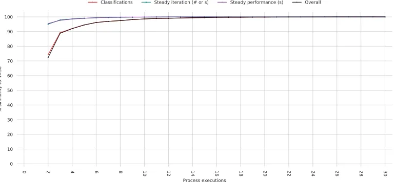
5 RESULTS

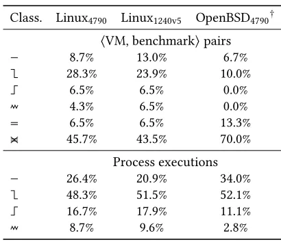
Our results consist of data for 3660 process executions and 7,320,000 in-process iterations. Table1

summarises the⟨VM, benchmark⟩pairs and process executions for each benchmarking machine.

Taking Linux1240v5as a representative example, 43.4% of⟨VM, benchmark⟩pairs have consistently

‘good’ warmup (i.e. are flat, warmup, or good inconsistent) and 72.4% of all process executions

have ‘good’ warmup (for comparison, Linux4790is 43.5% and 74.7% respectively and OpenBSD4790is

30.0% and 86.1% respectively, though the latter runs fewer benchmarks). Fewer⟨VM, benchmark⟩

pairs than process executions have ‘good’ warmup because some inconsistent⟨VM, benchmark⟩

pairs have some ‘good’ warmup process executions as well as some ‘bad’. On Linux1240v56.5% of

⟨VM, benchmark⟩pairs slowdown, 6.5% of⟨VM, benchmark⟩pairs are no steady state, but the

(13)

Class. Linux4790 Linux1240v5 OpenBSD4790†

⟨VM, benchmark⟩pairs

8.7% 13.0% 6.7%

28.3% 23.9% 10.0%

6.5% 6.5% 0.0%

4.3% 6.5% 0.0%

6.5% 6.5% 13.3%

45.7% 43.5% 70.0%

Process executions

26.4% 20.9% 34.0%

48.3% 51.5% 52.1%

16.7% 17.9% 11.1%

[image:13.486.139.344.83.260.2]

8.7% 9.6% 2.8%

Table 1. Relative proportions of classifiers across benchmarking machines. Classifiers key: : flat, : warmup,

: slowdown, : no steady state, : good inconsistent, : bad inconsistent.†Note that Linux4790 and

Linux1240v5run the same set of benchmarks, but OpenBSD4790runs a subset (see Section3.3).

biggest proportion by far is ‘bad’ inconsistent at 43.5% (Linux4790has very similar proportions).

This latter figure clearly shows a widespread lack of predictability: in almost half of cases, the same benchmark on the same VM on the same machine has more than one performance characteristic. It is tempting to pick one of these performance characteristics – VM benchmarking sometimes

reports the fastest process execution, for example – but it is important to note thatallof these

performance characteristics are valid and may be experienced by real-world users.

Table1clearly shows that the results from Linux1240v5and Linux4790(both running Linux but on

quite different hardware) are comparable, with the relative proportions of all measures being only

a few percent different. OpenBSD4790(running a different OS to Linux4790, but on similar hardware)

is however fairly different, with 70.0% of⟨VM, benchmark⟩pairs being ‘bad’ inconsistent. This is

partly due to the absence of JRuby+Truffle which, on Linux, is the most consistent (see Section3.3).

Of the benchmarks OpenBSD4790can run, most behave roughly similarly (as can be seen indirectly

from Table1), but there is a more even spread of process execution classifications across⟨VM,

benchmark⟩pairs. Tables8and9in the Appendix contain further details. Overall, we believe that

our results are a somewhat clear validation of Hypothesis H2.

Looking at one machine’s data brings out further detail. For example, Table2(with data from

Linux1240v5) enables us to make several observations. First, of the 6 benchmarks, only n-body

andspectralnormcome close to ‘good’ warmup behaviour on all VMs (though each has 1 or 2

bad inconsistent cases). Second,binary treesseems generally to be bad inconsistent, andfasta

andRichardsoften bad inconsistent. This raises the question as to whether some aspect of these

(14)

0:14 E. Barr ett, C. F . Bolz-T er eick, R. Killick, S. Mount, L. T ratt

Steady Steady Steady Steady Steady Steady Class. iter (#) iter (s) perf (s) Class. iter (#) iter (s) perf (s) C binar y tr ees n-b ody

0.40555 ±0.005110

Graal (27,3 ) ₍₁₇_.₀_,₁₉₃32_..₈₎0 ₍₃_.₇₂₉_,₃₆6_.₆₀₈₎.60 _±00._.18594₀₀₀₃₁₅ ₍₇_.₅_,8₈_..₅₎0 ₍₁_.₁₂₆_,₁1_..₃₅₈₎22 0_±0.13334_.₀₀₀₀₄₅

HHVM (24,4 ,2 ) (16,11 ,3 )

HotSpot (25,5 ) ₍₇_.₀_,₅₃7_..₅₎0 ₍₁_.₁₈₂_,₉1_.₇₀₃₎.19 _±00._.18279₀₀₀₁₁₆ ₍₂_.₀_,2₂_..₀₎0 ₍₀_.₁₄₁_,₀0_..₁₄₃₎14 0_±0.13699_.₀₀₀₀₃₂

JRuby+Truffle 1082.0

(999.0,1232.5) 2219

.59

(2039.304,2516.021) 2

.05150

±0.017738 69

.0

(69.0,70.0) 17

.95

(17.716,18.127) 0

.20644 ±0.001568

LuaJIT (23,4 ,2 ,1 ) 0_±0.25399_.₀₀₄₄₇₁

PyPy (27,3 ) 1_±0.85835_.₀₁₂₈₉₃

V8 (15,9 ,6 ) ₍₁_.₀_,₇₉₄1_..₀₎5 ₍₀_.₀₀₀_,₃₉₁0_.₀₂₆₎.25 _±00._.49237₀₀₃₁₉₈ (25,5 ) ₍₁_.₀_,₃₆₁1_..₆₎0 ₍₀_.₀₀₀_,₈₇0_..₃₆₇₎00 0_±0.24138_.₀₀₀₃₈₉

C

fannkuch

re

dux

(21,6 ,2 ,1 )

Richar

ds

(19,5 ,4 ,2 )

Graal (28,1 ,1 ) (28,1 ,1 )

HHVM 10.0

(10.0,10.0) (52.660,5252.708).66 ±01.35779.011948

HotSpot 390.0

(2.0,390.0) (0.407,153155.254).70 ±00.36202.022767 (26,2 ,2 )

(999.0,1023.1) (1014.290,10391059.967).04 ±01.08833.038580 (1014.91021,1027..0)0 (901.708,946917..683)30 0±0.89509.027590

LuaJIT 0.56285

±0.000097 (21,7 ,2 )

PyPy (15,13 ,2 ) ₍₁_.₀_,₂₈2_..₉₎0 ₍₀_.₀₀₀_,₄₃1_.₄₈₃₎.57 _±01.55442_.₀₂₀₅₄₉ ₍₂_.₀_,2₅_..₀₎0 ₍₁_.₁₁₄_,₄1_.₀₅₄₎.12 0_±0.96809_.₀₁₀₉₅₀

V8 (19,11 ) ₍₁_.₀_,₂₅2_..₅₎0 ₍₀_.₀₀₀_,₇0_.₅₂₅₎.31 _±00.30401_.₀₀₀₁₅₄ (29,1 ) ₍₄_.₀_,₁₆4_..₀₎0 ₍₁_.₄₃₄_,₇1_..₁₃₅₎44 0_±0.47421_.₀₀₁₂₁₈

C

fasta

0.07048 ±0.000210

sp

ectralnorm

(28,1 ,1 ) ₍₂_.₀_,₁₀₀₁997_..₀₎0 ₍₀_.₅₄₆_,546₅₄₇_..₇₁₇₎38 0_±0.54547_.₀₀₂₅₆₂

Graal (29,1 ) (29,1 ) ₍₂_.₀_,15₂₁_..₀₎0 ₍₀_.₈₁₂_,₁₇12_..₈₀₄₎40 0_±0.89293_.₀₀₀₀₈₇

HHVM (27,2 ,1 ) ₍₃₄_.₀_,35₄₁_..₀₎0 ₍₁₃₆_.₉₀₉_,139₁₄₇_..₆₂₆₎18 1_±0.40690_.₀₁₁₁₃₃

HotSpot (18,12 ) ₍₆_.₀261_,₅₉₅_..₀₎0 ₍₀_.₆₁₄_,₇₀30_.₀₂₁₎.73 _±00._.11744₀₀₁₇₂₃ ₍₇_.₀_,7₈_..₆₎0 ₍₁_.₉₀₁_,₂1_..₄₂₅₎90 0_±0.31470_.₀₀₀₀₂₉

(1007.5,1014.0) (888.985,893896..562)38 0±0.83633.014403

LuaJIT 0.22435

±0.000020

PyPy 75.0

(75.0,75.0) (34.429,3434..437)43 0±0.46489.000046

[image:14.486.78.637.38.387.2]

V8 (19,10 ,1 ) ₍₃_.₀_,3₃_..₀₎0 ₍₀_.₅₅₄_,₀0_..₅₅₄₎55 0_±0.24963_.₀₀₀₀₃₉

Table 2. Results for Linux1240v5. We report the classification of each process execution and, for inconsistent benchmarks, the constituent classifications (e.g.

(22 , 8 ) means 22 slowdowns and 8 warmups). If a steady state is achieved, we report three summary statistics.Steady iter (#)is the median in-process

iteration number to reach the steady state, andSteady iter (s)is the median wall-clock time (since the beginning of the process execution) to reach the steady

state; for both measures we report 5% and 95% inter-quartile ranges.Steady perf (s)is the mean steady state performance across all process executions

(reported with 99% confidence intervals). Thumbnail histograms show the spread of values; the red bars indicates the median values.

(15)

1 201 401 601 801 1001 1201 1401 1601 1801 2000 In-process iteration 0.49034 0.49320 0.49607 0.49893 0.50180 0.50466 0.50753 Time (secs) 0.000×109 0.909×109 1.817×109 CC #0

Binary Trees, V8, Linux4790, Proc. exec. #24 (no steady state)

0.000×109 0.909×109 1.817×109 CC #1 0.000×109 0.909×109 1.817×109 CC #2 0.000×109 0.909×109 1.817×109 CC #3

1 26 50

[image:15.486.49.235.86.255.2]

0.49764 0.50266 0.50769

Fig. 2. An example of a run-sequence plot with core-cycle plots (one for each of the 4 CPU cores; note that

they all have the sameyaxis scale). In this example we

can clearly see a benchmark migrating between cores. In some cases this migration also aligns with a clear changepoint, though not in others. The continual changepoints lead to an overall classification of no steady state.

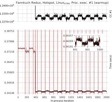
1 201 401 601 801 1001 1201 1401 1601 1801 2000

In-process iteration 0.34148 0.34916 0.35683 0.36451 0.37218 0.37986 0.38753 Time (secs) 1.2270×109 1.2335×109 1.2400×109 CC #1

Fannkuch Redux, Hotspot, Linux4790, Proc. exec. #1 (warmup)

601 801 1000

[image:15.486.253.437.88.256.2]

0.34181 0.34269 0.34357

Fig. 3. Cycles in wall-clock times which are reflected by the core-cycle count for the relevant core. Al-though the changepoint analysis has captured the cycles, the change in performance is too small for the classification algorithm to consider this example ‘no steady state’.

1 201 401 601 801 1001 1201 1401 1601 1801 2000

In-process iteration 0.49007 0.49149 0.49290 0.49432 0.49573 0.49714 0.49856 Time (secs)

Binary Trees, V8, LinuxE3 − 1240v5, Proc. exec. #7 (warmup)

1 201 401 601 801 1001 1201 1401 1601 1801 2000

Binary Trees, V8, LinuxE3 − 1240v5, Proc. exec. #8 (slowdown)

1 26 50

0.49013 0.49409 0.49806

1 26 50

0.49179 0.49523 0.49867

Fig. 4. An example of bad inconsistency: the same benchmark, on the same VM, on the same machine, with one process execution warming up and the other slowing down.

5.1 Warmup Plots

We created several different types of plot to help us understand our data in detail. All plots have

in-process iteration number on thex-axis. Run-sequence plots show wall-clock times on they-axis.

The plots in Figure1show run-sequence plots for warmup and slowdown behaviours. Figure4

shows an example of bad inconsistency and Figure5of good inconsistency. Core-cycle plots (Linux

only) show the core-cycle counts on they-axes (one plot per-core). The plots in Figures2and3

[image:15.486.52.439.376.515.2]

(16)

1 201 401 601 801 1001 1201 1401 1601 1801 2000

Binary Trees, PyPy, OpenBSD4790, Proc. exec. #24 (warmup)

1 201 401 601 801 1001 1201 1401 1601 1801 2000

Binary Trees, PyPy, OpenBSD4790, Proc. exec. #28 (flat)

1 7 12

1.14687 1.17782 1.20876

1 7 12

[image:16.486.50.438.84.225.2]

1.14754 1.17497 1.20240

Fig. 5. An example of good inconsistency where one process execution is classified as warmup, the other flat. Although a human might consider both of these as warmup, there is a subtle difference in the nature of the first 20–30 in-process iterations in the LHS and RHS plots, which leads changepoint analysis to consider the RHS plot as a single changepoint segment.

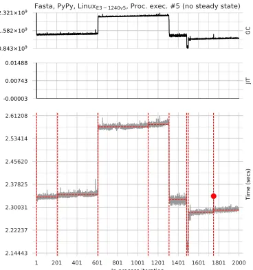
1 201 401 601 801 1001 1201 1401 1601 1801 2000

In-process iteration 2.14443 2.22237 2.30031 2.37825 2.45620 2.53414 2.61208 Time (secs) 0.843×109 1.582×109 2.321×109 GC

Fasta, PyPy, LinuxE3 − 1240v5, Proc. exec. #5 (no steady state)

-0.00003 0.00743 0.01488

JIT

Fig. 6. A run-sequence plot (bottom) with GC (top) and JIT (middle) plots. In this case, the benchmark’s gradually increasing wall-clock time clearly correlates with GC. This example (along with several others) appears to show a memory leak in PyPy, which we have reported upstream.

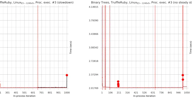
1 201 401 601 801 1001 1201 1401 1601 1801 2000

In-process iteration 0.24492 0.25075 0.25657 0.26239 0.26821 0.27403 0.27985 Time (secs) -0.00000 0.00050 0.00100 GC (secs)

Richards, Hotspot, LinuxE3 − 1240v5, Proc. exec. #3 (slowdown)

-0.00008 0.01950 0.03908

JIT (secs)

1 26 50

[image:16.486.252.438.292.493.2]

0.24451 0.26249 0.28047

Fig. 7. Slowdown at in-process iteration #199, which correlates with two immediately preceding JIT com-pilation events that may explain the drop in perfor-mance. Note that the regular GC spikes have only a small effect on wall-clock time.

Core-cycle plots help us understand how VMs use, and how the OS schedules, threads. Bench-marks running on single-threaded VMs are characterised by a high cycle-count on one core, and very low (though never quite zero) values on all other cores. VMs may migrate between cores

during a process execution, as can be clearly seen in Figure2. Although multi-threaded VMs can

run JIT compilation and / or GC in parallel, it is typically hard to visually detect such parallelism as

[image:16.486.51.235.295.492.2]

(17)

1 201 401 601 801 1001 1201 1401 1601 1801 2000

0.39292 0.39554 0.39817 0.40079 0.40342 0.40604 0.40867

Time (secs)

0.00000 0.00000 0.00000

GC (secs)

Fannkuch Redux, Hotspot, LinuxE3 − 1240v5, Proc. exec. #4 (slowdown)

-0.00007 0.01800 0.03607

JIT (secs)

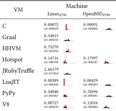
VM Machine

Linux4790 OpenBSD4790

C 0.00075

±0.000029 ±00..00091000002

Graal 0.34815

±0.000233

HHVM 0.75270

±0.002056

Hotspot 0.14716

±0.000708

0.17997

±0.000247

JRubyTruffle 2.66179

±0.011864

LuaJIT 0.00389

±0.000442

0.00429

±0.000003

PyPy 0.44040

±0.001067

0.78696

±0.000481

V8 0.08727

±0.000239

0.12016

[image:17.486.252.438.84.262.2]

±0.000084

[image:17.486.51.232.88.256.2]

Fig. 8. An example where performance changes do not appear to correlate with compilation or GC.

Table 3. VM startup time (in seconds with 99% confi-dence intervals).

it tends to be accompanied by frequent migration between cores. However, it can often be seen that several cores are active during the first few in-process iterations whilst JIT compilation occurs.

5.2 The Effects of Compilation and GC

The large number of non-warmup cases in our data led us to make the following hypothesis:

H3 Non-warmup process executions are largely due to JIT compilation or GC events.

To test this hypothesis, we made use of the debug facilities of HotSpot and PyPy to record the time spent performing JIT compilation and GC. Since recording this additional data could potentially change the results we collect, it is only collected when Krun is explicitly set to ‘instrumentation mode’. This allows us to identify interesting correlations (though we make no claim that they

prove causation). For example, Figure6shows an example where slowdown is clearly correlated

to garbage collection. Similarly, in Figure7, there is a clear correlation between a JIT compilation

and a slowdown. However, in many cases such as Figure8neither JIT compilation, nor garbage

collection, are sufficient to explain odd behaviours.

The relatively few results we have with GC and JIT compilation events, and the lack of a clear message from them, means that we feel unable to validate or invalidate Hypothesis H3. Whilst some non-warmups are plausibly explained by GC or JIT compilation events, many are not, at least on HotSpot and PyPy. When there is no clear correlation, we have very little idea of a likely cause of the unexpected behaviour. It may be that obtaining similar data from other VMs will clarify this issue, but not all VMs support this feature and, in our experience, those that do support it do not always document it accurately.

6 STARTUP TIME

The data presented thus far in the paper has all been collected after the VM has started executing the user program. The period between a VM being invoked and it executing the first line of the

user program is the VM’sstartuptime, and is an important part of a VM’s real-world performance.

(18)

the VM itself; and, for each language under investigation, we provide a ‘dummy’ iterations runner which simply prints out wall-clock time. In other words, we measure the time just before the VM is loaded and at the first point that a user-level program can execute code on the VM; the delta between the two is the startup time. For each VM we run 200 process executions (for startup, in-process iterations are irrelevant, as the user-level program completes as soon as it has printed out wall-clock time).

Table3summarises our startup results. Since Krun reboots before each process execution, these

are measures of a ‘cold’ start and thus partly reflect disk speed etc. (though our machines load VMs from an SSD). As this data clearly shows, startup time varies significantly amongst VMs: taking C

on Linux as a baseline, the fastest VM (LuaJIT) is 5×slower, whilst the slowest VM (JRuby+Truffle)

is around 3500×slower, to startup.

7 THREATS TO VALIDITY

While we have designed our experiment as carefully as possible, we do not pretend to have controlled every possibly confounding variable. It is inevitable that there are further confounding variables that we are not aware of, which may have coloured our results.

We have tried to gain an understanding of the effects of different hardware on benchmarks by using machines with the same OS but different hardware. More distinct hardware (e.g. a non-x86 architecture) is likely to uncover further hardware-related differences. However, hardware cannot be varied in isolation from software: the greater the differences in hardware, the more likely that JIT compilers are to use different components (e.g. different code generators). Put another way, an apples-to-apples comparison across very different hardware is often impossible, because the ‘same’ software is itself different.

We have not systematically tested whether rebuilding VMs affects warmup, an effect noted by Kalibera and Jones, though which seems to have little effect on the performance of JIT compiled

code [Barrett et al. 2015]. However, since measuring warmup largely involves measuring code that

was not created by a JIT compiler, it is possible that these effects may affect our experiment. To a limited extent, the rebuilding of VMs that occurred on each of our benchmarking machines gives some small evidence as to this effect, or lack thereof.

The checksums we added to benchmarks ensure that, at a user-visible level, each benchmark performs equivalent work in each language variant. However, it is impossible to say whether each performs equivalent work at the lowest level or not. For example, choosing to use a different data type in a language’s core library may substantially impact performance. There is also the perennial problem as to the degree to which an implementation of a benchmark should respect other language’s implementations or be idiomatic (the latter being likely to run faster). From our perspective, this is somewhat less important, since we are interested in the warmup patterns of reasonable programs, whether they are the fastest possible or not. It is however possible that by inserting checksums we have created unrepresentative benchmarks, though this complaint could arguably be directed at the unmodified benchmarks too.

Although we have minimised the number of system calls that our in-process iterations runners

make, we cannot escape them entirely. For example, on both Linux and OpenBSDclock_gettime

(which we use to obtain monotonic wall-clock time) contains what is effectively a spin-lock, meaning that there is no guarantee that it returns within a fixed bound. Fortunately, in practise,

clock_gettimereturns far quicker than the granularity of any of our benchmarks. The situa-tion on Linux is complicated by our reading of core-cycle, APERF, and MPERF counters via MSR

device nodes: we calllseekandreadbetween each in-process iteration (we keep the files open

across all in-process iterations to reduce the open/close overhead). These calls are more involved thanclock_gettime: as well as the file system overhead, reading from a MSR device node

(19)

triggers inter-processor interrupts to schedule anRDMSRinstruction on the desired core (causing the running core to save its registers etc.). We are not aware of a practical way to lower these costs.

Although Krun does as much to control CPU clock speed as possible, modern CPUs do not always respect operating system requests. On Linux, we use the APERF/MPERF ratio to check for frequency changes. Although the hoped-for ratio is precisely 1, there is often noticeable variation around this value due to the cost of reading these counters. On active cores the error is small (around 1% in our experience), but on idle cores (which are rarely truly idle, as occasional computation happens on them) it can be relatively high (10% or more is not uncommon; in artificially extreme cases, we have observed up to 200%). We first need to exclude idle cores from any checks. Formally the rate at

which APERF increments is undefined [Intel 2017]. In practise, however, our machines increment

APERF on a fully utilised core at the CPU base frequency (e.g. Linux4790’s CPU increments APERF

at 3.6GHz). We therefore define an idle core to be one whose APERF is 1000×less than this (per

second). We then need to determine a sensible tolerance around the ideal APERF/MPERF ratio of 1, taking into account the error introduced by reading these counters. For the 4790 processor, the frequency values either side of its 3.6GHz base are 3.4GHz and 3.8GHz, which would lead to a 5% difference in the APERF/MPERF ratio (for the 3.5GHz E3-1240 processor, the values either side are 3.3GHz and 3.9GHz i.e. at least a 6% difference in the APERF/MPERF ratio). Based on this,

we define the safe APERF / MPERF ratio to be 1±0.03.5_{We then wrote a simple tool to examine}

every process execution on Linux4790and Linux1240v5, checking that every active core had a safe

APERF/MPERF ratio. Of the 5,520,000 in-process iterations on these two machines, 225 (0.004%)

spread over 10 process executions failed this check, all but 2 on Linux1240v5. Fortunately, outlier detection is designed to deal with such aberrations, and 216 (98%) of these in-process iterations are detected as outliers. Since outliers do not affect changepoint analysis or the statistics we produced, 8 of the 10 process executions are not affected in practise. Since the 2 in-process iterations on

Linux4790do not have noticeably different wall-clock times than their neighbours, and both have an

APERF/MPERF ratio of 1.031 (only marginally above our safe threshold), we do not consider them problematic. The remaining 7 in-process iterations which are not detected as outliers are contained

in 1 process execution of Graal runningfasta: manual inspection shows that these in-process

iterations are fairly evenly spread over the (somewhat noisy) process execution and that two of them led to a small changepoint segment that causes the process execution to be classified as no

steady state rather than warmup. As this⟨VM, benchmark⟩pair was (29 , 1 ), it is likely that if

the processor had run at full speed, the overall benchmark would have been classified as warmup

(as indeed it was on Linux4790). However, overall, the similar figures for Linux4790and Linux1240v5

shown in Table1are strong evidence of the limited effect this is likely to have had on our results.

Our experiments allow the kernel to run on the same core as benchmarking code. We exper-imented extensively with CPU pinning, but eventually abandoned it. After being confused by

the behaviour of Linux’sisolcpusmechanism (whose semantics changes between a normal

and a real-time kernel), we used CPU shielding (cset shield) to pin the benchmarks to the 3

non-boot cores on our machines. However, we then observed notably worse performance for VMs such as HotSpot. We suspect this is because such VMs query the OS for the number of available cores and create a matching number of compilation threads; by reducing the number of available cores, we accidentally forced two of these threads to compete for a single core’s resources.

Address Space Layout Randomisation (ASLR) is, from a performance perspective, a controversial feature. It clearly introduces significant non-determinism into benchmarking, and it is thus tempting