warwick.ac.uk/lib-publications
Original citation:
Advani, Arun and Malde, Bansi. (2018) Methods to identify linear network models : a review.
Swiss Journal of Economics and Statistics, 154 (12).
Permanent WRAP URL:
http://wrap.warwick.ac.uk/97307
Copyright and reuse:
The Warwick Research Archive Portal (WRAP) makes this work of researchers of the
University of Warwick available open access under the following conditions.
This article is made available under the Creative Commons Attribution 4.0 International
license (CC BY 4.0) and may be reused according to the conditions of the license. For more
details see:
http://creativecommons.org/licenses/by/4.0/
A note on versions:
The version presented in WRAP is the published version, or, version of record, and may be
cited as it appears here.
O R I G I N A L A R T I C L E
Open Access
Methods to identify linear network
models: a review
Arun Advani
1and Bansi Malde
2*Abstract
In many contexts we may be interested in understanding whether direct connections between agents, such as declared friendships in a classroom or family links in a rural village, affect their outcomes. In this paper, we review the literature studying econometric methods for the analysis of linear models ofsocial effects, a class that includes the ‘linear-in-means’ local average model, the local aggregate model, and models where network statistics affect outcomes. We provide an overview of the underlying theoretical models, before discussing conditions for identification using observational and experimental/quasi-experimental data.
Keywords: Networks, Social effects, Peer effects, Econometrics
JEL Classification: C31, C81, Z13
Background
Researchers and policymakers are often interested in identifying whether and the extent to which direct con-nections between agents affect their outcomes. For exam-ple, does the schooling performance of an individual depend on that of her friends? Does the health seeking behaviour of one’s relatives influence one’s own health seeking behaviour? Are firms’ investment and pay deci-sions influenced by the behaviour of firms in the same or closely-related industry? The identification and estima-tion of such social or network effects—direct spillovers from the characteristics or outcomes of one agent to the outcome of others—is of central interest in empirical research on networks in economics.
This paper reviews recent developments in methods to identify linear peer effect models using networks data— data with detailed information on the exact interactions between agents—when a single cross section of data is available. Linear models are the most widely used in empirical work, with many econometric methods devel-oped to work with these, making them a natural choice to consider in this review1. Moreover, panel data on the net-work have until recently only rarely been available, so the majority of methods focus on the case with a single cross section of data2.
*Correspondence:[email protected]
2University of Kent, Canterbury and Institute for Fiscal Studies, London, UK Full list of author information is available at the end of the article
We provide an overview of a number of commonly used empirical specifications, the underlying theoretical models that generate them; and the conditions for the causal identification of parameters with cross-sectional data. We first consider three ‘local’ models, where only an agent’s direct connections (orneighbours) affect his out-come. The three specifications allow this effect to depend on the average outcome, total outcome, or both, of his neighbours. In the absence of information on interactions within a network (or group), identification of social effect parameters is greatly complicated by the so-called reflec-tion problem, a form of simultaneity where it is not pos-sible to identify who influences whom within the network or reference group (Manski 1993). Information on the exact interactions within a network can break this simul-taneity for a wide range of network structures, allowing for identification of social effect parameters3.
Recent theoretical analyses have shown that the struc-ture of networks, as well as positions of agents within them influences agents’ overall outcomes on dimensions such as information diffusion and risk sharing, among others (Bloch et al. 2008; Jackson et al. 2012; Banerjee et al.2013). The availability of detailed network data has motivated the testing of implications of these models in recent work. We thus next discuss models where the entire structure of the network might matter for an indi-vidual’s outcome. Finally, we discuss how experimental
and quasi-experimental variation could be used to provide additional variation to uncover social effects.
Our objective is to provide an overview of methods developed under the assumption that the network is (conditionally) exogenously formed: that is, there are no unobserved individual variables within the network that determine who links with whom. This is an important issue that is the subject of much recent research. A com-panion paper (Advani and Malde2016), as well as other recent reviews (e.g. Graham 2015; Chandrasekhar2015; de Paula 2016), provide overviews of this issue and of possible methods to deal with this.
An important issue in the practical estimation of social effects relates to the definition and measurement of the network. Our review proceeds assuming that the researcher perfectly observes and measures the network (or network neighbours) relevant for the outcome(s) of interest. Clearly, the researcher’s choice of network to use will influence the estimated parameters and poten-tially lead to different policy implications. However, few existing datasets collect information on more than one type of network, so that in practice, researchers are often restricted in their definition of the network by the avail-able data. Nonetheless, existing studies indicate that the definition of the network is important. For example, Sacerdote (2001) finds that only students’ individual room-mates affect their college performance, while a broader set of peers matters for decisions related to social group participation; Renna et al. (2008) document that adolescents’ weights are more responsive to those of their friends of the same gender, while Patacchini et al. (2016) find that adolescent friendships lasting longer than 1 year have persistent effects on adolescents’ education outcomes, while shorter-lived friendships do not. Mea-surement error on the network will also bias parameter estimates. A more detailed overview of this issue, as well as of methods to deal with it, is provided in Advani and Malde (2014) and another companion paper (Advani and Malde2016).
To illustrate the practical restrictions imposed by each of the different models, empirical specifications and con-ditions for causal identification, we will use a simple and widely studied question in the education and labour eco-nomics literatures: How is a teenager’s schooling perfor-mance influenced by his friends? This is also a question of great policy interest.4More specifically, this paper will provide an overview of methods that can yield answers to questions such as ‘Is a teenager’s schooling perfor-mance influenced by the average schooling perforperfor-mance of her friends?’; ‘Do teenagers gain more utility from studying if their friends also study?’; ‘What is the rel-ative importance of the average schooling performance of a teenager’s friends, and of complementarities aris-ing from one’s friends’ studyaris-ing decisions in shaparis-ing a
teenager’s overall schooling performance?’; and ‘How does a student’s popularity influence his/her schooling perfor-mance?’ The same methods can also be applied to answer analogous questions about interactions between many other types of agents.
The literature on methods for networks data is broad and developing rapidly. We therefore focus our review on the issues outlined above, leaving aside a number of other interesting areas, including methods to deal with endogenous network formation and measurement error in the network, which we survey elsewhere (Advani and Malde 2016). In addition, though many of the methods reviewed here either build on or apply methods developed in spatial econometrics, it is not our objective to provide an overview of spatial econometric methods (see instead Anselin1988). Boucher and Fortin (2015) provide a com-plementary review, though they do not cover methods using experimental and quasi-experimental variation.
The rest of the paper is organised as follows. The “Notation” section outlines the notation used in this paper. The “Local average models” section provides an overview of the local average model, where the average of neighbours’ outcomes is allowed to affect an individual’s outcome. In the “Local aggregate model” section, we cover the local aggregate model, where instead it is the total of neighbours’ outcomes that matters. In the “Hybrid local models” section, we consider hybrid local models, which allow both local average and local aggregate type effects. We consider models including network statistics that are not purely local, in the “Models with network characte-ristics” section. Finally, we show how experimental and quasi-experimental variation can be used to identify social effects in the “Experimental variation” section, before concluding.
Notation
We begin by outlining the notation we use throughout the paper. We define anetworkorgraph g = (Ng,Eg)as a set of nodes,Ng, and edges or links,Eg.5The nodes rep-resent individual agents, and the edges reprep-resent the links between pairs of nodes. In economic applications, nodes are usually individuals, households, firms or countries. Edges could be social ties such as friendship, kinship, or co-working, or economic ties such as purchases, loans, or trade. The number of nodes present ingisNg = |Ng|, and the number of edges is Eg = |Eg|. We define
GN = {g: |Ng| =N}as the set of all possible networks on Nnodes.
In the simplest case—the binary network—any
will be referred to as‘second-degree neighbour’. Typically, it is convenient to assume that ii ∈/ Eg ∀i ∈ Ng. Edges may be directed, so that a link from nodeito nodejis not the same as a link from nodejto nodei; in this case, the network is adirected graph(ordigraph).
Network graphs, whether directed or not, can also be represented by anadjacency matrix,Gg, with typical ele-mentGij,g. This is an Ng ×Ng matrix with the leading diagonal normalised to 0. When the network is binary, Gij,g= 1 ifij ∈ Eg, and 0 otherwise, while for weighted graphs,Gij,g = wei(i,j). We will use the notationGi,g to denote theith row of the adjacency matrixGg, andGi,gto denote itsith column6. Many models defined for binary networks make use of the row-stochastic adjacency matrix or influence matrix, G˜g, whose elements are defined as
˜
Gij,g=Gij,g/jGij,g7.
In what follows, we will frequently work with data from a number of network graphs. Graphs for different net-works will be indexed, in a slight abuse of notation, by g = 1,. . .,M, whereMis the total number of networks in the data. Node-level variables will be indexed withi= 1,. . .,Ng, where Ng is the number of nodes in graphg. Node-level outcomes will be denoted byyi,g, while exoge-nous covariates will be denoted by the 1×K vectorxi,g and common network-level variables will be collected in the 1×Qvector,zg.
The node-level outcomes, covariates and network-level variables can be stacked for each node in a network. In this case, we will denote the stacked Ng × 1 out-come vector as yg and the Ng × K matrix stacking node-level vectors of covariates for graphgasXg. Com-mon network-level variables for graphg will be gathered in the matrix Zg = ιgzg where ιg denotes an Ng × 1 vector of ones. The adjacency and influence matri-ces for network g will be denoted by Gg and G˜g. At times we will also make use of the Ng × Ng identity matrix,Ig, consisting of ones on the leading diagonal, and zeros elsewhere.
Finally, we introduce notation for vectors and matri-ces stacking together the network-level outcome vectors, covariate matrices and adjacency matrices for all net-works in the data.Y = y1,. . .,yM is anMg=1Ng ×1 vector that stacks together the outcome vectors; G =
diag{Gg}gg==1M denotes the Mg=1Ng × Mg=1Ng block-diagonal matrix with network-level adjacency matrices along the leading diagonal and zeros of the diagonal, and analogouslyG˜ = diag{ ˜Gg}gg==1M (with similar dimensions asG) for the influence matrices; andX = X1,. . .,XM
and Z = Z1,. . .,ZM are respectively, Mg=1Ng × K andMg=1Ng×Qmatrices, that stack together the covari-ate matrices across networks. Finally, we define the vec-tor ι as a Mg=1Ng × 1 vector of ones and the matrix
L = diagιggg=1=M, as an Mg=1Ng × M matrix with each column being an indicator for being in a particular network.
Local average models Setup
In local average models, an agent’s outcome (or choice) is influenced by the average outcome of its neighbours8.
Thus, an individual’s schooling effort or performance is influenced by the average schooling effort or perfor-mance of his friends. We characterise the individual as a node, i, in network g, with outcome yi,g. This out-come is modelled as being influenced by the individual’s own observed characteristics,xi,g, scalar unobserved het-erogeneity εi,g, observed network characteristics zg, an unobserved network characteristic νg, and the average outcomes and characteristics of neighbours,Nj=1g G˜ij,gyj,g
and K k=1
Ng j=1 ˜
Gij,gxj,k,g. Below, we consider identification
con-ditions when data are available from multiple networks, though some results apply to data from a single network9. Stacking together data from multiple networks yields the following empirical specification, expressed in matrix terms:
Y =αι+βGY˜ +Xγ + ˜GXδ+Zη+Lν+ε (1)
where Y, ι, G˜, X, Z, L andν are as defined previously. Pre-multiplying the vector Y by G˜ gives a vector con-taining, for each individual, the average outcome of his neighbours, and similarlyGX˜ is a vector of the average characteristics of his friends. The social effect of interest is
β, the effect of an increase in the mean of neighbours’ out-come on the individual’s outout-come. This is often described as the ‘endogenous social effect’, in contrast to the (vector of ) ‘contextual effect(s)’ (or ‘exogenous social effect(s)’),δ, which represent the effect of an increase in neighbours’ characteristics. ν is described as the ‘correlated effect’, capturing the correlation in individuals’ outcomes due to common (unobserved) shocks.
Given the simple empirical form of this model, it has been widely applied in the economics literature. Examples include:
• Understanding how the average schooling
performance of an individual’s peers influences the individual’s own performance in a setting where students share a number of different classes (e.g. De
Giorgi et al.2010), or where students have some (but
not all) common friends (e.g. Bramoullé et al.2009).
• Understanding how non-market links between firms
arising from company directors being members of multiple company boards influence firm choices on
Although this specification is widely used in the empirical literature, few studies consider or acknowledge the form of its underlying economic model, even though parame-ter estimates are subsequently used to evaluate alparame-ternative policies and to make policy recommendations. Indeed, parameters are typically interpreted as in the economet-ric model of Manski (1993), whose parameters do not map back to ‘deep’ structural (i.e. policy invariant) parameters without an economic model.
Theoretical foundations
An economic model that leads to this specification is one where nodes have a desire to conform to the average behaviour and characteristics of their neighbours (Akerlof 1980; Jones1984; Bernheim1994; Patacchini and Zenou 2012). In our schooling example, conformism implies that individuals would want to exert a similar amount of effort in their school work as their friends so as to ‘fit in’. Condi-tional on the individual’s own characteristics which affect his school effort, if his friends exert relatively low effort in their school work, he will reduce his effort. Below we write out this model more formally and demonstrate how it leads to Eq.1.
Conformism is commonly modelled by individual pay-offs that are decreasing in the distance between own outcome and network neighbours’ average outcomes10. Payoffs are also allowed to vary with an individual het-erogeneity parameter, πi,g(Xg,G˜i,g), which captures the individual’s ability or productivity associated with the outcome:
Ui
yi,g;y−i,g,Xg,G˜i,g
= ⎛
⎝πi,gXg,G˜i,g
i,g
−1 2
⎛ ⎝yi,g−2β
Ng
j=1 ˜ Gij,gyj,g
⎞ ⎠ ⎞ ⎠yi,g
(2)
β in Eq.2can be thought of as a taste for conformism. Although we write this model as though individuals are perfectly able to observe each others’ actions, this assump-tion can be relaxed. In particular, an econometric specifi-cation similar to Eq.1can be obtained from a static model with imperfect information (see Blume et al.2015).
The best response function derived from the first order condition with respect toyi,gis:
yi,g=πi,g
Xg,G˜i,g
+β
Ng
j=1
˜
Gij,gyj,g (3)
Patacchini and Zenou (2012) derive the conditions under which a Nash equilibrium exists, and characterise properties of this equilibrium.
Note that this is not the only economic model that leads to an empirical specification of this form: a similar specification arises from, for example, models of perfect risk sharing11. Here, when preferences are homogeneous and risk is perfectly shared, the consumption of risk-averse households will co-move with the average house-hold consumption in the risk sharing group or network Townsend (1994).
The individual heterogeneity parameter, πi,g(Xg,G˜i,g), can be modelled as a linear function of observed and unobserved individual and network characteristics:
πi,g
Xg,G˜i,g
=xi,gγ+ Ng
j=1
˜
Gij,gxj,gδ+zgη+νg+εi,g
(4)
Substituting for this in Eq. 3, we obtain the following best response function for individual outcomes:
yi,g=β Ng
j=1
˜
Gij,gyj,g+xi,gγ+ Ng
j=1
˜
Gij,gxj,gδ+zgη+νg+εi,g
(5)
Then, stacking observations for all nodes in multiple networks, we obtain Eq.1, which can be taken to the data.
Identification
Without network fixed effects
Bramoullé et al. (2009) study the identification and esti-mation of Eq. 1in observational data with detailed net-work information or data from partially overlapping peer groups.12 To proceed further, one needs to make some assumptions on the relationship between the unobserved variables—ν andε—and the other right-hand side vari-ables in Eq.1.
We first consider identification under the assumptions that Eε|X,Z,G˜ = 0 andEν|X,Z,G˜ = 0, i.e. both the individual level error term,ε and the network level unobservable are assumed to be mean independent of the observed individual and network-level characteristics and of the network. We will later relax the assumption onν.
Under these assumptions, the parameters{α,β,γ,δ,η} are identified if
I,G˜, G˜2
are linearly independent. Iden-tification thus relies on the network structure. In particu-lar, the condition would not hold in networks composed only of cliques—subnetworks comprising of completely connected components—of the same size, and where the diagonal terms in the influence matrix,G˜ are not set to 0. In this case,G˜2can be expressed as a linear function of
In an undirected network (such as that in the left panel in Fig.1below), this identification condition holds when there exists a triple of nodes(i,j,k)such thatiis connected to j but not k, and j is connected to k. The exogenous characteristics of k, xk,g, directly affect j’s outcome, but not (directly) that of i, hence forming valid instruments for the outcome of i’s neighbours (i.e. j’s outcome) in the equation for nodei. Intuitively, this method uses the characteristics of second-degree neighbours who are not direct neighbours as instruments for outcomes of direct neighbours.
It is thus immediately apparent why identification fails in networks composed only of cliques: in such networks, there is no triple of nodes(i, j, k)such thatiis connected toj, andjis connected tok, butiis not connected tok.
In the directed network case, the condition is some-what weaker, requiring only the presence of an intransitive triad: that is, a triple such thatij∈E,jk∈ E andik ∈/ E (as in the right panel of Fig. 1 above).13 This is weaker than in undirected networks, which would also require thatki∈/E.
These conditions impose strong restrictions on behaviour. The identification condition for undirected networks, for example, relies on i and k not influenc-ing one another directly, which might be too strong an assumption in contexts such as within-classroom networks, where it is not unreasonable to assume that all students are likely to interact with one another, and hence influence one another. Similarly, the identification assumption in a directed network is likely to hold in spe-cific contexts only: for example, the effort of check-out workers who face the same direction (or are arranged in a circle) would be influenced by that of the colleagues that they can see, satisfying the identification condition (Mas and Moretti2009).
Let us consider how this method could be applied to identify the influence of the average schooling perfor-mance of an individual’s friends on the individual. Poten-tial variables that one might include as controls include the individual’s age, gender, and parental income; the aver-age aver-age, gender, and parental income of his friends; and some observed school characteristics such as expenditure per pupil. Assume first that the underlying friendship net-work in this school is undirected as in the left panel of Fig.1, so that ificonsidersjto be his friend,jalso consid-ersito be his friend.jalso has a friendkwho is not friends withi. We could then use the age, gender, and parental
income ofkas instruments for the schooling performance of j in the equation for i. If instead, the network were directed as in the right panel of Fig.1, where the arrows indicate who is affected by whom (i.e.iis affected byjin the Figure, and so on), we can still use the age, gender, and parental income ofkas instruments for the school perfor-mance ofjin the equation forieven thoughkis connected withi. This is possible since the direction of the relation-ship is such thatk’s school performance is affected byi’s performance, but the converse is not true.
Including network fixed effects
The identification result above requires that the network-level unobservable term be mean independent of the observed covariates, X and Z, and of the network, G˜. However, in many circumstances, one might be concerned that unobservable characteristics of the network might be correlated with X, so thatEν|X,Z,G˜ = 0. In the schooling context, where the network of interest is often constrained to be within the same school, a large literature (e.g. Black1999; Gibbons and Machin2003; Bayer et al. 2007) indicates that wealthier parents choose to live in areas with good schools, making it likely that children with higher parental income will be in schools with teachers who have better unobserved teaching abilities. A natural solution is to include network fixed effects,Lν˜, which will control for the network-level unobservable,Lν, though at the cost of allowing us to identifyη.
Since the fixed effects themselves are generally not of interest, to ease estimation they are removed using a within transformation. This is done by pre-multiplying Eq.1byJ, a block diagonal matrix that stacks the network-level transformation matricesJg = Ig − N1g
ιgιg
along the leading diagonal, and off-diagonal terms are set to zero. This subtracts the network-level mean of the out-come, giving a vectorJYof deviations from the mean. The resulting model is of the following form:
JY =βJGY˜ +JXγ +JGX˜ δ+Jε (6)
The identification condition here imposes a stronger requirement on network structure: now, the matrices
I, G˜,G˜2, G˜3
need to be linearly independent. This requires that there exists a pair of agents(i,l)such that the shortest path between them is of length 3. That is,iwould need to go through at least two other nodes to get tol(as in Fig.2below). The presence of at least two intermediate
a
b
[image:6.595.56.540.660.723.2]agents allows the researcher to use the characteristics of third-degree neighbours (of-of-neighbours who are not direct (of-of-neighbours or (of-of- neighbours-of-neighbours) as an additional instrument to account for the network fixed effect.
A concern that arises when applying this method is that of instrument strength. Bramoullé et al. (2009) find that this varies with graph density, i.e. the pro-portion of node pairs that are linked; and the level of clustering, i.e. the proportion of node triples such that precisely two of the possible three edges are connected.14 Instrument strength is declining in den-sity, since the number of intransitive triads tends to zero, reducing the variation in the instrument. The results for clustering are non-monotone and depend on density.
The discussion thus far has assumed that the network through which the endogenous social effect operates is the same as the network through which the contextual effect operates. It is possible to allow for these two net-works to be distinct. This could be useful in the school setting, for instance, where contextual effects could be driven by the average characteristics of all students in the school, while endogenous effects by the outcomes of a subset of students who are friends. Such a formulation allows for a more flexible representation of the environ-ment: the contextual effect could operate through, for example, the resources available to a school, which might depend on the parental income of all students (if schools are financed through local taxation), while peer influ-ences on effort or performance might come only from friends.
Let GX,g andGy,g denote the network-level adjacency matrices through which, respectively, the contextual and endogenous effects operate. As before, we define the block diagonal matrices GX = diag
GX,g g=M
g=1 and Gy =
diagGy,g g=M
g=1 . Blume et al. (2015) study identification of this model assuming that both networks are (condition-ally) exogenous and show that when the matricesGyand
GX are observed by the econometrician, and at least one ofδandγ is non-zero, then the necessary and sufficient conditions for the parameters of Eq. 1 to be identified
are that the matrices I, Gy, GX andGyGX are linearly independent.
Local aggregate model
The local aggregate class of models, studied theoretically by Ballester et al. (2006), Calvó-Armengol et al. (2009), and Bramoullé et al. (2014), and empirically by Calvó-Armengol et al. (2009), Lee and Liu (2010), and Liu et al. (2012), considers settings where agents’ utilities are a function of the aggregate outcomes (or choices) of their neighbours. This is in contrast with local average models, where utilities are a function of the difference between own outcome and the average outcome of one’s neighbours. The local aggregate model thus encompasses a different assumption on behaviour—it applies to sit-uations where there are strategic complementarities or strategic substitutabilities—and allows dyad-level social effects to aggregate at a network or group level.
Examples of cases where strategic complementarities and substitutabilities are likely to be at play and thus where a local aggregate, rather than local average model, would be more appropriate include:
• An individual’s costs of engaging in crime may be
lower when his neighbours also engage in crime (e.g. Bramoullé et al.2014).15
• An agent is more likely to learn about a new product
and how it works if more of his neighbours know about it and have used it.
• A student gains more utility from undertaking effort
in studying if his friends also undertake more effort
(e.g. Calvó-Armengol et al.2009).
Setup and theoretical foundations
The local aggregate model corresponds to the following empirical specification:
Y=αι+βGY+Xγ +GX˜ δ+Zη+Lν+ε (7)
where Y, G,X andZ are as defined earlier. In contrast to the local average model, G˜ has been replaced by G. As before, the social effect of interest is β, which now represents the effect of the aggregate outcome of one’s neighbours on one’s own outcome.
[image:7.595.61.540.617.700.2]This specification can be motivated by the best responses of a game in which nodes have linear-quadratic utility and there are strategic complementarities or sub-stitutabilities between the actions of a node and those of its neighbours. A model of this type has been stud-ied by among others, Ballester et al. (2006) and Bramoullé et al. (2014). The former focus on the case of strategic complementarities, while the latter study the case with strategic substitutabilities and characterise all equilibria of this game. In this model, the utility function for agentiin networkgtakes the following form:
Ui
yi,g;y−i,g,Xg,Gg
= ⎛
⎝πi,gXg,G˜i,g
− 1 2
⎛ ⎝yi,g −2β
Ng
j=1
Gij,gyj,g ⎞ ⎠ ⎞ ⎠yi,g
(8)
where yi,g is i’s action or choice, and πi,g(Xg,G˜i,g) is, as before, an individual heterogeneity parameter16. This has the same form as Eq. 2, but with G replacing G˜.
πi,g(Xg,G˜i,g)is again typically parameterised as:
πi,g
Xg,G˜i,g
=xi,gδ+ n
j=1 ˜
Gij,gxj,gγ +zgη+νg+εi,g
so that individual heterogeneity is a function of a node’s own characteristics, the average characteristics of its neighbours, network-level observed characteristics, and some unobserved network- and individual-level terms. This model shares some features with the model of Blume et al. (2015), as different network matrices are used to capture the effects of neighbours’ outcomes and charac-teristics, which helps to ease identification.
The quadratic cost of own actions means that in the absence of any network, there would be a unique opti-mal amount of effort the node would exert, as in the local average model.β >0 implies that neighbours’ actions are complementary to a node’s own actions, so that the node increases his actions in response to those of his neigh-bours. Ifβ < 0, then nodes’ actions are substitutes, and the reverse is true. Nodes chooseyi,g so as to maximise their utility.
The best response function is:
y∗i,gGg
=β n
j=1
Gij,gyj,g+xi,gδ+ n
j=1
˜
Gij,gxj,gγ+zgη+νg+εi,g
(9)
Ballester et al. (2006) solve for the Nash equilibrium of this game whenβ >0 and show that when|βωmax(Gg)|<1, where ωmax(Gg) is the largest eigenvalue of the matrix
Gg, the equilibrium is unique and the equilibrium out-come relates to a node’s Katz-Bonacich centrality, which is defined asb(Gg,β)=(Ig−βGg)−1(ιg)17,18.
Bramoullé et al. (2014) study the game with strategic substitutabilities between the action of a node and those of its neighbours. In this case, when one agent chooses one action, his neighbours would choose the opposite action, inducing their neighbours to choose a similar action to the first agent, and so on. In equilibrium, the agent’s choice is influenced by the direct choice of his neighbours, as well as by the aggregated sum of these opposing choices across different network paths. Bramoullé et al. (2014) charac-terise the set of Nash equilibria of the game and show that they depend on the lowest eigenvalue of the network adja-cency matrix,ωmin(Gg). This eigenvalue is negative and relates to the aggregated effect of agents’ choices on oth-ers. When it is large in magnitude, the opposing forces outlined above could go in many different directions, lead-ing to multiple equilibria. When it is sufficiently small, i.e. β|ωmin(Gg)| < 1, a unique equilibrium exists since the opposing forces ‘balance out’ to converge to a single point. When multiple equilibria are possible, they must be accounted for in any empirical analysis. Methods devel-oped in the literature on the econometrics of games may be applied here (Bisin et al.2011). See de Paula (2013) for an overview. Below, we focus on conditions under which the social effect parameter is identified when a unique equilibrium exists.
When a unique equilibrium exists, this theoretical setup implies the following empirical model (stacking data from multiple networks):
Y =αι+βGY+Xγ + ˜GXδ+Zη+Lν+ε (10)
where variables and parameters are as defined above.
Identification
Identification of Eq.10using observational data has been studied by Calvó-Armengol et al. (2009), Lee and Liu (2010) and Liu et al. (2012). They proceed under the assumption thatEε|X,Z,G,G˜=0 andEν|X,Z,G,G˜=
0. That is, the node-varying error component is condi-tionally mean independent of node- and network-level observables and of the network, while the network-level unobservable could be correlated with node- and network-level characteristics and/or the network itself.
unobservable factors that determine the choice of network or link formation within the chosen network.
To proceed, we assume that data are available for mul-tiple networks. Then, as in the “Local average models” section, we replace the network-level observables,Z, and the network-level unobservable,Lνin Eq.10with network fixed effects,Lν˜, whereν˜is aM×1 vector that captures the network fixed effects.
To account for the fixed effect, a within-transformation is applied, as in the “Local average models” section. This transformation is represented by the block diagonal matrixJ that stacks the following network-level transfor-mation matrices—Jg = Ig− N1g
ιgιg
—along the leading diagonal, with off-diagonal terms set to 0. The resulting model, analogous to Eq.6, is:
JY =βJGY+JXγ +JGX˜ δ+Jε (11)
The model above suffers from the reflection problem, sinceY appears on both sides of the equation. However, the parameters of Eq. 11 can be identified using linear instrumental variables (IV) if the deterministic part of the right-hand side, [E(JGY),JX,JGX˜ ], has full column rank. To see the conditions under which this is satisfied, we examine the term with the endogenous variable,E(JGY). Under the assumption that|βωmax(Gg)| < 1, we obtain the following from the reduced form equation of Eq.10:
E(JGY)=JGX+βG2X+. . .γ+JGGX˜ +βG2GX˜ +. . .δ
+JGL+βG2L+. . .ν˜
(12)
We can thus see that if the matrices {I,G,G˜,GG˜} are linearly independent, andγ,δ, andν˜each have some non-zero terms, the parameters of Eq.10are identified19. Node degree (GL), along with the sum of the exogenous charac-teristics of the node’s direct neighbours (GX), and sum of the average exogenous characteristics of its second-degree neighbours (GGX˜ ) can be used as instruments for the total outcome of the node’s neighbours (GY). That node degree can be used as an instrument follows intuitively from the theoretical model: when there are dyad-level strategic complementarities, an individual’s own outcome will be a weakly increasing function of the number of his direct neighbours. Moreover, the availability of node degree as an instrument can allow one to identify parameters with-out using the exogenous characteristics,X, of second- or higher-degree network neighbours, which can be particu-larly advantageous when only sampled data are available, as shown by Liu (2013).
In terms of practical application, consider using this method to identify whether there are complementarities between the schooling performance of an individual and that of his friends, conditional on his own characteristics (age, gender, and parental income), the composition of his
friends (average age, gender, and parental income), and some school characteristics. Then, if there are individu-als in the same network with different numbers of friends, and the matrices I,G,G˜,GG˜are linearly independent, the individual’s degree, along with the total characteristics of his friends (i.e. total age, gender, and parental income) and the sum of the average age, gender, and parental income of the individual’s friends of friends can be used as instruments for the sum of the individual’s friends’ school-ing performance. Similar to the local average model, this strategy relies on a researcher being able to define rea-sonably well direct, as well as indirect, neighbours, which might be less clear in some contexts.
Parameters can still be identified if there is no varia-tion in node degree within a network for all networks in the data, but there is variation in degree across networks. In this case,Gg = ¯dgG˜g and
E(JGY),JX,JGX˜ has full column rank if the matrices I,G,G˜,GG˜,G˜2,GG˜2 are linearly independent and γ and δ each have non-zero terms20. This requires the presence of some pair of nodes iandk, who are only indirectly connected. Finally, when there is no variation in node degree within and across all networks in the data, parameters can be identified using a similar condition as encountered in the “Local average model” section above: the matricesI,G˜,G˜2,G˜3should be linearly independent.
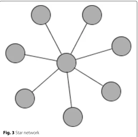
It is possible to identify model parameters in the local aggregate model in networks where the local average model parameters cannot be identified. For example, in a star network (see Fig.3), there is no pair of agents that has a geodesic distance (i.e. shortest path) of three or more, so this fails the identification condition for the local
[image:9.595.305.540.494.728.2]average model with fixed effects. However, there is varia-tion in node degree within the network and the matrices
Ig,Gg,G˜g,GgG˜gcan be shown to be linearly independent, thus satisfying the identification conditions for the local aggregate model.
Hybrid local models
The local average and local aggregate models embody dis-tinct mechanisms through which social effects arise. One may be interested in jointly testing these mechanisms, and empirically identifying the most relevant one for a par-ticular context. Liu et al. (2014a) present a framework nesting both the local aggregate and local average models, allowing for this.
Setup and theoretical foundations
The utility function for nodeiin networkgthat nests both the (linear) local aggregate and local average models has the following form:
Ui
yi,g;y−i,g,Xg,G˜i,g,Gi,g
=
⎛
⎝πi,gXg,G˜i,g
+β1
Ng
j=1
Gij,gyj,g
−1
2
⎛ ⎝yi,g−2β2
Ng
j=1
˜
Gij,gyj,g
⎞ ⎠ ⎞ ⎠yi,g
(13)
whereπi,g(Xg,G˜i,g)is node-specific observed heterogene-ity, which affects the node’s marginal return from the chosen outcome levelyi,g. A node’s utility is thus affected by the choices of its neighbours through changing the marginal returns of its own choice (e.g. in a schooling con-text, an individual’s studying effort is more productive if his friends also study), as in the local aggregate model, and by a cost of deviating from the average choice of its neigh-bours (i.e. individuals face a utility cost if they study when their friends do not study), as in the local average model.
The best reply function for a node i nests both the local average and local aggregate terms. Liu et al. (2014a) prove that under the condition thatβ1 ≥ 0,β2 ≥ 0 and
dmax
g β1+β2<1, wheredgmaxis the largest degree in net-workg, the simultaneous move game has a unique interior Nash equilibrium in pure strategies. Note that this rules out the possibility of individuals’ actions being strategic substitutes (i.e.β < 0), as for example if one student in a group needs to supply effort on homework so that the others can copy him.
The econometric model, assuming that the node-specific observed heterogeneity parameter takes the form
πi,g
Xg,G˜i,g
=xi,gγ +Nj=1g G˜ij,gxj,gδ+zgηg+νg+εi,g, is as follows:
Y =αι+β1GY+β2GY˜ +Xγ+ ˜GXδ+Zη+Lν+ε (14)
using the same notation as before.
With data from only a single network it is not possible to separately identifyβ1 andβ2and hence test between
the local aggregate and local average models (or indeed find that the truth is a hybrid of the two effects). Iden-tification of parameters is considered when data from multiple networks are available under the assumption that Eεi,g|Xg,Zg,Gg,G˜g
= 0 andEνg|Xg,Zg,Gg,G˜g
= 0. Thus, as in the “Local average models” and “Local aggre-gate model” sections above, the individual error term,
εi,g is assumed to be mean independent of node- and network-level observable characteristics and the network. The network-level unobservable,νg, by contrast is allowed to be correlated with node- and network-level character-istics and/or the network.
Identification
To proceed, as in the local average and local aggre-gate model,Zη andLν are replaced by a network-level fixed effect,Lν˜, which is then removed using the within-transformation, J. The resulting transformed network model is:
JY =β1JGY+β2JGY˜ +JXγ +JGX˜ δ+Jε (15)
When there is variation in the degree within a networkg, the reduced form equation of Eq. 15implies that JG(I− β1G−β2G˜)−1L can be used as an
instru-ment for the local aggregate termJGY andJG˜(I−β1G− β2G˜)−1L can be used as an instrument for the local
average termJGY˜ . The model parameters may in prin-ciple thus be identified even if there are no node-level exogenous characteristics, X, in the model, as long as
β1 = 0. However, ifβ1 = 0, the model excluding
exoge-nous characteristics,X, is tautological—in this case one is simply regressing individuals’ outcomes on the mean of the outcomes (see Angrist 2014, for further discus-sion). The availability of such characteristics offers more possible IVs: in particular, the total and average exoge-nous characteristics of direct and indirect neighbours can be used as instruments. These are necessary for identi-fication when all nodes within a network have the same degree, though average degree may vary across networks. In this case, parameters can be identified if the matrices
I,G,G˜,GG˜,G˜2,GG˜2,G˜3are linearly independent21. If, however, all nodes in all networks have the same degree, it is not possible to identify separately the parametersβ1
andβ2.
should have no additional explanatory power in the orig-inal model, i.e. its coefficient should not be significantly different from zero. Thus, to identify which of the local average or local aggregate mechanisms is more relevant for a specific outcome, one could first estimate one of the models (e.g. the local average model), and obtain the predicted outcome value under this mechanism. In a sec-ond step, estimate the other model (in our example, the local aggregate model) and include as a regressor the pre-dicted value from the other (i.e. local average) model. If the mechanism underlying the local average model is also relevant for the outcome, the coefficient on the predicted value will be statistically different from 0. The converse can also be done to test the relevance of the second model (the local aggregate model in our case) (see Liu et al. (2014a) for more details).
Models with network characteristics
The models considered thus far allow for a node’s out-comes to be influenced only by outout-comes of its neigh-bours, so-called local models. However, the broader net-work structure may affect node- and aggregate netnet-work- network-outcomes through more general functionals or features of the network. Depending on the theoretical model used, there are different predictions on which network features relate to different outcomes of interest. For example, the DeGroot (1974) model of social learning implies that a node’s eigenvector centrality, which measures its ‘impor-tance’ in the network by how important its neighbours are, determines how influential it is in affecting the beliefs of other nodes.
Empirical testing and verification of the predictions of these theoretical models has greatly lagged the theoretical literature due to a lack of datasets with both information on network structure and socio-economic outcomes of interest. The recent availability of detailed network data from many contexts has begun to relax this constraint.
The following types of specification are typically esti-mated when assessing how outcomes vary with network structure, for node-level outcomes:
Y=fy(wy(G,Y),X,wx(G,X),Z)+ε (16)
and network-level outcomes: ¯
Y=fy¯(w¯y¯(G),X¯,w¯x¯(G,X¯))+u (17)
fy(.)andf¯y(.)are functions that specify the shape of the relationship between the network statistics and the node-and network-level outcomes. Though, in principle, the shape offy(.)should be guided by theory (where possi-ble), through the rest of this section, we takefy(.)to be a linear index in its argument, as is common in the liter-ature.wy(G,Y)is anMg=1Ng×R
matrix stacking the
(1×R) node-level vector of network statistics that vary
at the node or network level and that may be interacted with Y22. w¯y¯(G)is an(M× ¯R) matrix containing theR¯
network statistics in the network-level regression.X is a matrix of observable characteristics of nodes,wx(G,X) interacts network statistics with exogenous characteris-tics of nodes, andZandX¯ are network-level observable characteristics.w¯x¯(G,X¯)interacts network statistics with
network-level observable characteristics.
The complexity of networks poses an important chal-lenge in understanding how outcomes vary with network structure. In particular, there are no sufficient statistics that fully describe the structure of a network. For example, networks with the same average degree may vary greatly on dimensions such as density, clustering and average path length among others. Moreover, the adjacency matrix,G, which describes fully the structure of a network, is too high-dimensional an object to include directly in tests of the influence of broader features of network structure. Theory can provide guidance on which statistics are likely to be relevant, and also on the shape of the relationship between the network statistic and the outcome of inter-est. A limitation though is that theoretical results may not be available (given currently known techniques) for out-comes one is interested in studying. This is a challenge faced by, for instance Alatas et al. (2016) who study how network structure affects information aggregation.
Below we outline methods that have been applied to analyse the effects of features of network structure on socio-economic outcomes. We do so separately for node-level specifications and network-node-level specifications. This literature is very much in its infancy and few methods have been developed to allow for identification of causal parameters.
Node-level specifications
Many theoretical models predict how node-level out-comes vary with the ‘position’ of a node in the network, captured by node varying network statistics such as cen-trality; or with features of the node’s local neighbourhood such as node clustering; or with the ‘connectivity’ of the network, represented by statistics that vary at the network level such as network density.
A common type of empirical specification used in the literature correlates network statistics with some rele-vant socio-economic outcome of interest. This approach is taken by, for example, Jackson et al. (2012) who test whether informal favours take place across edges that are supported (i.e. that nodes exchanging a favour have a common neighbour), which is the prediction of their theoretical model.
This corresponds withwy(G,Y)in Eq. 16above being defined aswy(G,Y)=ω, whereωis the matrix of network statistics of interest, andwx(G,X)being defined asι. Here,
Whenfy(.)is linear, the specification is as follows:
Y =αι+ωβ+Xγ +Zη+ε (18)
where the variables and parameters are as defined above and the parameter of interest is β. Defining
W = (ω,X,Z), the key identification assumption is that EεW = 0, that is that the right-hand side terms are uncorrelated with the error term. This may not be satis-fied if there are unobserved factors that affect both the network statistic (through affecting network formation decisions) and the outcome,Yor if the network statistic is mismeasured. Both of these are important concerns that we cover in detail in Advani and Malde (2016).
In some cases, one may also be interested in estimat-ing a model where an agent’s outcome is affected by the outcomes of his neighbours, weighted by a measure of their network position. For example, in the context of learning about a new product or technology, the DeG-root (1974) model of social learning implies that nodes’ eigenvector centrality determines how influential they are in influencing others’ behaviour. Thus, conditional on the node’s eigenvector centrality, its choices may be influ-enced more by the choices of his neighbours with high eigenvector centrality. Thus, one may want to weight the influence of neighbours’ outcomes on own outcomes by their eigenvector centrality, conditional on own eigenvec-tor centrality. If we model this linearly, it implies a model of the following form:
Y =αι+wy(G,Y)β+ ˜Xγ˜+wx(G,X˜)δ˜+Zη+Lν+ε (19)
wy(G,Y) is an gNg × R matrix, with the (i,r)th element being the weighted sum of i’s neighbours’ out-comes,j=iGij,gyj,gωrj,g or
j=iG˜ij,gyj,gωrj,g, with weights
ωr
j,g being the neighbour’srth network statistic (e.g. the neighbour’s eigenvector centrality in the DeGroot model of social learning).X˜ = X˜1,X˜2,. . .,X˜M, whereX˜g =
(Xg,ωg) is a matrix stacking together the network-level matrices of exogenous explanatory variables and (own) network statistics of interest.wx(G,X˜)could be defined asGX˜ orG˜X˜. Note that this formulation allows for the influence of neighbours’ background characteristics on the outcome to be weighted by the values of their network statistics. Identification of parameters in this case is com-plicated by the fact thatwy(G,Y)is a (possibly non-linear) function ofY, and thus endogenous. It may be possible to achieve identification using network-based instrumental variables, as above, though it is not immediately obvious how such an IV could be constructed. Further research is needed to shed light on these issues.
Network-level specifications
Aggregate network-level outcomes, such as the degree of risk sharing or the aggregate penetration of a new product, may also be affected by how ‘connected’ the network is, or the ‘position’ of nodes that experience a shock or who first hear about a new product.
Empirical tests of the relationship between aggregate network-level outcomes and network statistics involve estimating specifications such as Eq.17. The shape of the functionfy¯(.)and the choice of statistics inw¯y¯(G) = ¯ω,
whereω¯ is an(M× ¯R)matrix of network statistics, are again, ideally, motivated by theory. With linearfy¯(.), this implies the following equation:
¯
Y =φ0+ ¯ωφ1+ ¯Xφ2+ ¯wx¯(G,X¯)φ3+u (20)
where the variables are as defined after Eq. 17. The parameter of interest is typically φ1. Defining W¯ =
ω,X¯,w¯x¯
G,X¯, the key identification assumption is that EuW¯= 0, which will not hold if there are unobserved variables inuthat affect both the formation of the network and the outcomey¯; or if the network statistics are mismea-sured. Recent empirical work, such as that by Banerjee et al. (2013), has used quasi-experimental variation to try and alleviate some of the challenges posed by the former issue in identifying the parameterφ1.
Since this specification uses data at the network level, estimation will require a large sample of networks in order to recover precise estimates of the parameters, even in the absence of endogeneity from network formation and mismeasurement of the network. This is a problem in practice, since networks data are difficult and costly to col-lect, meaning that in practice researchers have data for a small number of networks only.
Experimental variation
Thus far, we have considered the identification of the social effect parameters using observational data. We now consider identification of these parameters using experimental data. We focus on the case where a policy is assigned randomly to a sub-set of nodes in a net-work. Throughout, we assume that the network is pre-determined and unchanged by the exogenously assigned policy23.
neighbours. We are typically interested in parametersβ,γ andδin the following equation:
Y=αι+βGY˜ +Xγ + ˜GXδ+Lν˜+ε (21)
where the variables are as defined previously.
Throughout this section, we assume that the policy shifts outcomes for the nodes that directly receive the pol-icy24. To proceed further, we first assume that a node
that does not receive the policy (i.e. is untreated, to use the terminology from the policy evaluation literature) is only affected by the policy through its effects on the out-comes of the node’s network neighbours. This implies the following model for the outcomeY:
Y=αι+βGY˜ +Xγ + ˜GXδ+ρt+Lν˜+ε (22)
wheretis the treatment vector andρ is the direct effect of treatment. We assume thatEε|X,Z,G˜,t= 0. More-over, random allocation of the treatment implies that
t ⊥⊥X,Z,G˜,ε. Applying the same within-transformation as in the ‘Local average models’ section above to account for the network-level fixed effect leads to the following specification:
JY =αJι+βJGY˜ +JXγ +JGX˜ δ+ρJt+Jε (23)
We can use instrumental variables to identifyβas long as the deterministic part of the right-hand side of Eq.23,
E(JGY˜ ),JX,JGX˜ ,Jthas full column rank.JX andJGX˜
can be used as instruments for themselves. We thus need an instrument forEJGY˜ . We use the following expres-sion forJGY˜ , derived from the reduced form of Eq.21 under the assumption that |β| < 1, to construct instru-ments:
EJGY˜ =JG˜
∞
s=0
βsG˜sαι+JGX˜ γ +βG˜2Xγ +. . .
+J
˜
G2Xδ+βG˜3Xδ+. . .
+J
ρGt˜ +βρG˜2t+. . .
(24)
From this equation, we can see that Gt˜ , the average treatment status of a node’s network neighbours, appears in the reduced form for E[JGY˜ ]. However, it does not appear in Eq.22. It can thus be used as an instrument for
˜
GY, either in addition to, or as an alternative toG˜2Xand ˜
G3X, the average characteristics of the node’s second- and third-degree neighbours. Thus, the policy could be used to identify the model parameters, albeit under a strong assumption on the mechanism by which it has any effect (see below)25.
An advantage to using Gt˜ as an instrument for the endogenousGY˜ is that, since the treatment is randomly assigned, and if it only directly affects the treated indi-vidual’s outcome, it might be a more plausible instrument
thanG˜2X andG˜3X. A second advantage of this instru-ment relative to G˜2X and G˜3X is that it only requires knowledge of agents’ direct neighbours. The identification conditions outlined previously in the “Local average mod-els” to “Hybrid local modmod-els” sections hinge on the fact that within the network of interest, some agents are only indirectly connected, which might be too strong in some contexts. Identification here requires sufficient variation in the proportion of an agents’ direct neighbours that are treated for it to be a powerful instrument, which imposes fewer restrictions on network structure (e.g. there should be variation in degree within the network). As a result, the social effect parameter can be identified in a wider range of network structures.
In many cases, however, the assumption that the pol-icy affects a node’s outcome only if it is directly treated may be too strong. The treatment status of a node’s neigh-bours could affect its outcome even when the neighneigh-bours’ outcomes do not shift in response to receiving the pol-icy. An example of such a case, studied by Banerjee et al. (2013), is when the treatment involves providing individ-uals with information on a new product, and the outcome of interest is the take-up of the product. Then neigh-bours’ treatment status could affect the individual’s own adoption decision by (1) shifting his neighbours’ decision (endorsement effects) and also (2) through neighbours passing on information about the product and letting the individual know of its existence (diffusion effect)26. In this case, which is studied by Dieye et al. (2014), a more appropriate model would be as follows:
Y =αι+βGY˜ +Xγ + ˜GXδ+ρt+ ˜Gtμ+ε (25)
whereρcaptures the direct treatment effect, i.e. the effect of a node itself being treated, andμ is the direct effect of the average treatment status of social contacts. This highlights the limits to using exogenous variation from randomised experiments to identify social effect parame-ters. We might want to use the exogenous variation in the average treatment allocation of a node’s neighbours,Gt˜ , as an instrument for neighbours’ outcomes,GY˜ . However, this will identifyβonly under the assumption thatμ=0, i.e. there is no direct effect of neighbours’ treatment sta-tus. This rules out economic effects such as the diffusion effect.
We can still make use of the treatment effect for identi-fication, by using the average treatment status of a node’s second-degree (and higher-degree) neighbours, G˜2t, as instruments for the average outcome of his neighbours (GY˜ ). This is the same identification result as discussed earlier, from Bramoullé et al. (2009), and simply treatsG˜2t