Bayesian Dynamic Linear Models for Estimation of Phenological Events from Remote Sensing Data

Bayesian Dynamic Linear Models for Estimation of

Phenological Events from Remote Sensing Data

Abstract

Estimating the timing of the occurrence of events that characterize growth cycles in vege-tation from time series of remote sensing data is desirable for a wide area of applications. For example, the timings of plant life cycle events are very sensitive to weather conditions, and are often used to assess the impacts of changes in weather and climate. Likewise, understanding crop phenology can have a large impact on agricultural strategies. To study phenology using remote sensing data, the timings of annual phenological events must be estimated from noisy time series that may have many missing values. Many current state-of-the-art methods consist of smoothing time series and estimating events as features of smoothed curves. A shortcom-ing of many of these methods is that they do not easily handle missshortcom-ing values and require imputation as a pre-processing step. In addition, while some currently used methods may be extendable to allow for temporal uncertainty quantification, uncertainty intervals are not usu-ally provided with phenological event estimates. We propose methodology utilizing Bayesian dynamic linear models to estimate the timing of key phenological events from remote sens-ing data with uncertainty intervals. We illustrate the methodology on weekly vegetation index data from 2003 to 2007 over a region of southern India, focusing on estimating the timing of start of season (SOS) and peak of greenness (POG). Additionally, we present methods utilizing the Bayesian formulation and MCMC simulation of the model to estimate the probability that more than one growing season occurred in a given year.

1

Introduction

Plant phenology is the study of variation in recurring biological cycles in vegetation defined by the occurrence of key life cycle events, such as bud-burst, first flowering, and leaf fall (http:

//www.usanpn.org/). The timings of life cycle events are sensitive to changes in weather and

climate, and can therefore be used as key indicators of the effects of climate change. As climate is a regional or global process, this requires historical characterization of vegetation life cycles on a large scale. Additionally, crop phenology can be used to monitor crop yield, growing conditions, etc. and could therefore play a large role in optimizing agricultural practices (Duncan et al. 2015). However, events such as bud-burst or first flowering can only be observed usingin situ (ground) observations, and consequently, studies of long-term phenology from ground observations cannot feasibly be conducted on a global scale. Fortunately, many vegetation types have life cycles marked by recurring changes that are reflected in properties of the Earth’s surface (for example, changes in photosynthetic activity). These can often be identified as changes in the reflectance of the land surface and can therefore be measured using remote sensing data acquired by satellites (Hanes et al. 2014). The study of the timing of recurring seasonal changes in surface vegetation, as measured by remote sensing is calledland surface phenology(LSP).

instru-ment due to factors such as cloud cover, atmospheric interference and soil background. Because of this, satellite sensor data and derived VIs are often noisy and have many missing values.

Additionally, remote sensing data is constrained to the spatial resolution of the satellite sensors and therefore does not directly provide information about ground based, species level phenology such as first flowering or bud-burst. Consequently, land surface phenology requires that key LSP metrics (or phenological events) characterizing vegetation life cycles be defined and identified from time series of VIs. Examples of phenological events of interest are: timing of onset of greenness or start of season, timing of peak greenness or maximal growth, timing of end of senescence or end of season, and duration of the growing season (De Beurs and Henebry 2010).

Therefore, special attention has been given to developing methods for scientifically accurate identification of phenological events from noisy time series of satellite derived VIs. Such methods include setting thresholds on VIs, derivative based largest increase/decrease in VI, moving aver-ages, and smoothing based model fitting methods (De Beurs and Henebry 2010). Threshold and derivative based methods on raw VIs cannot easily handle multiple growth cycles, nor do they have probabilistic error structures which makes uncertainty assessment infeasible (De Beurs and Henebry 2010; Zhang et al. 2003).

In this work, we approach the problem by identifying a model for the time series of VIs rep-resenting the underlying seasonal growth cycles. An important feature of this approach is that it yields a smooth curve which can be used to identify phenological events based on rules defining the events as features of the smoothed time series (e.g. local minima and maxima (Jeganathan et al. 2010b; Dash et al. 2010), thresholds (Prasad and Hegde 1986), and derivative based methods (De Beurs and Henebry 2010), among others). There are currently no universally agreed upon rules to identify phenological events from smoothed VI time series.

Survey (USGS) methodology for studying land surface phenology utilizes a least squares moving window approach on NDVI data which requires fitting a regression line within the window at each time point. These regression lines are then averaged at each time point to construct a smooth curve from which to identify various phenological events (http://phenology.cr.usgs.gov/). Studies utilizing discrete Fourier transforms that retain only a sufficient number of harmonics to smooth the time series and to allow for multiple growing seasons per year have also become in-creasingly popular (Jeganathan et al. 2010a,b; Dash et al. 2010; Atkinson et al. 2012; Geerken et al. 2005; Geerken 2009). In this approach, inter-annual flexibility is only possible by applying the Fourier transform separately to yearly intervals of data. Other common smoothing methods in the applied literature utilize Savitzy-Golay filters, piecewise fitting using local functions, and wavelet transforms, among others (J¨onsson and Eklundh 2004; Zhang et al. 2003; O’Connor et al. 2012; Kandasamy and Fernandes 2015; Atkinson et al. 2012; Tan et al. 2011; Sakamoto et al. 2005; Duncan et al. 2015). It is important to note that none of these approaches provide a natu-ral environment for quantifying the uncertainty associated with event identification. This can be problematic, as the timings of phenological events estimated from remote sensing data are then incorporated like data observed without error in environmental and agricultural studies.

sat-isfied, such as a minimal change in minimum and maximum growth in a season (see for example Dash et al. (2010) and Vrieling et al. (2011; 2013)).

In this manuscript, we present a new method for smoothing and phenological event estimation utilizing a Bayesian dynamic linear modeling framework, aimed at addressing some of the current challenges in characterizing phenology from remote sensing data. We provide a formal approach to model seasonal growth in vegetation by incorporating dynamic Fourier harmonic terms, allowing seasonality to vary smoothly across years, unlike the simpler harmonic models fitted separately by year in Jeganathan et al. (2010a; 2010b), Atkinson et al. (2012) and Dash et al. (2010). Utilizing a single model for the entire time domain, allowing for seasonality to vary across years by incor-porating temporal dependence, and the ability to apply the method universally across regions with vastly varying phenological structure are some of the major advantages offered by our proposed approach. Additionally, the estimation procedures of dynamic linear models can naturally handle missing values, eliminating the pre-processing data imputation step required by many of the current methodologies. Lastly, we introduce a novel approach to determine the number of growing seasons in a given year and assess temporal uncertainty in phenological events by using a fully Bayesian formulation and MCMC simulation of the model. In Section 5 we discuss potential extensions of our method to simultaneously fitting a space-time dynamic model across all locations, building on substantial literature in this field, such as Cressie and Wikle (2011), Banerjee et al. (2014), Gamerman (2010), and Gelfand and Banerjee (2017), including discussing some challenges in our application area such as potentially abrupt land-use changes and non-stationarity both in space and in time. Our primary goal in this manuscript is estimating and quantifying temporal uncertainty in location-specific timings of phenological events, with emphasis on events occurring in time. For this reason we have concentrated on the temporal structure, recognizing that substantial open questions remain in fully taking spatial structure into account.

2

Data

related to a measure of canopy chlorophyll content and was designed to have limited sensitivity to atmospheric effects and soil background interference (Dash and Curran 2004, 2007). Dash, Jeganathan and Atkinson have undertaken several studies utilizing MTCI to study phenology over India, which also motivates this work (Dash et al. 2010; Jeganathan et al. 2010a,b; Atkinson et al. 2012).

We considered 8-day temporal composites of the MTCI level-3 product over the southern tip of India. The data span the period 2003–2007 and are available on a regular grid at 4.6 km spatial resolution. We consider a subregion of the data corresponding to a 50x50 lattice containing 2163 “non-sea” grid cells. The temporal resolution of the data gives 46 layers of MTCI each year, resulting in time series of lengthT = 230at each spatial grid cell. The data can be downloaded from the NERC Earth Observation Data Centre website (www.neodc.rl.ac.uk/). Each of the 2163 non-sea time series contains missing values, ranging from≈ 1.7% to≈ 17.9% missing, with some locations exhibiting periods of as long as 7 consecutive missing composites.

In addition to the MTCI data, the GLC2000 land cover product is used to identify a main type of vegetation for each spatial location. The GLC2000 land cover product was derived us-ing data from the SPOT-4 Vegetation Sensor (Agrawal et al. 2003), and can be downloaded from the European Commission’s Joint Research Centre (JRC) website (http://forobs.jrc.ec.

europa.eu/products/glc2000/products.php). The region considered covers a

3

Methodology

3.1

Dynamic Linear Models

Dynamic linear models (DLMs) (see, for example, West and Harrison (1999)) are a large, flex-ible class of non-stationary time series models. They are flexflex-ible in that they allow an interpretable decomposition of the series into terms of trend and seasonality, handle missing values, and permit forecasting as well as retrospective analysis of the temporal dynamics. An important advantage of the DLM approach for our application is that it provides a natural environment for uncertainty quantification of identified phenological events.

A univariate DLM assumes that a time series,Y1:T = (Yt :t = 1,2, . . . , T), of lengthT, is an

observed realization of an unobserved latent process on ap-dimensional state vector,θt, subject to

Gaussian random noise (for notational clarity, letθ1:T = (θt : t = 1,2, . . . , T)). This model has

three primary components, namely the:

Observation equation : Yt =Ftθt+vt vt ∼N(0, Vt) (1a)

State equation : θt =Gtθt−1+wt wt ∼Np(0,Wt) (1b)

Prior on initial state : θ0 ∼Np(m0,C0). (1c)

Equation (1a) defines how the observed data relate to the unknown (latent) state vector, withFt

a1×pmatrix of (typically known) constants, and(vt)t≥1 a sequence of independent observation

errors. Equation (1b) defines how the state evolves from time t−1 tot, and is called the state, system, or evolution equation (Petris et al. 2009). Gt is a p ×p matrix of (typically known)

constants, and(wt)t≥1 is an independent sequence of random vectors, also assumed independent

of(vt)t≥1. Lastly, (1c) specifies the prior distribution on the state parameter vector at time zero,

assumed independent of(vt)t≥1 and(wt)t≥1. We refer to(Vt)t≥1 and(Wt)t≥1 as the observation

linear regression model,Yt =Ftθ0+vt.

In the current application, we assume that the latent state process, Ftθt, t = 1, . . . , T,

repre-sents the true vegetation growth. Therefore, inference about linear combinations of the state vector

θ0:T is of primary interest. The DLM framework permits three types of posterior inferences about

the state vector at time t0 from π(θt0|y_1:t): filtering (when t0 = t), forecasting (when t0 > t),

and smoothing (when t0 < t = T). Of the three, smoothing is a retrospective technique used to study the historical evolution of the systemθt0 using all the data available up to and including time

T, which coincides with our scientific objective of characterizing phenology from historical data. Given(Vt)t≥1 and(Wt)t≥1, the smoothing distributions can be determined sequentially using the

well-known Kalman recursions (Kalman 1960).

The Bayesian framework for DLMs provides several key advantages over many of the currently used methodologies for characterizing phenology from remote sensing data. One major strength is the ability to easily handle missing values (see, for example, (Petris et al. 2009)). The analyses based on wavelets and Fourier transforms impute missing values as a data pre-processing step, par-ticularly when data are missing at more than one consecutive time point. By contrast, in the Kalman Filter, ifytis missing, it is assumed to carry no information and the filtered distribution,π(θt|y1:t),

is set to the one-step ahead predictive distribution,π(θt|y1:(t−1)). The dependence structure of the

DLM allows past and future data to inform the smoothing distribution of the state process, θt,

when data are missing at timet, thus eliminating the need for the often arbitrary pre-processing imputation step.

3.1.1 Bayesian reduced Fourier-form Dynamic Linear Model

more than a triple cropping season is expected. We let Y1:T = (Yt∗ − Y¯

∗ _{: t = 1,2, . . . , T) (where Y}∗

t represents the raw data and Y¯

∗ ₌

1

|T∗_|

P

t∈T∗Y_t∗ for T∗, the set of times such that Y_t∗ is non-missing) represent a univariate time

series of lengthT of mean centered VIs at a single location. Note that mean and trend terms can be easily incorporated into the model as separate components, if necessary, so for the purpose of this work we focus solely on modeling seasonality. Minor trend or mean shifts remaining in the data after centering may be captured by the temporal evolution in the seasonality of the DLM. We consider a Bayesian reduced Fourier-form DLM as follows:

Yt= q X

j=1

Sjt+vt vt∼N(0, σ2e) (2a)

Sjt =cos(ωj)Sj,t−1+sin(ωj)Sj,t∗ −1+wjt (2b)

S_jt∗ =−sin(ωj)Sj,t−1+cos(ωj)Sj,t∗ −1 +w

∗

jt wjt, wjt∗ ∼N(0, σ

2

w) (2c)

σe∼Cauchy+(0, c1) (2d)

σw ∼Cauchy+(0, c2) (2e)

θ0 ∼Np(m0,C0) (2f)

fort = 1, . . . , T, andj = 1, . . . , q, whereqis the number of harmonics and

θt = (S1t, S1∗t, . . . , Sqt, Sqt∗)T is the(p = 2q)-dimensional state vector at timet. The observation

(2a) and state (2b-2c) equations are well-defined in the DLM literature (see, for example, West and Harrison (1999)). Model (2) is a special case of (1) with time-invariant Vt = V = σ2e,

Wt = W = σw2Ip, Ft =F = h

1 0 . . . 1 0 i

1×p

andGt = Gbeing ap×pblock diagonal

matrix, withjth block

Gj =





cos(ωj) sin(ωj) −sin(ωj) cos(ωj)



 for j = 1, . . . , q=p/2, ∀t∈ {1, . . . , T}.

Gj is a rotation matrix derived so that ifW = 0, S1t, . . . , Sqtare exactly the Fourier harmonics

(Sjt=ajcos(tωj) +bjsin(tωj)) andS1∗t, . . . , Sqt∗ are the conjugate harmonics, (Sjt∗ =−ajsin(tωj) +

bjcos(tωj)), whereωj = 2πj/swithsbeing the period.

The variance parameterσ2

wcontrols the extent to which the seasonal structure of the model can

seasonal cycles do not change from year to year. Whenσ2

w >0the seasonality is no longer strictly

periodic and evolves in time due to the stochastic nature of the evolution equation. Therefore, a q-harmonic reduced Fourier-form DLM is more flexible than aq-harmonic regression model.

The fully Bayesian specification of the model is completed with independent half-Cauchy pri-ors onσeandσw, i.e., Cauchy distributions truncated at zero. The prior specification for the

param-eters of the variance components of the DLM is particularly important in the context of modeling satellite sensor data when it is desirable to have an automated procedure that requires little to no tuning to implement the methods for a large number of locations. In particular, the degree to which seasonality evolves over time (controlled byσw) as well as the amount of noise (controlled byσe)

may vary substantially across locations. Therefore, priors on variances (or standard deviations) should aim to be (weakly) uninformative.

We choose the half-Cauchy prior on the standard deviations over the more commonly chosen prior for Bayesian DLMs, the conditionally conjugate inverse-gamma prior on the variances, due to the tendency of the inverse-gamma prior to be informative when a hierarchical variance parameter is small (see, for example, the discussion in Gelman (2006)). If a location exhibits very regular seasonality across years (i.e. no significant changes in phenological patterns), σ2_w should be very close to 0, relative to σ2

e, which makes the potential informativity of the inverse-gamma prior

undesirable. We illustrate with a small simulation study, provided in Supplementary Materials, that our choice of the half-Cauchy prior is less informative and more robust than the inverse-gamma prior for varying magnitudes ofσw.

3.1.2 MCMC Estimation

The joint posterior distributionπ(θ0:T,ψ|y1:T), whereψ= (σe, σw), of the Bayesian DLM (2)

is not analytically tractable, so we use Markov Chain Monte Carlo (MCMC) simulation to approx-imate this distribution. Specifically, we use a two step Gibbs sampler to alternate draws of θ0:T

andψ. A major motivation for using a two step Gibbs sampler is that, given a draw ofψ, a joint draw of θ0:T can be obtained efficiently from its full conditional distribution (π(θ0:T|ψ,y1:T) =

π(θT|ψ,y1:T)QT

−1

t=0 π(θt|θt+1,ψ,y1:T)) using Forward Filtering Backward Sampling (FFBS) (Carter

version of the smoothing recursions of the Kalman smoother. As a first step, the Kalman filter is run to obtain the distribution,π(θT|ψ,y1:T)(forward filtering) and a draw ofθT is obtained from

π(θT|ψ,y1:T). The algorithm then moves backward, fort = T −1, . . . ,0sequentially sampling

θt from the conditional distributions,π(θt|θt+1,ψ,y1:T)(backward sampling). The distributions

π(θT|ψ,y1:T)andπ(θt|θt+1,ψ,y1:T),t =T −1, . . . ,0, are all Gaussian.

Due to the independent prior specification on σe and σw, the joint full conditional posterior

distribution ofψisπ(ψ|θ0:T,y1:T) =π(σe|θ0:T,y1:T)π(σw|θ0:T,y1:T).Consequently, we obtain a

joint draw ofψby independently samplingσeandσw, conditional on a draw ofθ0:T, in the second

step of the Gibbs sampler. The full conditional distributions for σe and σw are not analytically

tractable, so σe and σw are drawn using two independent Metropolis-Hastings (M-H) steps with

inverse-gamma (IG) proposal distributions on the transformed parametersηw = σw2 andηe = σ2e.

Refer to Supplementary Materials for details of the M-H steps, including the specific form of the IG proposal distributions used.

3.2

Summarizing Phenology

Smoothed time series of VIs are obtained as the mean structure of the observation equation in the reduced Fourier-form DLM. For the purpose of notation, we define this quantity asSV It,

t= 1, . . . , T, whereSV It=F θt =

Pq

j=1Sjt, fort= 1, . . . , T (i.e. the sum of harmonic terms).

SV Itis a linear function ofθ0:T, and therefore has a joint posterior distribution,π(SV I1:T|y1:T),

that is approximated by applying the function to MCMC simulations of θ1:T. The time-specific

medians of a resulting set ofM draws ofSV I1:T are used to approximate the posterior median of

SV I1:T and credible intervals can be constructed using the appropriate empirical quantiles.

Given the approximate posterior distribution of SV I1:T, we proceed to estimate the timing of

individ-ual posterior draws of SV I1:T, as follows. For a pre-specified rule or set of conditions defining

one or more phenological events, thetimingof an event of interest is defined as thetcorresponding to aSV It ∈ SV I1:T that satisfies a pre-specified event identification rule (e.g. maxima/minima,

inflection points, etc). UsingM posterior draws ofSV I1:T, we obtainM sets of timings of

identi-fied events for each year. The specific form of the identification rule we constructed for the MTCI application is discussed in Section 3.2.3, but we emphasize here that the methods presented in the following sections should be applicable to any rule that identifies the timing and magnitude of an event as the timetand value ofSV Itthat satisfies the rule.

3.2.1 Identifying the Number of Growing Seasons

When the number of growing seasons or cropping cycles is unknown, scientifically motivated conditions characterizing a secondary or tertiary growing season are usually incorporated into the identification rule. We provide examples of such conditions within the context of our application in Section 3.2.3. Estimating the timings of events from posterior draws ofSV I1:T carries through

uncertainty from the posterior distribution. Due to the randomness of the draws, it is possible for one draw to satisfy the conditions for multiple growing seasons in a given year, while another draw may not satisfy the conditions.

We utilizei= 1, . . . , M sets of identified timings of events fromM posterior draws ofSV I1:T

to estimate the probability of identifyingg growing seasons in yeard,pd(g), under a defined

iden-tification rule. Specifically, we estimatepd(g)as the proportion of draws which returned timings

of events corresponding toggrowing seasons in yeard. That is,

ˆ

pd(g) = 1

M

M X

i=1

I(# of seasons identified fromSV I_1:(i_T) in yeard=g) (3)

forg = 0,1, . . . , G, whereG can be specified as the largest number of growing seasons that can reasonably be expected to occur in the region. A possible decision on the number of growing seasons estimated in yeardis to choosend= arg max

g ˆ

pd(g). The corresponding value,pˆd(nd), is the estimated conditional probability of determiningndgrowing seasons in yeard, given the chosen

identification rule. A value of pˆd(nd)close to one implies that the identification rule consistently

determinendunder the chosen identification rule.

3.2.2 Uncertainty Quantification in Timings

By obtainingM sets of identified timings of events fromM posterior simulations ofSV I1:T,

point estimates of event timings and corresponding uncertainty intervals can naturally be con-structed as means/medians and as quantile intervals, respectively, from these simulations. How-ever, the specific subset of theM sets of event timings used depends on the determination of the number of growing seasons. Point estimates and uncertainty intervals are obtained as follows:

1. Determinendusing the methods in Section 3.2.1.

2. Subset the collection ofM timings to retain only theM_d∗ sets of events that were identified in yeardfrom draws wherendseasons where identified.

3. Point estimates for each event of interest are calculated as the mean or median ofM_d∗ tim-ings. Corresponding (100−α)% quantile intervals are constructed as the floor(α/2)and M_d∗floor(α/2)values ofM_d∗ordered timings.

Note that because for each year,d, we only retain the sets of timings obtained from draws wherend

growing seasons were identified,pˆd(nd)is an indicator of the reliability of the estimates and their

associated uncertainty intervals, since lowerpˆd(nd)values correspond to lowerMd∗ values (fewer

draws used to estimate event timings). Smallpˆd(nd)indicates that the number of growing seasons

cannot be conclusively determined under the given identification rule, and likewise there is less certainty in the estimates of the events. We do not claim that the(100−α)%quantile intervals are true credible intervals, nor do we claim they have(100−α)%coverage probability. This is because the intervals depend on the form of the chosen identification rule and its parameters (Landkσein

our case, defined in 3.2.3) as well as the decision on the number of growing seasons per year,nd.

3.2.3 Phenological Event Identification Rule

In this work, we focus on the estimation of the timing of two key phenological events. The first, onset of greenness or start of season (SOS), marks the beginning of a growing season when chlorophyll content begins to increase, and the second, peak of greenness (POG), refers to the timing of peak growth during the growing season. Our proposed identification algorithm is an adaptation of the methodology of Dash et al. (2010) and Jeganathan et al. (2010a; 2010b). We define start of season as dominant valleys (local minima) and peak of greenness as dominant peaks (local maxima). Figure 2 provides an idealized example of identifying phenological events under this definition.

The identification rule defines multiple growing seasons by requiring that the set of SOS and POG satisfy two conditions that aim to defend against falsely detecting growing seasons due to minor fluctuations in seasonal structure, or due to random fluctuations in the draws of SV I1:T.

The first condition implements a minimum growing season duration,L, such that the time between two sequential SOS (or two sequential POG) must be at leastL. The second condition implements a location dependent, minimum allowable difference in VI between neighboring SOS and POG. Specifically, it requires that the difference in VI magnitude between an identified SOS and a POG for a growing season must be larger thankσe, whereσeis the standard deviation in Equation 2a,

and k is a constant that can be tuned to a value that suggests a reasonable number of growing seasons per year. In practice, we used the estimated posterior mode ofσefor the value ofσein our

identification rule.

The algorithm proceeds by first identifying the set ofSV Itthat correspond to all local minima

and maxima of SV I1:T. Then, each identified minimum and maximum is iteratively checked

against its temporal neighbors to determine if the difference in magnitude between neighboring minima and maxima is larger thankσeand if the distance between sequentially identified minima

and maxima is at leastLunits apart. The subset of maxima and minima that satisfy all conditions are retained as the set of identified starts of season (minima) and peaks of greenness (maxima) for the location. The timings of the events are the times,t, corresponding to the identifiedSV It. For

of season and peak of greenness, respectively.

4

Application to MTCI Data

The computational effort required for analyzing remote sensing data is not trivial, since time series can be long and methods should be scalable to large regions. Therefore, all computation-ally intensive methods, such as MCMC and phenological event detection algorithms, were coded in C++ and implemented in R (R Core Team 2015) using the packageRcpp (Eddelbuettel and Franc¸ois 2011).

We implemented the proposed methodology on 1148 locations having natural vegetation as land cover classification (Evergreen, Semievergreen, Moist Deciduous, Dry Deciduous, Coastal Vegetation) as specified using the GLC2000 dataset. While there are a considerable number of agricultural locations (and phenology of agriculture is also of interest), they tend to have much lower signal-to-noise ratios, so for the sake of illustrating the methodology they were not included in the current analysis. We apply the Bayesian reduced Fourier-form DLM (2) separately to each location. In the following, we discuss the selection of the number of Fourier terms, the construc-tion and assessment of convergence of the MCMC sampler, and we summarize the phenology for natural vegetation types over southern India.

4.1

Selection of Fourier Terms

The choice of theqharmonics to include in any Fourier based method is an important decision, as the harmonics control the smoothness and form of the model fit. For the types of applications considered in this paper, the ultimate objective is the estimation of phenological events from re-mote sensing data, for which ground “truth” is not available. This makes the determination of an appropriateq more complex than simply determining the model which provides the best “fit” to the data. For example, a model that may be considered a better fit by criteria that minimize error may be too flexible or “wiggly” to reasonably estimate phenological events.

reasonably represent seasonality in single growing season locations, while six harmonics were necessary in double or triple season locations. We use these scientifically justified results to moti-vate our model selection. However, reduced Fourier-form DLMs with non-zeroσware not strictly

periodic and can provide a more flexible representation of seasonality with q harmonics than a harmonic regression, particularly in locations exhibiting clear inter-annual variability in seasonal-ity. In many cases, the DLM can provide smoothed representations of the time series with similar flexibility as a harmonic regression model fitted separately by year, but with fewer harmonics.

We considered DLM (2) with q = 1, . . . ,6for a diverse sampling of natural vegetation loca-tions. It was computationally and practically inefficient to attempt to perform model selection for all considered locations, so we selected a sample of locations representing various natural vegeta-tion land cover types, as well as varied seasonal structure. We considered at mostq = 6harmonics, as we assumed that DLM (2) should not require more harmonics to represent the scientific informa-tion than the number found to be necessary by the scientists using the Fourier transform. The statis-tical importance of individual harmonicsSj,1:T onSV I1:T forj = 1, . . . , q was assessed by

com-puting the proportion of theT pointwise 99% credible intervals{ S_j,t0.5%, S_j,t99.5%, t = 1, . . . , T}

which did not contain 0

i.e. PT

t=1I 06∈ S 0.5%

j,t , Sj,t99.5%

/T

. We assess overall model

ade-quacy using root mean square error (RMSE) calculated as RM SE = q

PT

t=1(yt−SVIt)2, and

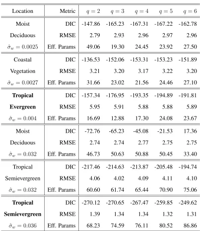
the deviance information criterion (DIC). DIC can be thought of as the Bayesian analog of Akaike information criterion (AIC), where the number of parameters in AIC is replaced by an estimate of the effective number of parameters in DIC (Spiegelhalter et al. 2002). Estimates of DIC, RMSE, and the effective number of parameters for models withq = 2, . . . ,6are presented in Table 1 for six example locations ranging in degree of inter-annual variability (characterized by the estimated posterior mode ofσw from a model withq = 3parameters).

In general, we found that the sensitivity of SV I1:T to the included harmonics in the model

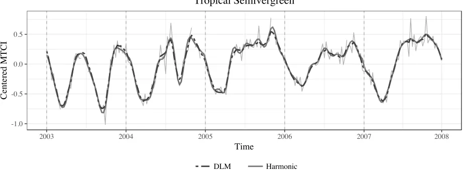
see for example the values calculated for the bottom three locations included in Table 1, and the proportion of credible intervals which did not contain 0 forq >3harmonics were generally small (< 0.2). For these locations, the DLM represents key features in the time series using fewer harmonics than a non-dynamic model and is less prone to small fluctuations that can occur as an artifact from including higher order harmonics in the model. Figure 3 illustrates this by comparing the estimated posterior medianSV I1:T from theq = 3DLM to the estimated mean from aq = 6

harmonic regression (the latter fitted separately to each year of data).

For locations which exhibit little change in seasonality across years, the DLM provided a simi-lar fit to aq-harmonic regression model and therefore, the choice of included harmonics had higher influence onSV I1:T. We found that, in general, the proportion of credible intervals not containing

zero was small for harmonics beyond the first three in theq = 6DLM for the majority of consid-ered locations of this type, with a few locations suggesting the inclusion of the4th harmonic. A similar conclusion was drawn comparing DIC across models, where for most considered locations the decrease in DIC from q = 3 to q = 4 harmonics was small (see for example the first two locations in Table 1). However, for a small number of considered locations, there was a moderate decrease in DIC fromq= 3toq= 4harmonics as exhibited in the third location included in Table 1. For these locations, we ultimately determined that it was preferable to fit a model with slightly fewer (q = 3) harmonics than a larger number, as including additional harmonic terms does not necessarily increase the flexibility of the DLM. In fact, a model with fewer harmonics will often be more flexible than a model including higher order harmonics. This is illustrated by the fact that the effective number of parameters may decrease, and/or RMSE may increase, when more parameters are added to the model. In these cases, the model with a smaller number of harmonics is more flexible since in the DLM a larger evolution variance allows the DLM to accommodate deviations away from a strictly periodic cycle. In Table 1, the decrease in effective number of parameters can be seen in the first three locations from q = 2 to q = 3, and the fourth location illustrates that RMSE can increase as harmonics are added to the model.

Figure 4 compares the posterior median ofSV I1:T (top) and estimated timings of events and

1. The estimated timings of events, in particular, were fairly robust to the choice ofq, as demon-strated by the similarity in estimates forq > 2in both locations. In summary, using the reduced Fourier-form DLM we found that we were reasonably able to capture seasonality and estimate SOS and POG over the majority of locations using the firstq = 3harmonics. While we could have considered further tuning the number of harmonics for each location, the decision to fit a model with the same number of harmonics to all locations is motivated by finding a parsimonious model that allows an automatic implementation for a large number of locations.

4.2

Convergence and Effective Size

For each natural vegetation grid cell, we estimated the reduced Fourier-form model withq = 3

harmonics, s = 46, c1 = 0.1, and c2 = 0.1, initially running two MCMC chains, in parallel,

for 10,000 iterations. Computation time for a complete analysis (from data to phenological event summaries) for one location took≈1.5 min on a 2.6 GHz Intel Core i5 processor. Convergence of MCMC algorithm was assessed (results not shown) using trace plots and ergodic means for a sample of locations, and by monitoring the Gelman-Rubin diagnostic for all locations since a visual analysis of convergence for over 1,000 locations was unrealistic.

For locations exhibiting clear variability in seasonality, the chains appeared to converge within 1,000 iterations, but in locations with little variability, the chains tended to take longer to converge due to small values causing poor mixing in the chains of σw. For these locations, an additional

10,000 iterations were sampled in each chain, to better sample the posterior. The chains were then thinned after burn-in to retain 4,000 samples for estimating the timings of SOS and POG. Inference about summaries of POG and SOS are of primary interest, so autocorrelation in posterior samples of POG and SOS calculated fromM draws ofSV I1:T was also investigated. The effective sample

sizes for POG and SOS were calculated using thecodapackage inR(Plummer et al. 2006), and found to be nearly equal toM, suggesting little to no autocorrelation in samples of POG and SOS.

4.3

Summary of Findings

months), andk = 3(suggesting that difference in MTCI value between SOS and peak growth must be at least three times more than the estimated standard deviation of the observation error). The values were chosen based on visual assessment for the purpose of illustrating the methodology, but could easily be tuned further given scientific information.

To determine the number of growing seasons per year, we computed the estimates of the prob-abilities in (3) forg = 0, . . . ,3using 4000 draws from the posterior distribution at each natural vegetation location. The number of POG’s identified in one year defines the number of growing seasons, so under our rule the probability in (3) has the specific form

ˆ

pd(g) = 1

M

M X

i=1

I(# ofP OG(i)in yeard=g) (4)

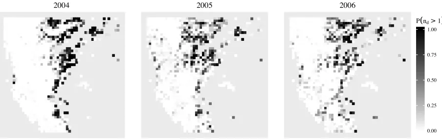
Maps of the estimated probability for each location that two or more growing seasons (pˆd(2) + ˆ

pd(3)) were identified by the algorithm for years d = 2004 - 2006 are shown in Figure 5.

Inter-estingly, the probability of identifying two or more growing seasons appeared to increase between 2004 and 2005 in the western side of the region. This change can be seen in the time series at many locations in this area, suggesting a shift occurred in the phenology between 2004 and 2005. It is unclear whether this change was due to anthropogenic activity or natural occurring events.

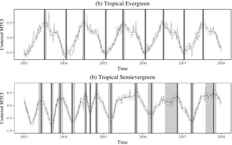
Conditional on the number of growing seasons per year, point estimates of POG and SOS were calculated as the median timing of thei= 1, . . . , M_d∗ posterior values of POG(i), SOS(i)for each year,d, and uncertainty in the estimates is expressed using 90% quantile intervals. Figure 6 presents posterior median estimates and 95% credible intervals forSV I1:T, as well as point

in 2005-2007 as the seasonal structures become plateau-like, making POG difficult to identify precisely.

Averaging across estimates obtained from implementing the methodology on each included location, first SOS in 2005 averaged 5.7 days earlier than in 2004, but in 2006 averaged 9.8 days later than in 2005. These differences are not outside the estimated uncertainty in estimates of SOS and POG, however. The majority of SOS estimates in 2004-2006 had interval widths ranging from 16 to 80 days and the majority of estimated POG had interval widths ranging from 24 to 160 days. Note that since the temporal unit of the data is an 8-day composite, the smallest possible interval width is 8 days. In general, SOS was more precisely estimated than POG. Approximately 80% of estimated SOS had a 90% interval width of 48 days or less, while only about 65% of POG estimates had intervals with widths at least that small.

5

Conclusions and Future Work

The approach presented in this paper based on a Bayesian analysis of DLMs provides a natural environment to model and extract phenological patterns from time series of satellite derived VI data, and is a flexible extension of currently applied methods. The methodology is also extendable to other types of satellite sensor data, when the objective is to characterize growth cycles or features of growth cycles. The recursive estimation procedures of Bayesian DLMs using the Kalman Filter and FFBS easily handle missing values, even when data are missing for sequential time points. This eliminates the need to preprocess and impute missing values, and incorporates time dependence to better inform the distribution of states at times when data are missing. Using MCMC simulation of the model, we developed methods to assess the number of growing seasons per year using estimated probabilities and additionally were able to provide uncertainty intervals with estimates of the timings of phenological events, which is novel in this area to our knowledge.

The model utilized in this paper can be extended to allow for more complex modeling. We have assumed a lack of systematic long term trend across years; a constant evolution of both the state and observation equations (by imposing constant V = σ_e2 and constantW = σ2_wI); and all harmonics included in the model evolve with the same variance,σ2

easily relaxed by adding a either a time-varying or constant mean/trend component to the model. Relaxing the assumption of constantV to time-varyingVt may be beneficial since time series of

MTCI data seem to exhibit higher variability, or noise, around POG, with inter-annual changes in the magnitude of this variation, particularly in locations with a marked shift in the phenology. This suggests possible dynamic evolution of the observation equation variance. Investigating more flexible specifications ofWtis also of interest.

un-certainty assessment, and the need for continued work to address the complexities of space-time non-stationarity in phenology.

6

Acknowledgements

We are grateful to the NERC Earth Observation Data Centre for providing the MTCI data. We thank the Editor, Associate Editor and Referee for valuable comments that led to substantial improvements in the paper. This work was partially supported by the National Science Foundation (DMS-1638521).

References

Agrawal, S., Joshi, P. K., Shukla, Y., and Roy, P. S. (2003), “SPOT vegetation multi temporal data for classifying vegetation in south central Asia,”Current Science, 84(11), 1440–1448.

Atkinson, P. M., Jeganathan, C., Dash, J., and Atzberger, C. (2012), “Inter-comparison of four models for smoothing satellite sensor time-series data to estimate vegetation phenology,”Remote Sensing of Environment, 123, 400–417.

Banerjee, S., Carlin, B. P., and Gelfand, A. E. (2014), Hierarchical Modeling and Analysis for Spatial Data, 2 edn, Boca Raton, FL: Chapman and Hall/CRC.

Carter, C. K., and Kohn, R. (1994), “On Gibbs Sampling for State Space Models,” Biometrika, 81(3), 541–553.

Cressie, N., and Wikle, C. (2011),Statistics for Spatio-temporal Data, Hoboken, N.J: Wiley.

Dash, J., and Curran, P. J. (2004), “MTCI: The MERIS Terrestrial Chlorophyll Index,” Interna-tional Journal of Remote Sensing, 25(23), 5403–5413.

Dash, J., and Curran, P. J. (2007), “Evaluation of the MERIS terrestrial chlorophyll index (MTCI),” Advances in Space Research, 39(1), 100–104.

Index to study spatio-temporal variation in vegetation phenology over India,”Remote Sensing of Environment, 114, 1388–1402.

De Beurs, K. M., and Henebry, G. M. (2010), “Spatio-Temporal Statistical Methods for Modelling Land Surface Phenology,” inPhenological Research: Methods for Environmental and Climate Change Analysis, eds. M. R. Keatley, and I. L. Hudson, New York: Springer, chapter 9, pp. 177– 208.

Duncan, J., Dash, J., and Atkinson, P. (2015), “The potential of satellite-observed crop phenol-ogy to enhance yield gap assessments in smallholder landscapes,” Frontiers in Environmental Science, 3(56).

Eddelbuettel, D., and Franc¸ois, R. (2011), “Rcpp: Seamless R and C++ Integration,” Journal of Statistical Software, 40(8), 1–18.

Fr¨uhwirth-Schnatter, S. (1994), “Data Augmentation and Dynamic Linear Models,” Journal of Time Series Analysis, 15(2), 183–202.

Gamerman, D. (2010), “Dynamic Spatial Models Including Spatial Time Series,” inHandbook of Spatial Statistics, Boca Raton, FL: CRC Press, pp. 437–448.

Geerken, R. A. (2009), “An algorithm to classify and monitor seasonal variations in vegetation phe-nologies and their inter-annual change,”ISPRS Journal of Photogrammetry and Remote Sensing, 64, 422–431.

Geerken, R., Zaitchik, B., and Evans, J. P. (2005), “Classifying rangeland vegetation type and coverage from NDVI time series using Fourier Filtered Cycle Similarity,”International Journal of Remote Sensing, 26(24), 5535–5554.

Gelfand, A. E., and Banerjee, S. (2017), “Bayesian Modeling and Analysis of Geostatistical Data,” Annual Review of Statistics and Its Application, 4(1), 245–266.

Hanes, J. M., Liang, L., and Morisette, J. T. (2014), “Land Surface Phenology,” in Bio-physical Applications of Satellite Remote Sensing, ed. J. M. Hanes, Springer Remote Sens-ing/Photogrammetry, : Springer Berlin Heidelberg, pp. 99–125.

Jeganathan, C., Dash, J., and Atkinson, P. M. (2010a), “Characterising the spatial pattern of phe-nology for the tropical vegetation of India using multi-temporal MERIS chlorophyll data,” Land-scape Ecology, 25, 1125–1141.

Jeganathan, C., Dash, J., and Atkinson, P. M. (2010b), “Mapping the phenology of natural vegeta-tion in India using a remote sensing-derived chlorophyll index,”International Journal of Remote Sensing, 31(22), 5777–5796.

J¨onsson, P., and Eklundh, L. (2004), “TIMESAT – a program for analyzing time-series of satellite sensor data,”Computers & Geosciences, 30, 833–845.

Kalman, R. E. (1960), “A New Approach to Linear Filtering and Prediction Problems,” Transac-tions of the ASME–Journal of Basic Engineering, 82(Series D), 35–45.

Kandasamy, S., and Fernandes, R. (2015), “An approach for evaluating the impact of gaps and mea-surement errors on satellite land surface phenology algorithms: Application to 20 year NOAA AVHRR data over Canada,”Remote Sensing of Environment, 164, 114–129.

O’Connor, B., Dwyer, E., Cawkwell, F., and Eklundh, L. (2012), “Spatio-temporal patterns in veg-etation start of season across the island of Ireland using the MERIS Global Vegveg-etation Index,” ISPRS Journal of Photogrammetry and Remote Sensing, 68, 79–94.

Petris, G., Petrone, S., and Campagnoli, P. (2009), Dynamic Linear Models with R, Use R!, : Springer New York.

Plummer, M., Best, N., Cowles, K., and Vines, K. (2006), “CODA: Convergence Diagnosis and Output Analysis for MCMC,”R News, 6(1), 7–11.

R Core Team (2015), R: A Language and Environment for Statistical Computing, R Foundation for Statistical Computing, Vienna, Austria.

Sakamoto, T., Yokozawa, M., Toritani, H., Shibayama, M., Ishitsuka, N., and Ohno, H. (2005), “A crop phenology detection method using time-series MODIS data,”Remote Sensing of Environ-ment, 96(3–4), 366–374.

Schmidt, A. M., Guttorp, P., and O’Hagan, A. (2011), “Considering covariates in the covariance structure of spatial processes,”Environmetrics, 22(4), 487–500.

Spiegelhalter, D. J., Best, N. G., Carlin, B. P., and Van Der Linde, A. (2002), “Bayesian measures of model complexity and fit,” Journal of the Royal Statistical Society: Series B (Statistical Methodology), 64(4), 583–639.

Tan, B., Morisette, J. T., Wolfe, R. E., Gao, F., Ederer, G. A., Nightingale, J., and Pedelty, J. A. (2011), “An Enhanced TIMESAT Algorithm for Estimating Vegetation Phenology Metrics From MODIS Data,” IEEE Journal of Selected Topics in Applied Earth Observations and Remote Sensing, 4(2), 361–371.

Vrieling, A., de Beurs, K. M., and Brown, M. E. (2011), “Variability of African farming systems from phenological analysis of NDVI time series,”Climatic Change, 109(3), 455–477.

Vrieling, A., De Leeuw, J., and Said, M. Y. (2013), “Length of growing period over Africa: Vari-ability and trends from 30 years of NDVI time series,”Remote Sensing, 5(2), 982–1000.

West, M., and Harrison, J. (1999),Bayesian Forecasting and Dynamic Models, Springer Series in Statistics, : Springer New York.

(a) Tropical Evergreen (b) Tropical Semievergreen

2003 2004 2005 2006 2007 2008 2003 2004 2005 2006 2007 2008 -1.0

-0.5 0.0 0.5

-0.5 0.0 0.5

Time

MTCI

Figure 1: Time series of MTCI for two sample pixels. (a) is an example of a location exhibiting little change in seasonality, while (b) shows inter-annual variability in seasonality over time.

2.0 2.4 2.8 3.2

Jan Feb Mar Apr May Jun Jul Aug Sep Oct Nov Dec Jan

Time of Year

M

TCI

Agricultural Natural Vegetation

Peak of Greenness

Peak of Greenness

Onset of 1st Crop _{Onset of 2nd Crop}

Onset of Greenness

Peak of Greenness

Location Metric q = 2 q= 3 q= 4 q = 5 q = 6

Moist Deciduous

ˆ

σw = 0.0025

DIC -147.86 -165.23 -167.31 -167.22 -162.78

RMSE 2.79 2.93 2.96 2.97 2.96

Eff. Params 49.06 19.30 24.45 23.92 27.50

Coastal Vegetation

ˆ

σw = 0.0027

DIC -136.53 -152.06 -153.31 -153.23 -151.89

RMSE 3.21 3.20 3.17 3.22 3.20

Eff. Params 31.66 23.02 21.56 24.46 27.10

Tropical

Evergreen

ˆ

σw = 0.004

DIC -157.34 -176.95 -193.35 -194.89 -191.81

RMSE 5.95 5.91 5.88 5.88 5.89

Eff. Params 16.69 12.88 17.30 24.08 23.67

Moist Deciduous

ˆ

σw = 0.032

DIC -72.76 -65.23 -45.08 -21.53 17.36

RMSE 2.74 2.74 2.77 2.75 2.75

Eff. Params 46.73 50.63 50.88 50.45 33.40

Tropical Semievergreen

ˆ

σw = 0.032

DIC -217.46 -214.63 -213.87 -205.48 -194.74

RMSE 4.06 4.02 4.09 4.11 4.10

Eff. Params 60.60 61.74 65.44 70.90 75.06

Tropical

Semievergreen

ˆ

σw = 0.036

DIC -270.12 -270.65 -267.47 -259.85 -249.62

RMSE 1.39 1.34 1.34 1.32 1.31

Eff. Params 68.23 74.59 76.11 80.52 86.86

Table 1: Deviance Information Criterion (DIC) , root mean squared error (RMSE) and effective number of parameters (Eff. Param) calculated for models withq = 2, . . . ,6included harmonics for six example locations. Three locations (top) correspond to time series where there is very little inter-annual variability, quantified by estimatedσw from the model with q = 3 parameters.

The other three locations (bottom) have relatively large estimated σw from the q = 3 model,

-1.0 -0.5 0.0 0.5

2003 2004 2005 2006 2007 2008

Time

Centered MTCI

DLM Harmonic

Tropical Semivergreen

q = 2 q = 3 q = 4 q = 5 q = 6 q = 2 q = 3 q = 4 q = 5 q = 6

−0.5 0.0 0.5

2004 2005 2006

(a) Centered MTCI −1.0 −0.5 0.0 0.5

2004 2005 2006

(b)

Centered MTCI

q = 6 q = 5 q = 4 q = 3 q = 2

q = 2 q = 3 q = 4 q = 5 q = 6

q = 6 q = 5 q = 4 q = 3 q = 2

q = 2 q = 3 q = 4 q = 5 q = 6

−2 −1 0 1 2

2004 2005 2006

(c)

Centered MTCI

q = 6 q = 5 q = 4 q = 3 q = 2

q = 2 q = 3 q = 4 q = 5 q = 6

q = 6 q = 5 q = 4 q = 3 q = 2

q = 2 q = 3 q = 4 q = 5 q = 6

q = 6 q = 5 q = 4 q = 3 q = 2

q = 2 q = 3 q = 4 q = 5 q = 6

−2 −1 0 1 2

2004 2005 2006

(d)

Centered MTCI

q = 2 q = 3 q = 4 q = 5 q = 6 q = 2 q = 3 q = 4 q = 5 q = 6

Figure 4: Plots (a)-(b) show posterior median estimates ofSV I1:T for DLMs withq = 2, . . . ,6for

2004 2005 2006

0.00 0.25 0.50 0.75 1.00 P(nd>1)

-0.5 0.0 0.5

2003 2004 2005 2006 2007 2008

Time

Centered MTCI

(b) Tropical Evergreen

-1.0 -0.5 0.0 0.5

2003 2004 2005 2006 2007 2008

Time

Centered MTCI

(b) Tropical Semievergreen

Figure 6: Example of phenological variable estimation for the two sample locations in Figure 1. Posterior median estimates of SV I1:T (dashed) with 95% credible intervals (dotted) are plotted.

(a) Evergreen (b) Semievergreen Year Estimate Interval Estimate Interval

2003 Jul 12 - 19 Jul 04 - Aug 04 Jun 10 - 17 May 17 - Jul 03 Dec 03 - 10 Nov 17 - Jan 03

2004 Jul 11 - 18 Jun 25 - Jul 26 Jul 27 - Aug 03 Jul 11 - Aug 03 Oct 31 - Nov 07 Oct 23 - Nov 23

2005 Jul 04 - 11 Jun 26 - Jul 27 Nov 01 - 08 Oct 16 - Nov 24 2006 Jul 12 - 19 Jun 04 - Jul 27 Nov 17 - 24 Jul 28 - Dec 02 2007 Jul 12 - 19 Jun 04 - Jul 27 Oct 16 - 23 Aug 05 - Nov 16