Grid Power Optimization Based on Adapting Load Forecasting and Weather Forecasting for System Which Involves Wind Power Systems

Grid Power Optimization Based on Adapting Load

Forecasting and Weather Forecasting for System Which

Involves Wind Power Systems

Fadhil T. Aula, Samuel C. Lee

School of Electrical and Computer Engineering, University of Oklahoma, Norman, USA. Email: {fadhil.aula,samlee}@ou.edu

Received December 29th_{, 2011; revised February 27}th_{, 2012; accepted March 4}th_{, 2012}

ABSTRACT

This paper describes the performance, generated power flow distribution and redistribution for each power plant on the grid based on adapting load and weather forecasting data. Both load forecasting and weather forecasting are used for collecting predicting data which are required for optimizing the performance of the grid. The stability of each power systems on the grid highly affected by load varying, and with the presence of the wind power systems on the grid, the grid will be more exposed to lowering its performance and increase the instability to other power systems on the gird. This is because of the intermittence behavior of the generated power from wind turbines as they depend on the wind speed which is varying all the time. However, with a good prediction of the wind speed, a close to the actual power of the wind can be determined. Furthermore, with knowing the load characteristics in advance, the new load curve can be determined after being subtracted from the wind power. Thus, with having the knowledge of the new load curve, and data that collected from SACADA system of the status of all power plants, the power optimization, load distribution and redistribution of the power flows between power plants can be successfully achieved. That is, the improvement of performance, more reliable, and more stable power grid.

Keywords: Wind Power Systems; Grid; Power Plants; Wind Forecasting; Load Forecasting; Power Optimization

1. Introduction

In general, a power grid involves many and different power systems that together supply power to the custom- ers. The performance and availability of the generated power are varied from system to another. Usually, a steam power system with fuel sources like nuclear or coal pro- vides the baseload which requires operating most of the time with approximately constant generating power. Fur- thermore, the steam power system needs longer time for responding to the load changes. On the other hand, natural gas power system, usually, responds faster to load changes. However, the steam turbine can be used for building large power plants which can produce more power than other power systems [1].

The economic issues and environmental impact of the conventional power systems which are using fossil fuels are not encouraging to adding more of these systems on the grid to cover the increase of the demand of the elec- trical loads. Furthermore, the global direction is to use the renewable power sources for building the power not just for covering the increasing demand of the power, but also to eliminate the usage and substitute the fossil power sys-

tems. Wind power is leading the other renewable power sources for generating electrical power and it is expected to reach or more than 20% of total global generated elec- trical power by 2030. Different modifications have been applied to wind turbines for improving their performance and increasing their efficiency. However, the intermit- tence of the generated power due to change of the wind makes the wind power system suffer from smoothly working with other power systems on the grid [2].

In this paper, a technique has been presented and im- plemented for regulating the grid, and minimizing the ef- fect of variation of the generated power of the wind power systems. The technique which is used is based on knowing in advance the load data and the generated power of the wind power systems. The data for the load is predicted based on the knowledge of the previous recorded grid load and nature of customers and the generated wind power is predicted by good knowledge of the weather forecast in the areas where wind farms are located.

generated wind power; a technique for load redistribution; and conclusion.

2. Load Predicting and Customers Usage

Accurate data for electric power load forecasting are es- sential for operating and planning of utility companies. The power industry requires forecasts for production as well as for financial perspective. It is necessary to predict hourly loads as well as daily peak loads. Accurate track- ing of the load by the system generation at all times is a basic requirement in the operation of power systems and must be accomplished for various time intervals. Since electricity cannot be stored efficiently in large quantities, the amount of the power which is generated at any given time must cover all of the demand from consumers as well as grid loss [3].

Forecasts of the load are used to decide whether extra generation must be provided by increasing the output of online generators, by committing one or more extra units, or by the interchange of power with neighboring systems. Similarly, forecasts are used to decide whether the output of an already running generation unit should be de- creased or switched off.

Load forecast can be divided into three categories: short, med, and long terms. Short term forecasting which usually starts from one hour to a week. Med term fore- casting is from a week to a year. The load forecasting more than a year counted as a long term. For short term load forecasting several factors should be considered such as time factors, weather data, and possible custom- ers’ classes. The med and long terms of the load fore- casting take into account the historical load and weather data, the number of customers in different categories, the appliances in the area and their characteristics including age, the economic and demographic data and their fore- casts, the appliance sales data, and other factors.

The time factors include the time of the year, the day of the week, and the hour of the day. There are important differences in load between weekdays and weekends. On the other hand, most electric utilities serve customers of different types such as residential, commercial, and in- dustrial [4].

In this paper, the short term load forecasting is adapted to the grid power management since the grid contains wind power systems. Usually, the perdition of the gener- ated power from the wind turbine is more accurate in short time rather than long term at least with the current weather forecasting technologies. Different techniques are available for modeling the short term load forecasting. For instance, time series have been used for a long time in load forecasting [5], the load forecasting output of artificial neural network as a model which is compen- sated by rough set theory for better accuracy [6], and the

back propagation of neural network [7-9]. In general, the artificial neural network has been proven to be reliable in prediction errors, but very large historical recorded data is required. Fuzzy logic technique, on the other hand, does not need huge historical recorded data for predicting process [10-12].

The main object of the short term load forecasting is to advise dispatcher in making a decision to:

 Supply load with stability aspect and consistence;

 Estimation full allocation;

 Determine operation constraints;

 Updating the system;

 Determine equipment limitation; and

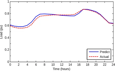
 Power management between different power systems. However, the best estimation of the short term load forecasting process is collecting historical data. These data should be classified as day of the week, as weekends usually have lower load than other weekdays, also the coordinate temperature and weather condition, the season and the day time. Taken into account that load will in- crease from year to another as number and type of cus- tomers are changing. A typical load forecasting and ac- tual load are shown in Figure 1 [13].

3. Weather Forecasting Collecting Data

Global numerical weather prediction (NWP) models, which have been in place since 1950 [14], are the core of weather forecasting as they carry out most of the data assimilation process and produce the initial and boundary conditions used by limited area models. These models are based on equations governing the motions and forces affecting motion of fluids. From the knowledge of the actual state of the atmosphere, the system of equations allows to estimate what the evolution of state variables will be at a series of grid points. These variables are tem- perature, velocity, humidity and pressure which are needed as input for estimating and predicting the wind power generating.

0 2 4 6 8 10 12 14 16 18 20 22 24 0

0.2 0.4 0.6 0.8 1

Time (hours)

Lo

ad

(

pu

)

Predict Actual

Wind forecast for wind energy applications rely most on wind speed and direction at 50 m to 100 m from ground level, at the top of the atmosphere surface layer, and only marginally on the forecast of air density. In general, the conversion of available wind power which is proportional to the cube of the wind’s speed into actual power varies nonlinearly. When wind speed is below 3 m/s the power which generated from wind will be zero and is known as cut-in speed region. The generated pow-er growth rapidly and gets its nominal rating when the wind speed is around 15 m/s where this region is known as rated-speed region which will be extended un- til cut-off speed region occurs, some new modern tur- bines are designed in no cut-off speed. The cut-off speed, usu-ally, occurs when wind speed exceeds 25 m/s [15].

There are two models for short-term wind forecast, Rapid Update Cycle (RUC) and North American Meso- scale (NAM). The RUC is designed to provide numerical giddiness for a very short term forecast to users [16]. The features of RUC are as following:

 Maximum forecast length is 12 hr (its expanded to 18 hr in 2010);

 The forecast is issued every hour starting at 00, 03, 06, 09, 12, 15, 18 and 21 UTC;

 Provide very high frequency updates of current con- ditions and short-range forecasts.

The NAM model is designed to provide short term weather forecast numerical guidance, day-ahead [17]. The general features for this model are:

 Maximum forecast length of 84 hr;

 A day-ahead forecast;

 Forecast values updated every 3 hrs.

The combination of both models is implemented in this research providing a 24 hrs a head wind speed fore- cast.

4. Behavior of Power Plants on the Grid

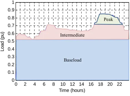
Regarding to load demand curve, power plant operation is conventionally broken down into different timescale ranging from seconds to days. Power plants which are responding within minutes load variations are partly loaded plants respond through governor action. Power plants re- sponding to this timescale are known as baseload provider. The peak and intermediate provider in the time-scale in-volves the plants that balance the load increasing and de-creasing. This portion of timescale covers several minutes to several hours according to the demand on the basis of power plants operation strategies [18]. Figure 2 shows a

typical timescale load demand curve based on Figure 1.

In general, baseload power systems involve large scale hydropower systems, coal power systems, gas power sys- tems and nuclear power systems, except for scheduled maintenances or repairs, these power plants will be in

0 2 4 6 8 10 12 14 16 18 20 22 0

0.1 0.2 0.3 0.4 0.5 0.6 0.7 0.8 0.9 1

Time (hours)

Load (

pu

)

Baseload Intermediate

Peak

Figure 2. Timescale load demands.

duties all the times. Since these power plants are slow to start up and shut down, they work more efficiently to pro- vide baseload. Furthermore, the baseload power plants are responsible for generating the most available power on the grid.

On the other hand, the peak and intermediate loads are supplied by smaller power systems like diesel, oil or nat-ural gas fired power systems. The behaviors of these small power plants meet the requirement of the peak and intermediate load which occurred in periods and varies from time to time. These power plants can be brought on line and shut down quickly.

In contrast to the other power plants, renewable power systems, such as wind power systems and solar power systems, are not considered to serve neither baseload nor peak or intimidate loads as they produce power interme- diately. However, they are effective in helping to reduce the need for fossil power systems.

5. Generated Wind Power Expectation

The expectation of the generated power from a wind tur- bine depends on the wind speed forecasting data. In gen- eral, the power in the wind turbine is proportional to:

 The cube of the wind speed, v (m/s);

 The area of wind turbine being swept by the wind, A (m2_{) ;}

 The air density, ρ (kg/m3_{) ;}  Generator efficiency, ηg;  Gear box bearing efficiency, ηb;

 The coefficient of performance of the wind machine,

Cp (Cpmax = 0.59).

Thus, the wind power can be defined as:

3 1

2 p g b

P Av C   (1)

where, P is available power, in watts, from the wind ma- chine.

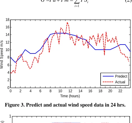
speed. Therefore, the accurate estimation of the gener- ated power depends on the accuracy of the wind speed forecasting. In this paper and for the research purpose, the wind speed forecasting data has been collected in more than weather forecast sources [19,20], and these data are compared with the actual real time data in the same time frame and the same region where wind farm is installed [21]. Figure 3 shows the forecast and actual

wind speed data, and Figure 4, depicts the corresponding

generated power from wind power system, where the wind turbine has the following parameter values, blade length (30 m), Cp (0.4), air density (1.23 kg/m3), genera-

tor efficiency (0.9), and neglecting gear box losses.

6. Redistribution Technique of the Load

The power grid requires equilibrium between demanding loads and generating power. However, the reliable power system requires having a total installed capacity to be larger than load demands. Thus, the net capacity always has safe margin for unexpected temporary load increase. The following expression shows the relation between grid and other net components;

1

n i i

G Pa Pm PS



  



0 2 4 6 8 10 12 14 16 18 20 22

0 2 4 6 8 10 12 14 16 18

Time (hours)

W

in

d

S

p

ee

d

m

/s

Predect Actual

Figure 3. Predict and actual wind speed data in 24 hrs.

0 2 4 6 8 10 12 14 16 18 20 22

0 0.2 0.4 0.6 0.8 1

Time (hours)

W

ind

P

ower

G

ene

rat

ion (

pu)

Predect Actual

Figure 4. Predict and actual wind power generation (base power is 1.667 MVA).

where, G is a grid capacity, Pa is available operation system power, Pm is a margin safe power, PSi is power

plant i, and n is number of plants on the grid.

The balance between demanding loads and grid capac- ity is;

1 1

n m

i

i j

PS L

 

 _j





and,

1 1

n m

i

i j

PS Pm L

 

  _j





where, Lj is a load at point j, and m is the total available

loads.

The vision for the future load demands and availability of the total net capacity even for a short term will be very necessary to distribute loads between different power plants. Based on the knowledge of the behavior of the each plant, economic impact, availability and readiness of the plant, programmed maintenances, and weather and seasons, the total capacity of the net can be decided. On the other hand, the reliable and efficient system per- formances of the power grid depend on the good expec- tation of the load and power system sources. Furthermore, the future power grid is in direction to include more wind power systems, thus the good prediction of the wind speed will also be another important factor for increasing the grid performance. Depending on the current weather forecasting technologies and the best load forecasting methods give the 24 hours to 48 hours ahead the most accurate collecting future data. Hence, the regulation and correction of distribution and redistribution during this period will be at minimum, and this process for another consecutive period can be done without interruptions.

During the operation, some power systems, for exam- ple steam power plant, are used to supply baseload which require minimum variation with the load. These types of power system need long time to respond to the load varia- tions, start, and shut down. However, these types usually supply large portion of the load. On the other hand, there are power systems, for example hydropower system, that suitable for fast responding to the load variation.

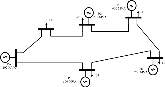
For case study, assume the following power systems are available on the grid; steam power plant (Ps), hydro- power plant (Ph), gas power plant (Pg), diesel power plant (Pd), and wind power system (Pw). The diagram of a typical grid with rated power for each plan is shown in

Figure 5. Thus, the relation can be written as;

1

n i i

G PS Ps Ph Pg Pd P







Ps 600 MVA Pg

200 MVA

Ph 200 MVA

Pd 600 MVA Pw

202 MVA

L1

L2 L3

L4 L5

Figure 5. Grid diagram.

wind power should be predicted according to the weather forecasting. The generation power of the wind power systems and the load are both varied with the time. Then, they can be subtracted from each other to form a new load curve.

Therefore, we can write the following relations;



Pa G Pw





(6)



Pm G Pw (7)

1 m

j j

Pa L Pw







The variation of the wind power generation with the wind speed leads Pa and Pm have variable values too. Equations 6 and 7, with the base of G = 1234 MVA, yield to;





Pm  p u

and,





Pa  p u

Figure 6 which is based on Figure 2 shows the actual

and predict of the load after subtracted from wind power to give the vision of the real load demand on the grid with the presence of the wind farm.

From Figure 5, the load can be equally divided be-

tween power systems as;

600 200 600 200

600 32 600 202

Ps Ph Pg

Pd Pw

 

  (9)

From Equations (2) and (5), and using the values in (9), we get;

2.05667

G Ps

g

(10) Therefore, the maximum contribution of each power

plants to the gird is; Ps = 48.6%, Ph = 16.2%, Pg = 16.2%, Pd = 2.6%, and Pw = 16.4%.

Now, Let Ps and Pg be the baseload provider. There- fore, Lmin ≥ Ps + Pg, where Lmin is a minimum load on

curve load (Figure 6). The distribution of the load will

be given by;

min if min

L Ps Pg L Ps P (11)

and,

min if min

L Ps Pg Ph Pd   L Ps Pg (12)

Since the baseload provider is 64.8% which is greater than the minimum point on load curve Lmin (Figure 6).

Thus, from Equation 11 the load distribution between Ps

and Pg is;

min 4 3 , or 0.75 min, and 0.25 min

L  Ps Ps L Pg L (13) From the load curve in Figure 6, Lmin = 0.5, therefore,

according to Equation 13; Ps = 0.375, and Pg = 0.125. These two values represent the continuous operation for both Ps and Pg at 462.75 MVA and 154.25 MVA, re- spectively. However, these values will be constant as long as the following expression is true;

 

L t   Pd Ph (14)

In case the result of Equation 14 returns false, the re- distribution process of the load will be done. Here, Equa- tion 12 can be written as;

 

L t Ps Pg Pd Ph   (15)

Using the algorithm in [22] with eliminating the solar power system in the network, and using MATLAB simu- lation the following relationships, Figure 7, show the dis-

Pa Pm

0 2 4 6 8 10 12 14 16 18 20 22 0

0.2 0.4 0.6 0.8 1

Time (hours)

Loa

d-W

ind

P

o

w

e

r (pu)

Predict Actual

Figure 6. Predict and actual load-wind power characteristic.

0 2 4 6 8 10 12 14 16 18 20 22

0 0.2 0.4 0.6 0.8 1

Time (hours)

P

ow

e

r (

pu)

Predict Actual

0 2 4 6 8 10 12 14 16 18 20 22 0

0.2 0.4 0.6 0.8 1

Time (hours)

P

o

w

e

r (pu)

Predict Actual

(a) (b)

0 2 4 6 8 10 12 14 16 18 20 22

0 0.2 0.4 0.6 0.8 1

Time (hours)

Po

w

e

r (

p

u

)

Predict Actual

0 2 4 6 8 10 12 14 16 18 20 22

0 0.02 0.04 0.06 0.08 0.1

Time (hours)

P

o

w

e

r (

pu)

Predict Actual

(c) (d)

0 2 4 6 8 10 12 14 16 18 20 22 0

0.2 0.4 0.6 0.8 1

Time (hours)

Po

w

e

r (

p

u

)

Predict Actual

0 2 4 6 8 10 12 14 16 18 20 22

0 0.2 0.4 0.6 0.8 1

Time (hours)

P

o

w

e

r (

pu)

Predict Actual 1

(e) (f)

Figure 7. Simulation results. (a) Steam power plant; (b) Gas power plant; (c) Gas power plant; (d) Diesel power plant; (e) Total generated power (not included wind power system); (f) Wind power system.

In comparison between Figures 6 and 7(e), there is a

difference between generated power and load. The gen-

sion lines losses, transformer losses, and etc. on the grid.

7. Conclusions

In this paper, the load forecasting and wind speed fore- casting are adapted in the power system which involves wind power system. The case study that implemented in the simulation consists of 15% wind power system in total of grid power. The load distribution and re-distribution between different power systems gave the optimization of the generated power. Thus, the influence from the inter- mediate behavior of the wind power systems is minimized through good estimation of the 24 hrs ahead wind and load forecasting. The simulation results show the behavior of the steam and gas turbine while they provide baseload, and other systems in intermediate and peak loads. The achievement of optimization has been successful since the grid previously prepared for distribution load, and the correction due to errors in forecasting take place without disturbance to the baseload or influence to the balance between available capacity and load demands.

This work may be extended to include other renewable power systems such as solar power system. Also, it may adapt weather forecast directly from the forecast centers.

REFERENCES

[1] S. Kaplan, “Power Plants: Characteristics and Costs,” Fed- eration and American Scientists, CRS Report or Congress, 2008.

[2] Department of Energy of USA, “20% Wind Energy by 2030,” Energy Efficiency and Renewable Energy, 2008. [3] M. Espinoza, J. Suykens, R. Belmans, and B. De Moor,

“Electric Load Forecasting Using Kernel-Based Model- ing,” IEEE Control Systems, Vol. 27, No. 5, 2007, pp. 43- 57.

[4] H. L. Willis, “Spatial Electric Load Forecasting,” Marcel Dekker, New York, 1996.

[5] G. E. P. Box and G. M. Jenkins, “Time Series Analysis: Forecasting and Control,” Prentice Hall, Saddle River, 1970.

[6] P. Qingle and Z. Min, “Very Short-Term Load Forecast- ing Based on Neural Network and Rough Set,” Interna- tional Conference on Intelligent Computation Technology and Automation, Vol. 3, Changsha, 11-12 May 2010, pp. 1132-1135.

[7] A. G. Bakirtzis, V. Petridis, S J. Kiartzis, M. C. Alexiadis, and A. H. Maissis, “A Neural Network Short-Term Load Forecasting Model for the Greek Power System,” IEEE Transactions on Power Systems, Vol. 11, No. 2, 1996, pp.

858-863. doi:10.1109/59.496166

[8] D. Papalexopoulos, S. Hao and T. M. Peng, “An Imple- mentation of a Neural Network Based Load Forecasting Model for the EMS,” IEEE Transactions on Power Sys- tems, Vol. 9, No. 4, 1994, pp. 1956-1962.

doi:10.1109/59.331456

[9] R. Afkhami-Rohani, T. L. Lu, A. Abaye, M. Davis and D. J. Maratukulam, “ANNSTLF-A Neural Network-Based Electric Load Forecasting System,” IEEE Transactions on Neural Networks, Vol. 8, No. 4, 1997, pp. 835-846. doi:10.1109/72.595881

[10] H. Chen, C. A. Canizares and A. Singh, “ANN Based Short- Term Load Forecasting in Electricity Markets,” Proceed- ings of the IEEE Power Engineering Society Transmis- sion and Distribution Conference, Vol. 2, Columbus, 28 Jaunary-1 February 2001, pp. 411-415.

[11] Z. Baharudin, M. F. Jamaluddin and N. Saad, “Fuzzy Logic Technique for Short Term Load Forecasting,” BICET, Darussalam, August 2005.

[12] Z. Baharudin, N. Saad and R. Ibrahim, “A Fuzzy Logic Technique for Short Term Load forecasting,” 2nd ICAIET, Kuala Lumpur, 3-5 August 2004, pp. 63-67.

[13] PJM Interconnection LLC. www.pjm.com/

[14] J. Charney, R. Fjortoft and J. von Neumann, “Numerical Integration of the Barotropic Vorticity Equation,” Tellus, Vol. 2, No. 4, 1950, pp. 237-254.

doi:10.1111/j.2153-3490.1950.tb00336.x

[15] C. Monteiro, et al., “Wind Power Forecasting: State-of- the-Art 2009,” Institute for Systems and Computer Engi- neering of Porto (INESC Porto) and Decision and Infor- mation Sciences Division, Argonne National Laboratory, Argonne, 2009.

[16] M. Lange and U. Focken, “Physical Approach to Short- Term Wind Power Prediction,” Springer-Verlag, Berlin, Heidelberg, 2006.

[17] A. Kusiak, H.-Y. Zheng and Z. Song, “Wind Farm Power Prediction: A Data-Mining Approach,” Wind Energy, Vol. 12, No. 3, 2009, pp. 275-293. doi:10.1002/we.295 [18] L. Freris and D. Infield, “Renewable Energy in Power

Systems,” John Wily and Sons, Hoboken, 2008. [19] Earth Networks, WeatherBug, 2011.

http://weather.weatherbug.com

[20] AccuWeather, Inc., 2011. http://www.accuweather.com/ [21] Weather Underground, 2011.

http://www.wunderground.com