Finite Difference Implicit Schemes to Coupled Two Dimension Reaction Diffusion System

(1)

http://www.scirp.org/journal/jamp ISSN Online: 2327-4379

ISSN Print: 2327-4352

DOI: 10.4236/jamp.2018.64066 Apr. 20, 2018 737 Journal of Applied Mathematics and Physics

Finite Difference Implicit Schemes to Coupled

Two-Dimension Reaction Diffusion System

Shahid Hasnain

1

, Muhammad Saqib

2

, Nawaf Al-Harbi

1

1_{Department of Mathematics, Numerical Analysis Division, King Abdulaziz University, Jeddah, KSA} 2_{Department of Mathematics, Air University, Islamabad, Pakistan}

Abstract

In this research article, two finite difference implicit numerical schemes are described to approximate the numerical solution of the two-dimension mod-ified reaction diffusion Fisher’s system which exists in coupled form. Finite difference implicit schemes show unconditionally stable and second-order accurate nature of computational algorithm also the validation and compari-son of analytical solution, are done through the examples having known ana-lytical solution. It is found that the numerical schemes are in excellent agree-ment with the analytical solution. We found, second-implicit scheme is much faster than the first with good rate of convergence also we used NVIDA de-vices to accelerate the computations and efficiency of the algorithm. Numeri-cal results show our proposed schemes with use of HPC (High performance computing) are very efficient and reliable.

Keywords

Crank Nicolson, Taylor’s Series, Richardson Extrapolation and Alternating Direction Implicit

1. Introduction

Reaction diffusion (RD) equations rise up naturally in systems consisting of many interacting factors, such as chemical reactions and are widely used to identify pattern formation phenomena in diverseness of biological and physical systems [1]. The primary ingredients of all these models are in the form of mathematical balance equation [1] which is in two dimensions

( )

2

( )

,

tu u u

∂ =

β

∇ +R (1)

where u=u x y t

(

, ,

)

is a vector of concentration variables, R(u) describes a local

How to cite this paper: Hasnain, S., Saqib, M. and Al-Harbi, N. (2018) Finite Difference Implicit Schemes to Coupled Two-Dimension Reaction Diffusion System. Journal of Applied Mathematics and Physics, 6, 737-753. https://doi.org/10.4236/jamp.2018.64066

Received: January 26, 2018 Accepted: April 17, 2018 Published: April 20, 2018

http://creativecommons.org/licenses/by/4.0/

(2)

DOI: 10.4236/jamp.2018.64066 738 Journal of Applied Mathematics and Physics

reaction kinetics and the Laplace operator _∇2_{acts on the vector}u_component

wise, also β_{denotes a diagonal diffusion coefficient matrix}_[1]_{. Noted that we}

suppose the system to be isotropic and uniform, so β_{is represented by a scalar}

matrix, independent on coordinates of the system [1]. Research in this field starts form the classical papers of [1] [2] [3], incited by population dynamics issues, where researchers made modified diffusion equation:

(

, ,

)

(

)

( )

tu x y t uxx uyy u

∂ =

β

+ +R (2)

with a nonlinear source term

( )

2

R u = −u u [2][3][4]. A typical solution of the

Equation (1), a propagating front, separating two non-equilibrium homogeneous states, one of which

(

u=1

)

is stable and another one

(

u=0

)

is unstable,

such fronts behavior is often said to be propagation into stable state and also other referred to as waves (or fronts) of transition from an unstable state [3][4] [5]. The interest in thesefronts was stimulated in the early 1980s, such as these fronts can be found in various physical, chemical as well as biological systems [5] [6].

The reaction diffusion Equation (2) represents a model equation for the evolution of a neutron population in a nuclear reactor and also arises in chemical engineering applications, such equation allows for the effects of linear diffusion by means of uxx+uyy and nonlinear local multiplication or reaction through R

( )

u [7][8].

Researchers have studied these model problems such as the stability of symmetric traveling waves in the Cauchy problem for a more general case than Equation (2); also some researchers explained perturbation method and found an approximate solution by expanding the solution in terms of a power series and in terms of some small parameters [8].

In this paper, we suggest a reaction diffusion system, which agree to several physical phenomena, the most common is the change in space and time of the concentration of one or more chemical substances. Local chemical reactions in which the metamorphosed into each other, and diffusion which causes the substances to spread out over a surface in space. Reaction diffusion systems are naturally applied in chemistry. However, the system can also describe dynamical processes of non-chemical nature. Mathematically, reaction diffusion systems take the form of semilinear parabolic partial differential equations. The general form of our proposed reaction diffusion system in two dimension, is

(

)

2

( ) (

)

, , , , 0

t xx yy

u =

β

u +u +u v−

α

u x y ∈ −∞ ∞ t≥ (3)

(

)

2

( ) (

)

, , , , 0

t xx yy

v =

β

v +v −v u x y ∈ −∞ ∞ t≥ (4)

where β is diffusion coefficient and α is a reactive factor, and u x t

( )

, is

concentration and v x t

( )

, is the velocity of the chemical reaction. The aim of this

(3)

efficiency in time. Comparison of two finite difference (FD) schemes is also mentioned with CPU efficiency.

The outlook of the paper is in Section 2 analytical solution, Section 3 smoothness and uniqueness, Section 4 numerical methods, Section 5 numerical results and Section 6 discussion.

2. Analytical Solution

To derive the analytical solution of the given system in (3), (4), we assume the solution of the two dimension coupled reaction diffusion system, in the following form

(

_{, ,}

)

_e 2 t

x y

u x y t = α − − (5)

(

_{, ,}

)

_e 2

t x y

v x y t = −α + + (6)

3. Smoothness and Uniqueness of the Reaction Diffusion

System

In order to guarantee the smoothness and uniqueness of a positive solution and to obtain upper and lower bounds of the solution, it is necessary to impose some general assumptions on the various physical parameters and the reaction function [9][10]. Throughout this paper, we always assume that the diffusion coefficientβ_{is positive in domain}Ω_{also at}t=0 the initial values u v₀, ₀ are

non-negative, where the smoothness hypothesis is used only for the existence problem of the corresponding linear system, and the non-negative hypothesis on the data is to obtain non-negative solutions [9][10]. Let us consider the system,

(

)

( )

(

)

( )

[ ]

( )

[ ]

( )

(

)

( )

(

)

( )

2 1 1 2 2 0 0 , ,

where 1, , and ,

, ,

Boundary Conditions, 0, ,

0, , ,

Initial Conditions, ,

m t

u u u f u v v v u g u v

m f u v uv g u v v B u h x y

B v h x y

t x y u x y u x y

v x y v x y x y α   − ∇ ⋅ ∇ = − _   − ∇ ⋅ ∇ = _   ≥ = − =    = _ _   = _  

> ∈Ω _

 = _ _  _ = _ _  ∈Ω _ β β (7)

motivated by the nonlinear reaction functions given by Equation (7), we make the following basic assumption on functions f and g[9][10].

3.1. Assumption or Hypothesis (H)

f v

∂ ∂ _{exists and is bounded subsets of domain}Ω_{and there exists a function with}

( )

, 0

o

c x y ≥ , such that 0≤ f u v

(

, ₁

)

≤ f u v

(

, ₂

)

≤c_o

( )

x y, for 0≤ ≤v₁ v₂≤ ∞ [9]

[10]. This definition implies that the function f is monotone non-decreasing in v

(4)

both functions f and g, thus this property leads to

(

)

( )

(

)

( )

1 2 , , , , , , , , , m m

F x y u v u f u v F x y u v u g u v



= − _



= + _ (8)

where above Equation (8) represents F F1, 2 are quasi monotone non-increasing

and quasi monotone non-decreasing functions in Ω respectively [9] [10]. According to classification of the reaction functions, F F1, 2 are typed III functions [9][10], which leads to the following definition of the solutions.

3.2. Definition

A smooth pair of two vector functions

( )

u v , ,

(

u v,

)

defined in

R

+

× Ω

are called upper and lower solutions respectively, if they satisfy the following inequalities

(

)

( )

(

)

(

)

(

)

( )

(

)

(

)

(

)

(

)

[ ]

( )

(

)

( )

2

1 1 1

2 2 2

0

, 0 , ,

where 1, , , and , ,

( , ) ( , )

Boundary Conditions, 0, ,

0, , , 0,

m m

t t

m m

t t

u u u f x v u u u f x y v v v u g x v v v u g x y v

m f x y v uv g x y v v B u h x y B u

B v h x y B u

t x y u x y u x y u x

α  − ∇ ⋅ ∇ + ≥ ≥ − ∇ ⋅ ∇ + _  − ∇ ⋅ ∇ − ≥ ≥ − ∇ ⋅ ∇ − _ ≥ = − =  ≥ ≥ _  ≥ ≥ _ > ∈Ω ≥ ≥              β β β β

(

)

(

)

( )

(

)

( )

0 ,

0, , , 0, ,

Initial Conditions, ,

y v x y v x y v x y

x y                _ ≥ ≥ _ _  ∈Ω _  (9)

In the above definitions the smoothness of

( )

u v , ,

(

u v,

)

is in the sense that

these functions are continuously differentiable to the order appeared in Equations (7) and (8) respectively [9] [10]. Hypothesis and above definition leads to the following theorem.

3.3. Theorem

Let f and g satisfy above hypothesis (H). If there exist upper and lower solutions

( )

u v , ,

(

u v,

)

of system 7, such that u≤u and v≤v in

R

+

× Ω

, then the sequence

{

u v k, k

}

,

{

u vk, k

}

converges monotonically from above and below, respectively, to a unique solution (u, v) of system (7) [9][10]. Moreover

(

) (

)

(

)

(

) (

)

(

)

( )

, , , , , ,

0, ,

, , , , , ,

u t x y u t x y u t x y

t x y v t x y v t x y v t x y

≤ ≤ _

> ∈Ω



≤ ≤ _



 (10)

(5)

qua-DOI: 10.4236/jamp.2018.64066 741 Journal of Applied Mathematics and Physics

si-monotone increasing function, the upper and lower solutions for the present system are interconnected andto be determined simultaneously from relations in Equation (9). This makes the determination of these functions more delicate, especially in relation to the stability property of non-homogeneous systems [9] [10]. Nevertheless, for the global existence problem or the stability problem with homogeneous boundary conditions the construction of those functions is not very difficult [10].

4. Numerical Methods

We consider the numerical solution of the nonlinear system in (5), (6) and (7) in a finite domain Ω =

{

( )

x y, |a< <x b c, < <y d

}

, where the first step is to

choose integers n and m to define step sizes h= −

(

b a n

)

and k=

(

d−c m

)

[11] [12]. Partition the interval [a, b] into n equal parts of width h and the interval [c, d] into m equal parts of width k and place a grid on the rectangle R

by drawing vertical and horizontal lines through the points with coordinates

(

x y_i, _j

)

, where x_i= +a ih for each i=0,1, 2,,n and yj = +c jk for each

0,1, 2,

,

j

=



m

also the lines x=x_i and y=yj are grid lines, and their intersections are the mesh points of the grid [12][13] [14][15] [16]. For each mesh point in the interior of the grid,

(

x y_i, _j

)

, for i=1, 2,,n−1 and

1, 2,

,

1 j

=



m

−

, also we assume tn=nt n, =0,1, where t is the time grid step

size [16]. We denote the analytical and numerical solutions at the grid point

(

x t_m, _n

)

by u_mn and U_mn respectively.

4.1. Second Order Implicit Scheme

The Crank Nicolson scheme for the system in (3) and (4) can be displayed as follows:

(

)

( )

1 , , 1 , ,

1, , 1,

2

, 1 , , 1

2

1, , 1,

2

, 1 , , 1

2

1 2 2 2

, , 1

, ˆ

2

ˆ 2

ˆ 2ˆ ˆ

ˆ

ˆ 2ˆ ˆ

ˆ

ˆ 2ˆ ˆ

ˆ

ˆ 2ˆ ˆ

ˆ

ˆ ˆ ˆ 0.5 ˆ 0 8

n n l m l m

l m l m l m x

l m l m l m y

l m l m l m x

l m l m l m y

n n

l m l m x y

l m

u u u

v v v

u u u u

h u u u u

h v v v v

h

k

u u u vu k u

v δ δ δ δ δ δ + + + − + − + − + − + + = + = − + = − + = − + = − + =

− −R + − + =

(

)

( )

1 2 2 2

, 1 ˆ ˆ ˆ 0,

8

n n

l m x y

k v δ δ v v u

+                      

− −R + + = _

(11)

where 1 2

k h

β

=

(6)

scheme with block linear penta diagonal structure [17] [18]. The Newton's iterative method is used to solve this linear system, such scheme is of second order accuracy in both directions, space and time respectively [17] [18]. The scheme is unconditionally stable using the von Neumann stability analysis [18].

4.2. Computationally Efficient Implicit Scheme

In search of a time efficient alternate, we analyzed the naive version of the Crank Nicolson scheme for the two dimensional equation, and find out that that scheme is not time efficient such that to get time efficiency, the common name of Alternating Direction Implicit (ADI) method can be used [19] [20]. In ADI scheme, the two steps are as follows:

(

)

2 2

, , ,

, , , ,

2 1 2

, , ,

2 2

, , ,

2 1 2

, ˆ 1 1 2 2 ˆ ˆ 1 1 2 2 ˆ 1 1 2 2 1 1 2 2 n n

x l m y l m l m

n n n n

l m l m l m l m n

y l m x l m l m

n n

x l m y l m l m

n

y l m x

r r

u u tf

f u u v

r r

u u tf

r r

v v tg

r r v δ δ α δ δ δ δ δ δ + +   ₋  _{= +}  _{+ ∆}           ₌ ₋   ₋  _{= +}  _{+ ∆} _     _       ₋  _{= +}  _{+ ∆}          ₋  _{= +}        

(

)

, , , , , , ˆ ˆ

n n n n

l m l m l m l m l m l m

g u v v v tg         _  _  _{= −} _    + ∆  _   (12)

The trick used in constructing of ADI scheme, is to split time step into two sweeps and apply two different stencils in each half time step, therefore to increment time by one time step in grid point , we first compute both of these stencils, such that the resulting linear system is block tridiagonal [20][21][22]. The scheme in Equation (12) is a nonlinear implicit scheme of second order accuracy in space and time. According to Von Neumann stability analysis, such scheme is also unconditionally stable [22][23][24][25].

4.3. Algorithm

The nonlinear system of Equation (12), can be written in the form:

( )

0,

R W = (13)

where

(

1, , ,2 3 , 2

)

t n

R= r r r  r , W =

(

u₁n+1,v₁n+1,u₂n+1,v₂n+1,,u_mn+1,v_mn+1

)

and

1, , ,2 3 , 2n

r r r  r are the nonlinear equations obtained from the system in

Equation (12). The system of Equations in (12) is solved by Newton's iterative method using the following steps:

1) Specify ( )0

W as an initial approximation.

2) For

k

=

0,1, 2,



until convergence achieve.

− Solve the linear system

( )

( )k ( )k

( )

( )k

A W ∆W = −R W

− _Specify ( )k1 ( )k ( )k

W + =W + ∆W ,

where

( )

( )k

A W is

(

m m×

)

Jacobian matrix, which is computed analytically

and ( )k

W

∆ _{is the correction vector}_[26] _[27]_{. In the iteration method solution}

(7)

stopped when

( )

( )k

R W Tol

∞≤ with Tol is a very small prescribed value. The

linear system obtained from Newton's iterative method, is solved by Gauss elimination method with partial pivoting also convergence done with iterations along less CPU time [28][29][30].

4.4. Norms

The accuracy and consistency of the schemes is measured in terms of error norms specially L2 and L∞ which are defined as:

(

)

( )

(

)

ecact Approximation ecact Approximation

1 ₁

ecact Approximation ecact Approximation

2 ₂

1

2

max

log Error Error Rate

log 2

m

j j

i m _j m

j j

j

h h

L u u u u

h h ∞ _∞ _{≤ ≤} = =   = − = −    = − = − _    = _ 

∑

(14)

Two more interesting error are listed below,

(

)

2 ecact Approximation

, ,

relative _exact2

, 2 ecact Approximation , , 2 Error

RMS , where Total terms

i j i j i j

i j j

i j i j i j u u u u u M M  − _  =      −  = = _ 

∑∑

∑

∑∑

(15)

5. Numerical Results

Numerical computations have been performed using the uniform grid, for the test problem, the approximated and analytical solutions such as u x y t

(

, ,

)

and

(

, ,

)

U x y t have been given in Table 1, Table 2 at different grids with some

fixed parameters such as

α

=1, β =1 4 and k=0.0001 and t=1 using

(8)

[image:8.595.207.538.103.197.2]

Table 1. Error comparison by crank nicolson scheme at different grid sizes, at t = 1 and time step = k = 0.0001.

Grid Size Errorrelative RMS L2 L∞

11 × 11 0.0089 0.0152 0.1671 0.0285

21 × 21 0.0091 0.0312 0.1869 0.0463

31 × 31 0.0091 0.0403 0.2139 0.0512

41 × 41 0.0095 0.0679 0.3913 0.0710

[image:8.595.207.538.240.334.2]

51 × 51 0.0099 0.0931 0.5524 0.0989

Table 2. Rate of convergence comparison by crank nicolson scheme at different grid sizes at t = 1 and time step = k = 0.0001.

Grid Size RateL2 RateL∞ L2 L∞

11 × 11 2.9385 2.0235 0.1671 0.0285

21 × 21 2.2367 1.9896 0.1869 0.0463

31 × 31 1.8976 1.4781 0.2139 0.0512

41 × 41 1.2145 1.2797 0.3913 0.0710

[image:8.595.207.540.373.466.2]

51 × 51 1.1135 1.0923 0.5524 0.0989

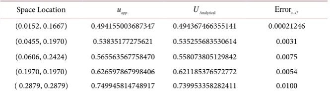
Table 3. Solution by ADI scheme at different locations at t = 1, time step = k = 0.0001 and grid size = 25 × 25.

Space Location uapp. UAnalytical Erroru U−

(0.0152, 0.1667) 0.494155003687347 0.494367466355141 0.00021246

(0.0455, 0.1970) 0.53835177275621 0.535255683530614 0.0031

(0.0606, 0.2424) 0.565563567758470 0.558073805129842 0.0075

(0.1970, 0.1970) 0.626597867998406 0.621185376572772 0.0054

[image:8.595.207.538.508.603.2]

( 0.2879, 0.2879) 0.749945814748917 0.739953358282411 0.0100

Table 4. Error comparison by ADI scheme at different grid sizes, at t = 1 and time step =

k = 0.0001.

Grid Size Errorrelative RMS L2 L∞

11 × 11 0.0741 0.0173 0.1899 0.0713

21 × 21 0.0341 0.0283 0.5934 0.0428

31 × 31 0.0123 0.0362 1.1231 0.0232

41 × 41 0.0099 0.0428 1.7538 0.0155

51 × 51 0.0090 0.0485 2.4713 0.0136

Table 5. Error comparison by ADI scheme at different time with time steps = k = 0.0001.

t = time Errorrelative RMS L2 L∞

0.01 0.00013 0.0102 1.04713 0.00198

0.05 0.00089 0.0209 1.09513 0.00589

0.1 0.0011 0.0319 1.12686 0.00989

0.5 0.0039 0.0400 1.8535 0.0109

(9)

[image:9.595.205.539.90.169.2]

Table 6. Error comparison by ADI scheme at different time steps.

k = time steps Errorrelative RMS L2 L∞

0.01 0.0484 0.2942 2.3542 0.1236

0.001 0.0483 0.2936 2.3393 0.1240

0.0001 0.0461 0.2935 2.3380 0.1241

0.00001 0.0423 0.2935 2.3378 0.1241

Table 7. Rate of Convergence Comparison by ADI scheme at different grid sizes.

Grid Size RateL2 RateL∞ L2 L∞

11 × 11 2.8009 2.8201 0.1899 0.0113

21 × 21 2.8458 2.8733 0.5934 0.0128

31 × 31 2.8619 2.8934 1.1231 0.0132

[image:9.595.207.539.199.278.2]

51 × 51 2.8458 2.8733 2.4713 0.0136

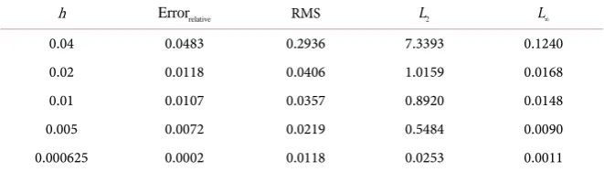
Table 8. Error Comparison by ADI scheme at different space step sizes.

h Errorrelative RMS L2 L∞

0.04 0.0483 0.2936 7.3393 0.1240

0.02 0.0118 0.0406 1.0159 0.0168

0.01 0.0107 0.0357 0.8920 0.0148

0.005 0.0072 0.0219 0.5484 0.0090

0.000625 0.0002 0.0118 0.0253 0.0011

Table 9. Interesting feathers of ADI scheme at different grid sizes.

Grid Size Self Time Total Time CTC. Function Convergence Rate

11 × 11 0.312 s 0.743 s 12,642 2.8201

31 × 31 1.094 s 2.291 s 38,322 2.8934

51 × 51 1.968 s 4.030 s 65,602 2.8733

Table 10. Interesting feathers of ADI scheme at different grid sizes.

Grid Spacing Self Time Total Time CTC. Function Convergence Rate

h 12.757 s 18.458 s 293,250 2.8201

h/2 3.18925 s 4.6145 s 73,356 2.8934

6. Discussion

[image:9.595.207.538.309.403.2]

(10)

[image:10.595.208.533.77.276.2]

Figure 1. Shows results using Crank Nicolson scheme with t = 0.1 and Grid = 25 × 25.

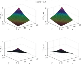
Figure 2. Shows results using Crank Nicolson scheme t = 0.3 and Grid = 53 × 53.

computational time and increase memory capacity [34][35][36]. Solving such a linear system is not practical due to extremely high time complexity of solving a linear system by the means of Gaussian Elimination method or residual technique

[image:10.595.212.532.326.583.2]

(11)

[image:11.595.212.530.76.280.2]

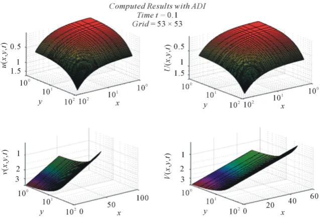
Figure 3. Shows results using ADI scheme with t = 0.1 and Grid = 53 × 53.

Figure 4. Shows results using ADI scheme with t=0.1 and Grid =53 53× with log

scaling in xy plane of u x y

( )

, and only y log scaling in v x y

( )

, .

is that the implicit solver only requires a tridiagonal matrix algorithm to be solved, so that the difference between the true Crank Nicolson solution and ADI approximated solution has an order of accuracy of

( )

2

O k and hence can be

[image:11.595.210.529.319.536.2]

(12)

[image:12.595.209.526.76.274.2]

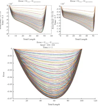
Figure 5. Shows results using CN scheme at t=0.5 and Grid=101 101× with log

scaling in xy plane for u x y

( )

, and v x y

( )

, by Crank Nicolson.

[image:12.595.213.535.331.680.2]

(13)

[image:13.595.211.539.66.465.2]

Figure 7. Shows simulations with capacity of the system along CPU usage and performance. Also processor calls and threads, by Crank Nicolson. Specification of the system is mentioned in computer applications header.

performance of the CPU for two different schemes. The derivation of our ADI scheme for a nonlinear PDE system relies on a few key observations. Most im-portantly, using the solution at time levels previous to n1

t=t + , the algorithm

converts the nonlinear spatial operator into an implicit but linear operator with variable coefficients. The resulting approximately-factored equation is solved in sweeps along each of the Cartesian directions, including, as is common in ADI approaches, an intermediate n1 2

t + step, so that all of the proposed algorithms

are embodied in the two steps formula that every iteration updated the block tri-diagonal linear algebraic system [32]-[39].

Computer Applications

(14)

[image:14.595.89.517.71.421.2]

Figure 8. Shows simulations with ADI. CPU usage increase from 9% to 13% with efficiency.

[image:14.595.80.516.451.706.2]

(15)

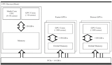
High performance computing system, by halting the traditional development to increase the clock rate, number of cores that are being increased in the system, however, many cores architecture based different powerful devices such GPU (Graphics Processing Unit) and GPGPU (General Purpose Graphics Processing Unit) by NIVIDA, MIC (Many Integrated Core) by Intel and FPGA (Field programmable Gate Array) have been introduced recently that outperform the conventional CPU processing by thousand folds [29] [38] [39]. In order to utilize these powerful devices, new software stacks, algorithms and frameworks have been introduced, ehereas the modern computing system provides massive parallelism through inter node and intra node computation where inter node processing is performed by MPI (Message Passing Interface), most popular programming model and intra node by OpenMP directive programing model

[29][38][39].

Keeping in view, the advantages of this emerging technology, we have intro-duced Crank Nicolson and ADI schemes with the help of this application by us-ing FUJITSU Primergy RX 350 S7 HPC computer havus-ing Intel Xeon E5-2667 processor of 2.80 GHz processing power which contained 16 physical cores and 32 logical cores, main memory size of 32 GB and HDD 4 TB inside it [29][38] [39], see from Figures 7-9. Moreover, we used 2 Tesla k-80 accelerated NVIDA devices that are capable to deliver not only graphical processing purpose but also for general purpose processing [29] [38][39]. However, our application struc-ture is designed for MATLAB based on hybrid of tri-hierarchy level tightly coupled programming model containing CUDA (Compute Uniform Device Architecture) for accelerated computation [29][38][39].

Acknowledgements

The authors are gratefully acknowledged Dr. Muhammad Faheem Afzaal, Department of Chemical Engineering, Imperial College London, UK and Muhammad Usman Ashraf, Department of Computer Science, King Abdulaziz University, Saudi Arabia.

Conflict of Interest

The authors do not have any conflict of interest in this research paper.

References

[1] Fisher, R.A. (1937) The Wave of Advance of Advantageous Genes. Annals of

Eu-genics, 7, 355-369. https://doi.org/10.1111/j.1469-1809.1937.tb02153.x

[2] Canosa, J.C. (1973) On a Nonlinear Diffusion Equation Describing Population Growth. IBM Journal of Research Development, 17, 307-313.

https://doi.org/10.1147/rd.174.0307

[3] Arnold, A.R., Showalter, K.S. and Tyson, J.J. (1987) Propagation of Chemical Reac-tions in Space. Journal of Chemical Education, 64, 740-743.

https://doi.org/10.1021/ed064p740

(16)

Uni-DOI: 10.4236/jamp.2018.64066 752 Journal of Applied Mathematics and Physics

versity Press, Cambridge, UK.

[5] Gazdag, G.J. and Canosa, J.C. (1974) Numerical Solutions of Fisher’s Equation.

Journal of Applied Probability, 11, 445-457. https://doi.org/10.2307/3212689

[6] Abdullaev, U.G. (1994) Stability of Symmetric Traveling Waves in the Cauchy Problem for the KPP Equation. Journal of Differential Equations, 30, 377-386. [7] Logan, D.J. (1994) An Introduction to Nonlinear Partial Differential Equations.

Wiley, New York.

[8] Evans, D.J. and Sahimi, M.S. (1989) The Alternating Group Explicit (AGE) Iterative Method to Solve Parabolic and Hyperbolic Partial Differential Equations. Annals of Numerical Fluid Mechanics and Heat Transfer, 2, 283-389.

[9] Segel, L.A. (1984) Chapter 8: Modelling Dynamic Phenomena in Molecular and Cellular Biology. Cambridge University Press, Cambridge.

[10] Pao, C.V. (1981) Asymptotic Stability of Reaction-Diffusion Systems in Chemical Reactor and Combustion Theory. Journal of Mathematical Analysis and Applica-tions, 82, 503-526. https://doi.org/10.1016/0022-247X(81)90213-4

[11] Schiesser, W.E. and Griffiths, G.W. (2009) A Compendium of Partial Differential Equation Models. Cambridge University Press, Cambridge.

https://doi.org/10.1017/CBO9780511576270

[12] Argyris, J.A., Haase, M.H. and Heinrich, J.C. (1991) Finite Approximation to

Two-Dimensional Sine Gordon Equations. Computer Methods in Applied

Me-chanics and Engineering, 86, 1-26. https://doi.org/10.1016/0045-7825(91)90136-T

[13] Aronson, D.G. and Weinberger, H.F. (1978) Multidimensional Non-Linear

Diffu-sion Arising in Population Genetics. Advance in Mathematics, 30, 33-76.

https://doi.org/10.1016/0001-8708(78)90130-5

[14] Hilborn, R.H. (1975) The Effect of Spatial Heterogeneity on the Persistence of Pre-dator-Prey Interactions. Theoretical Population Biology, 8, 346-355.

https://doi.org/10.1016/0040-5809(75)90051-9

[15] Hans, L.P. (1999) Computational Partial Differential Equations. Springer Verlag, Berlin.

[16] Hayhoe, M.N. (1978) Numerical Study of Quasi-Analytic and Finite Difference So-lutions of the Soil-Water Transfer Function. Soil Science,125, 68-79.

[17] Linker, P.L. (1990) Numerical Methods for Solving the Reactive Diffusion Equation in Complex Geometries. Technische Universität Darmstadt, Darmstadt, Hessen. [18] Tang, T.S. and Weber, R.O. (1991) Numerical Study of Fisher’s Equations by a

Pe-trov-Galerkin Finite Element Method. The ANZIAM Journal, 33, 27-38.

https://doi.org/10.1017/S0334270000008602

[19] Khaled, K.A. (2001) Numerical Study of Fisher’s Diffusion-Reaction Equation by the Sinc Collocation Method. Journal of Computational and Applied Mathematics, 137, 245-255. https://doi.org/10.1016/S0377-0427(01)00356-9

[20] Ames, W.F. (1965) Nonlinear Partial Differential Equations in Engineering. Aca-demic Press, New York.

[21] Ames, W.F. (1969) Numerical Methods for Partial Differential Equations. Barnes and Noble, Inc., New York.

[22] Noye, J.N. (1989) Finite Difference Methods for Partial Differential Equations.

North-Holland Publishing Comp. Conference in Queen’s College, University of Melbourne, Australia, 23-87.

(17)

Wavelet Galerkin Method. International Journal of Computer Mathematics, 83, 287-298.

[24] Dhawam, S.D., Kapoor, S.K. and Kumar, S.K. (2012) Numerical Method for Advec-tion Diffusion EquaAdvec-tion Using FEM and B-Splines. Journal of Computer Science, 3, 429-437. https://doi.org/10.1016/j.jocs.2012.06.006

[25] Tamseer, M.T., Srivastava, V.K. and Mishra, P.D. (2016) Numerical Simulation of Three Dimensional Advection-Diffusion Equations by Using Modified Cubic B-Spline Differential Quadrature Method. Asia Pacific Journal of Engineering Science and Technology, 2, 1-13.

[26] Fletcher, C.A. (2016) Generating Exact Solutions of the Two-Dimensional Burgers Equations. International Journal for Numerical Methods in Fluids, 3, 213-216.

https://doi.org/10.1002/fld.1650030302

[27] Hill, M.D. and Michael, R.M. (2008) Amdahl’s Law in the Multicore Era. Computer, 41, 33-38. https://doi.org/10.1109/MC.2008.209

[28] Heath, M.T. (1997) Scientific Computing, an Introductory Survey. University of Il-linois at Urbana-Champaign, Urbana and Champaign, IL.

[29] Ashraf, M.U., Fouz, F.F. and Fathy, A.E. (2016) Empirical Analysis of HPC Using

Different Programming Models. International Journal of Modern Education and

Computer Science, 6, 27-34.

[30] Busenberg, S.N. and Travis, C.C. (1983) Epidemic Models with Spatial Spread Due to Population Migration. Journal of Mathematical Biology, 16, 181-198.

https://doi.org/10.1007/BF00276056

[31] Crank, J.C. and Nicolson, P.N. (1947) A Practical Method for the Numerical Evalu-ation of Solutions of Partial Differential EquEvalu-ations of the Heat-Conduction Type.

Mathematical Proceedings of the Cambridge Philosophical Society, 43, 50-67.

https://doi.org/10.1017/S0305004100023197

[32] Lakoba, T.L. (2015) The Heat Equation in 2 and 3 Spatial Dimensions. In: MATH

337, University of Vermont.

[33] Srivastava, V.K. and Tamsir, M.T. (2012) Crank-Nicolson Semi-Implicit Approach for Numerical Solutions of Two-Dimensional Coupled Nonlinear Burgers’ Equa-tions. International Journal of Applied Mechanics and Engineering, 17, 571-581. [34] Smith, G.D. (1986) Numerical Solution of Partial Differential Equations: Finite

Dif-ference Methods. 3rd Edition, Oxford University Press, Oxford.

[35] Saber, E.N. (1999) An Introduction to Differential Equations. 2nd Edition, Springer Verlag, New York.

[36] Shalf, J.S., Sundip, D.S. and John, M.J. (2010) Exascale Computing Technology Challenges.In: Palma, J.M.L.M., Daydé, M., Marques, O. and Lopes, J.C., Eds., High Performance Computing for Computational Science—VECPAR 2010, Lecture Notes in Computer Science, Vol. 6449, Springer, Berlin, Heidelberg, 1-25.

[37] Shekhar, B.S. (2007) Thousand Core Chips: A Technology Perspective. Proceedings of the 44th annual Design Automation Conference, San Diego, CA, 4-8 June 2007, 746-749.

[38] Bajellan, A.A.A.F. (2015) Computation of the Convection-Diffusion Equation by the Fourth-Order Compact Finite Difference Method. İzmir Institute of Technolo-gy, January 2015.