Abstract—Based on a critical analysis of data analytics and its foundations, we propose a functional approach to estimate data ensemble properties, which is based entirely on the empirical observations of discrete data samples and the relative proximity of these points in the data space and hence named empirical data analysis (EDA). The ensemble functions include the non-parametric square centrality (a measure of closeness used in graph theory) and typicality (an empirically derived quantity which resembles probability). A distinctive feature of the proposed new functional approach to data analysis is that it does not assume randomness or determinism of the empirically observed data, nor independence. The typicality is derived from the discrete data directly in contrast to the traditional approach where a continuous probability density function (pdf) is assumed a priori. The typicality is expressed in a closed analytical form that can be calculated recursively and, thus, is computationally very efficient. The proposed non-parametric estimators of the ensemble properties of the data can also be interpreted as a discrete form of the information potential (known from the information theoretic learning theory as well as the Parzen windows). Therefore, EDA is very suitable for the current move to a data-rich environment where the understanding of the underlying phenomena behind the available vast amounts of data is often not clear. We also present an extension of EDA for inference. The areas of applications of the new methodology of the EDA are wide because it concerns the very foundation of data analysis. Preliminary tests show its good performance in comparison to traditional techniques.
Index Terms—data mining and analysis, machine learning, pattern recognition, probability, statistics.
I. INTRODUCTION
URRENTLY, there is a growing demand in Machine Learning, Pattern Recognition, Statistics, Data Mining and a number of related disciplines broadly called Data Science, for new concepts and methods that are centered on the actual data, the evidence collected from the real world rather than at theoretical prior assumptions which need to be further confirmed with the experimental data (e.g the Gaussian assumption). The core of the statistical approach is the
Manuscript received July 2016. This work was partially supported by The Royal Society grant IE141329/2014 “Novel Machine Learning Paradigms to address Big Data Streams”.
Plamen P. Angelov and Xiaowei Guare with School of Computing and Communications, Lancaster University Lancaster, LA1 4WA. (e-mail: {p.angelov, x.gu3}@lancaster.ac.uk)
José C. Príncipe is with Computational NeuroEngineering Laboratory, Department of Electrical and Computer Engineering, University of Florida, USA. (e-mail: [email protected])
definition of a random variable, i.e. a functional measure from the space of events to the real line, which defines the probability law [1]–[4]. The probability density function (pdf)
is, by definition, the derivative of the cumulative distribution function (cdf). It is well known that differentiation can create numerical problems in both practical and in theoretical aspects and is a challenge for functions which are not analytically defined or are complex. In reality, we usually do not have independent and identically distributed (iid) events, but we do have correlated, interdependent (albeit in a complex and often unknown manner) data from different experiments which complicates the procedure.
The appeal of the traditional statistical approach is its solid mathematical foundation and the ability to provide guarantees of performance, when data is plenty (N), and created from the same distribution that was hypothesized in the probability law. The actual data is usually discrete (or discretized), which in traditional probability theory and statistics are modeled as a realization of the random variable, but one does not know a priori their distribution. If the prior data generation hypothesis is verified, good results can be expected; otherwise this opens the door for many failures.
Even in the case that the hypothesized measure meets the realizations, one has to address the difference of working with realizations and random variables, which brings the issue of choosing estimators of the statistical quantities necessary for data analysis. This is not a trivial problem, and is seldom discussed in data analysis. The simple determination of the probability law (the measure of the random variable) that explains the collected data is a hard problem as studied in density estimation [1]–[3]. Moreover, if we are interested in statistical inference, for instance, similarity between two random variables using mutual information, the problem gets even harder because different estimators may provide different results [5]. The reason is that very likely the functional properties of the chosen estimator do not preserve all the properties embodied in the statistical quantity. Therefore, they behave differently in the finite (and even in the infinite) sample case. An alternative approach is to proceed from the realizations to the random variables, which is the reverse direction of the statistical approach. The literature has several excellent examples of this approach, in the area of measures of association. For instance, Pearson’s correlation coefficient is perfectly well defined in realizations, as well as in random variables. Likewise, Spearman’s [6], Kendal’s [7], are other examples of measures of association well defined in both the realization and the random variables. However, the problem with this approach is that the statistical properties of the
A Generalized Methodology for Data Analysis
Plamen Angelov,
Fellow, IEEE
, Xiaowei Gu, and Jose Principe,
Fellow, IEEE
measures in the random variables are not directly known, and may not be easily obtained. A good example of the latter is the generalized measure of association, which is well defined in the realizations, but not all of the properties are known in the random variables [8]. Therefore, there are advantages and disadvantages in each approach, but from a practical point of view, the non-parametric approach is very appealing because we can go beyond the framework of statistical reasoning to define new operators and still cross-validate the solutions with the available data using non-parametric hypothesis tests. A good example is least squares versus regression. One can always apply least squares to any data type, deterministic or stochastic. If the data is stochastic the solution is called regression, but the result will be the same, because the autocorrelation function is a property of the data, independent of its type. The difference shows up only in the interpretation of the solution; most importantly, the statistical significance of the result can only be assessed using regression.
A more recent alternative is to approximate the distributions using non-parametric, data-centered functions, such as particle filters [9], entropy-based information-theoretic learning [5], etc. On the other hand, partially trying to address the same problems, in 1965 L. Zadeh introduced fuzzy sets theory [10], which completely departed from objective observations and moved (similarly to the belief-based theory [8] introduced a bit later) to the subjectivist definition of uncertainty. A later strand of fuzzy set theory (data driven approach developed mainly in 1990s) attempted to define the membership functions based on experimental data. It stands in between probabilistic and fuzzy representations [11], however, this approach requires an assumption on the type of membership function. An important challenge is the posterior distribution approximation. Approximate inference can be done employing maximum a posteriori criteria which requires complex optimization schemes involving, for example, the expectation maximization algorithm [1]–[3].
In this paper, we present a systematic methodology of non-parametric estimators recently introduced in [12]–[15] for discrete sets using ensemble statistical properties of the data derived entirely from the experimental discrete observations and extend them to continuous spaces. These include the
cumulative proximity (q), centrality (C), square centrality (q-1),
standardized eccentricity ( ), density ( ) as well as typicality, () which can be extended to continuous spaces, resembling the information potential obtained from Parzen windows [1]–[4] in Information Theoretic Learning (ITL) [5]. Its discrete version sums up to 1 while its continuous version integrates to 1 and is always positive; however, its values are always less than 1 unlike the pdf values that can be greater than 1. Additionally, the typicality is only defined for feasible values of the independent variable while the pdf can extend to infeasible values, e.g. negative height, distance, weight, absolute temperature, etc. unless specifically constraint [12]– [15]. We further consider discrete local () and global (D)
versions. Then, we introduce an automatic procedure for identifying the local modes/maxima of D as well as a procedure
for reducing the amount of the local maxima/modes and extend the non-parametric estimators to the continuous domain by introducing the continuous global density, and typicality,
G, which further involves integral for normalization.
Furthermore, we demonstrate that the continuous global typicality does integrate to 1 exactly as the traditional pdf
(while being free form the restrictions the latter has). This is a new and significant result which makes continuous global typicality an alternative to the pdf. This strengthens the ability of the empirical data analysis (EDA) framework for objectively investigating the unknown data pattern behind the data and opens up the framework for inference. The methodology is exemplified with a Naïve EDA classifier based on G.
II. THEORETICAL BASIS - DISCRETE SETS
In this section, we start by presenting EDA foundations in discrete sets [12]-[15] for completeness and further clarity. Firstly, let us consider a real metric space RK and assume a particular data set or stream
1, 2,...,
KN
N R
x x x x ; with
T ,1
,
,2,...,
,i
x
ix
ix
i K
x
; i1, 2, , N , where subscriptsdenote data samples (for a set) or the time instances when they arrive (for a stream). Within the data set/stream, some data samples may repeat more than once, namely, xi xj,i j . The set of sorted unique data samples, denoted by
u
LN
u u
1,
2,...,
u
LN
(where
N
L N
u x , 1LN N ) and the number of occurrence, denoted by
f
LN
f f
1,
2,...,
f
LN
can be determined automatically based on the data. With
N
L
u and
N
L
f , the primary data set/stream
N
x can be reconstructed. In the remainder of this paper, all the derivations are conducted in the nth time instance
except when specifically declared otherwise. The most obvious choice of RK , is the Euclidian space with the Euclidean distance, but we can also extend EDA definitions to Hilbert spaces, and Reproducing Kernel Hilbert spaces. We can, moreover, consider different types of distances within these spaces motivated by the purposes of the analysis that exploit information available from the source that generated the samples or definitions that are appropriate for data analysis. Within EDA, we introduce:
a)cumulative proximity, q [12]–[15]; b)square centrality, ;
c)eccentricity, ξ [12]–[15];
d)standardized eccentricity, ε [12]–[15]; e)discrete local density, D [12]–[15]; f)discrete local typicality, [14], [15]; g)discrete global typicality, D [14], [15];
h)continuous local density, DL;
i) continuous global density, DG, and
j) continuous globaltypicality, G.
DG
D
1
The discrete global typicality, D addresses the global
properties of the data and will be introduced in the next section. For inference, the continuous local (DL), global density(DG)
and the continuous global typicality, (G) will be described in
detail in section IV.
A. Cumulative Proximity and Square Centrality
For every point xi
x N; i1, 2,...,N one may want toquantify how close or similar this point is to all other data points from
N
x . In graph theory, centrality is used to indicate the most important vertices within a graph. A measure of centrality [16], [17] is defined as a sum of distances from a point xi to all other points:
1
1
; ; 1 ; 1
,
N i N i N N
i j j
c i N L
d
x x x
x x
(1)
where d x x
i, j
is the distance/similarity between xi andj
x , which can be, but not limited to Euclidean, Mahalanobis, cosine, etc.
Its importance comes from the fact that it provides centrality information about each data sample in a scalar or vector form. We previously defined [12]–[15] the cumulative proximity
N i
q x as,
2
1
, ; ; 1
N
N i i j i N N
j
q d L
x x x x x (2)
which can be seen as inverse centrality with a square distance
Cumulative proximity [12]–[15] is a very important association measure derived empirically from the observed data without making any prior assumptions about their generation model and plays a fundamental role in deriving other EDA quantities. The complexity for computing the cumulative proximities ofall samples in
N
x is
2O N . As a result, the computational complexity of other EDA quantities for
N
x , which can be derived directly from cumulative proximity is
O N . For many types of distance/similarity, i.e. Euclidean distance, Mahalanobis distance, cosine similarity, etc., with which the cumulative proximity can be calculated recursively [14], the complexity for calculating the cumulative proximities
of all the samples in
N
x is reduced to O N
as well. In a very similar manner, we can consider square centralityas the inverse of the cumulative proximity, defined as follows:
1
2
1
1
; 1
,
N i N N
i j j
q L
d
x
x x
(3)
B. Eccentricity
The eccentricity, N, defined as a normalized cumulative proximity, is another very important association measure derived empirically from the observed data without making any
prior assumptions about their generation model [12]–[15]. It
quantifies data samples away from the mode, useful to represent distribution tails and anomalies/outliers. It is derived by normalizing qN and taking into account all possible data samples. It plays an important role in anomaly detection [14], [15] as well as for the estimation of the typicality as it will be detailed below. The eccentricity (N ) of a particular data sample xi in the set
N
x (LN 1) is calculated as follows [12]–[15]:
2
1
2
1 1 1
2 ,
2
; 1
,
N
i j j
N i
N i N N N N
N j j h
j h j
d q
L
q d
x x x
x
x x x
(4)
where the coefficient 2 is included to normalize eccentricity
between 0 and 1, i.e.:
0N xi 1 (5) Here, we also introduce standardized eccentricity, ε, which does not decrease as fast as eccentricity with the increase of the amount of data, N and is calculated as follows:
1
2
; 1
1
N i
N i N i N N
N j j
q
N L
q N
x
x x
x
(6)
Based on the expression of the standard eccentricity
(namely, equation (6)) one can see that the data samples which are far away from the majority tend to have higher standard eccentricity values compared with others. Thus, the standard eccentricity can serve asan effective measure of the tail of data distribution without the need of clustering the data in advance. Combining the standard eccentricity with the well-known
Chebyshev inequality [18], which discribes the probability that certain data sample x is more than n ( denotes the standard deviation) distance away from the mean, we get the EDA version of the Chebyshev inequality as follows [12], [14]:
2
2
1
1 1
N
P n
n
x (7)The Chebyshev inequality expressed by the standard eccentricity provides a more elegant form for anomaly detection. For example, if N
x 10, x has exceeded the3 limitation, and can be categorized as an anomaly.
C. Discrete Local Density
Discrete local density is defined as the inverse of
standardized eccentricity and plays an important role in data analysis using EDA (i1, 2,...,N L; N 1):
2
1 1 1
1
2
1
,
2
2 ,
N N N
N j j l
j j l
N i N i N
N i
i l l
q d
D
Nq
N d
x x x
x x
x
x x
(8)
For example, if the Euclidean distance is used, the density
2T
1
1
N i
i N N N N
D
X
x
x
(9)
where N is the mean of
N
x ; XN is the mean of
TN
x x
;N
and XN can be updated recursively using [19]:
1 1 1
T T
1 1 1 1
1 1
; ;
1, 2,...,
1 1
; ;
k k k
k k k k
k
k k
k N
k
X X X
k k
x x
x x x x
As we can see from equation (9), the discrete local density
itself can be viewed as a univariate Cauchy function while there is no assumption or any pre-defined parameter involved in the derivation besides the definition of the distance function (Euclidean distance used here).
D. Discrete Local Typicality
Discrete local typicality was firstly introduced in [13], and called unimodal typicality. In this paper, it is redefined as the normalized local density (i1, 2,...,N L; N 1):
1
1
1 1
N i N i
N i N N
N j N j
j j
D q
D q
x x
x
x x
(10)
The discrete local typicality resembles the traditional unimodal probability mass function (pmf), but it is automatically defined in the data support unlike the pmf which may have non-zero values for infeasible values of the random variable unless specifically constraint.
The discretelocal density resembles membership functions of a fuzzy set having value of 1 for
x =
while the discrete local typicality resembles pmf with the sum of NNvalues being equal to 1 and values for both D and being from the interval [0,1].As an example, the square centrality, standardized eccentricity, discretelocal density and typicality of real climate dataset (wind chill and wind gust) measured in Manchester, UK for the period 2010-2015 [20] are presented in Supplementary Fig. 1. In these examples, Euclidean distance is used.
III. THEORETICAL BASIS: DISCRETE GLOBAL
TYPICALITY In this section, we will consider the more realistic case when data distributions
are multimodal.
Traditionally, this requires identifying local peaks/modes by clustering, expectation maximization, optimization, etc. [1]–[3], [21]–[23]. Within EDA, the discrete global
typicality (τD) is derived automatically from the data with no
user input and can quantify multimodality. It is based on the
local cumulative proximity, square centrality, eccentricity and
standardized eccentricity. The only requirements to define the
discrete global typicality are the raw data and the type of distance metric (which can be any).
A. Discrete Global Typicality
Expressions (9)-(10) provide definitions of local operators that are very appropriate to quantify the peak point (x) of unimodal discrete functions. Moreover, if the peak coincides with the global mean N (xN), then the value of the
local density is equal to 1: DN
N 1. A similar property having a maximum, though its value is1, is also valid for the traditional probability by definition and according to the central limit theorem [1]–[3]. In reality, data distributions are usually multimodal [21]–[24], therefore the local description should be improved. In order to address this issue, the traditional probability theory often involves mixture of unimodal distributions, which requires estimation of number of modes and it is not easy [24]. Within the EDA framework, we provide the discrete global typicality, τD, directly from the dataset,which provides multimodal distributions automatically without the need of user decisions and only requires a threshold for robustness against outliers.
The discrete global typicality of a unique data sample is expressed as a combination of the normalized discrete local density weighted by the corresponding frequency of occurrence of this unique data sample (i1, 2,...,LN;LN 1) :
1
1
1 1
N N
j N i i N i
D
N i L L
j N j j N j
j j
f q f D
f D f q
u u
u
u u
(11)
where 1
N i
q u and DN
ui are the square centrality and thediscrete local density of a particular data sample, ui calculated from
N
L
u only .
This expression is very fundamental, because, in fact, it combines information about repeated data values and the scattering across the data space, and resembles the well-known membership functions of fuzzy sets. We further explain this link in a publication that is currently under review [25].
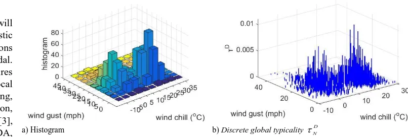
[image:4.612.146.549.586.722.2]a) Histogram b) Discreteglobal typicalityND
One can easily appreciate from Fig. 1, the differences between the D
N
and histogram with a quantization step equal to 5 for both dimensions. Note that, the histogram requires the selection of one parameter (the quantization step) per dimension, while none is needed for the discrete global typicality. For large dimensions (D), this can be a big problem. The size of the grid/axis is a user-specified parameter. The histogram takes only values from a finite set 0;1 ; 2; ;1
N N
, while D N
can take any real value.
The discrete global typicality has the following properties:
i) sums up to 1;
ii) the value is within
0,1 ;iii) provides a closed analytic form, equation (11);
vi) there is no requirement for prior assumptions as well as any user- or problem-specific threshold and parameters;
v) is free from some peculiarities of traditional probability theory (its value never gets 1 and non-zero positive for infeasible values [14], [15]) ;
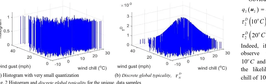
vi) can be recursively calculated for various types of metrics. When all the data samples in the dataset have different values ( fi 1; i), and the histogram quantization step parameter is not properly set, the histogram is unable to show any useful information, while the discrete global typicality can still show the mutual distribution information of the dataset, see Fig. 2 (a) and (b). This is a major advantage of discrete globaltypicality
because it is parameter free. Here the figures are based on the unique data samples of the same climate dataset. As we can see, the data samples which are closer to the mean of the dataset will have higher value of global typicality and vice versa.
It is also interesting to notice that for equally distant data, the
discrete global typicality, D N
is exactly the same as the frequentistic form of probability. Then equation (11) reduces to
1
N
L D
N i i j j
f f
u . Supplementary Fig. 2 shows a simple example of the discrete global typicality D
N
and pmf of an artificial climate dataset
50
x with only data of wind chill, which have 2 unique data samples,
50 10; 20
u (oC ),
while
50f
20; 30
.Obviously, q2
u1
2 2
q u d2
u u1, 2
, and
2
10
D o
C
0.4 ;
2
20
D o
C
0.6 .Indeed, if 20 times we observe wind chill is
10o
C and 30times 20o C
the likelihood for wind chill of 10oCwill be
40%
and for wind chill of 20oC
will be
60%
, respectively.The discrete global typicality 100D of the outcome of
throwing dices for 100 times is presented in Supplementary Fig. 3 as an additional illustrative example. In this experiment, for 1, we can use
1; 0; 0; 0; 0; 0;
T, for 2, we can use
T0; 1; 0; 0; 0; 0; , etc. Let the outcome of throwing dices 100 times be
6
17 14 15 15 21 18
; ; ; ; ;
100 100 100 100 100 100
f
, the values
of the discrete global typicality D N
of the six outcomes are equal to their corresponding frequencies, see the Supplementary Fig. 3.
B. Identifying Local Modes of Discrete Global Typicality
In this sub-section, an automatic procedure for identifying all local maxima of the discrete global typicality, defined in the previous sub-section will be described. It results in the formation of data clouds (samples associated with the local maxima) [19], [26]. Data clouds are free shape while clusters, are usually hyper-spherical, hyper-ellipsoidal. This data partitioning resembles Voronoi tessellation [27]. They are also used in the AnYa type neuro-fuzzy predictive [19], [26], classifiers and controllers.
The illustrative figures in this section are based on the same climate dataset [20] that was used earlier in Fig. 1, which has two features/attributes: wind chill (oC) and wind gust (mph). In all cases, the Euclidean distance is used, though, the principle is valid for any metric.
The proposed algorithm can be summarized as follows: Step 1: Identifying the global maximum of the discrete global typicality D
N
For every unique data sample of the dataset
N
x , its
discrete global typicality D
N i u (i1, 2,...,LN ) can be calculated using equation (11).
The data sample with the highest D N
is selected as the reference data sample in the ranked collection
*N
L
u :
*(1)
1,2,..., arg max
N
D N i j L
u u (12)
D N
[image:5.612.56.500.58.199.2]
(a) Histogram with very small quantization (b) Discrete global typicality, NDwhere *(1)
u is the data sample with the highest value of discrete global typicality (in fact, the global maximum), and we set
*m *(1)
u u . In case when there are more than one maxima, we can start with any one of them.
Step 2: Ranking the discrete global typicality D N
Then, we find the unique data sample that is nearest tou*m denoted by u*(2) and put it into
*N
L
u , meanwhile, remove it from
N
L
u . u*(2) is set to be the global maximum
*m *(2)
u u .
The ranking operation continues by finding the next data sample, which is closest to u*m , putting it into
*N
L
u , removing it from
N
L
u and setting it as the new global maximum.
By applying the ranking operation until
N
L
u becomes empty, we can finally get the ranked unique data samples, denoted as
* *( )| 1, 2,...,
N
i
N
L i L
u u and their
corresponding ranked discrete global typicality collection:
*
*(1),
D D
N N
N
u
u D
*(2) ,..., D
*(LN)
N N
u
u .Step 3: Identifying all local maxima
The ranked discrete global typicality is filtered using equation (13) to detect all local maxima of D
N
:
* 1 * * * 1
*
j j j j
D D D D
N N N N
j D
N
IF AND
THEN is a local maxma of
u u u u
u
(13) We denote the set of the local maxima (can be used as a basis for forming data clouds and, further, AnYa type fuzzy rule-based models [19], [26]) of D
N
as the set
**N
P
u
**( )
|
1, 2,...,
j
N
j
P
u
; PN is the number of the identified local maxima and PN LN.The ranked discreteglobal typicality is depicted in Fig. 3(a), the corresponding local maxima are depicted in Fig. 3(b).
Step 4: Forming data clouds Each local maxima, ** i
u , is then set as a prototype of a data cloud. All other data points are assigned to the nearest prototype (local maximum) forming data clouds using equation (14).
**( )
1,2,...,arg min ,
N
j j P
winning label d
x u (14)
Data clouds can be used to form AnYa models [19], [26]. After all the data samples within
N
x are assigned to the data clouds, the center (mean) j
N
, the standard deviation j N
and support j
N
S ( j1, 2,...,PN) per cloud can be calculated. Step 5: Selecting the main local maxima of the discrete global typicality, D
N
We then calculate D
N
at the data cloud centers, denoted by
N using equation (11) with the corrpesonding supports as their frequencies. Then, we use the following operation to take out the less prominent local maxima.For each center i N
, we check the condition (i j, 1, 2,...,
N
P ; i j):
2
i j i D i D j
N N N N N N N
i N R
IF AND
THEN
(15)
This condition means that if there is another center with higher D
N
located within the 2 i N
area of i N
, this new more prominent center replaces the existing one. This condition guarantees that the influence areas of neighboring data clouds
will not overlap significantly (it is well known that according to the Chebyshev inequality for arbitrary distribution the majority of the data samples (>75%) lie within 2 distance from the mean [1]–[3]).
By finding out all the centers satisfying the above condition and assigning them to
R
, we get the filtered data cloud
centers denoted by
*
*
* * *
| 1, 2,..., ;
N
j
N N N N
P j P P P
by excluding
R
from
N
P
(
* *
N N R P
P
and
*
*N R
P
), where *N
P is the number of remaining centers.
After that, we set
*** *
N N
P P
u
,*
N N
P P and repeat Steps 4-5 until the data cloud
centers do not change any more.
Finally, we can get the composed result, re-named as
o , and use the
o as the prototypes to(a) Ranked discreteglobal typicalityND (b) Local maxima/peaks/modes of
D N
build data clouds using equation (14).
The final data cloud centers for each selection round is presented in the Supplementary Video, which can also be downloadable from:
https://www.dropbox.com/s/kkq8xztya3u3kh1/Supplementary _Video.pptx?dl=0.
The final result is presented in Fig. 4. Compared with Fig. 3(b), in the final round, there are only two main modes left broadly corresponding to the two main seasons in Northern England and all the details are filtered out.
Even if f1 1, i , the discreteglobal typicality can still be extracted successfully from the data samples, despite the fact that the result may not be exactly the same because of the changing data structure, see Supplementary Fig. 4, which uses the same real climate dataset in Fig. 4.
The summary of automatic mode identification algorithm is as follows.
Automatic mode identification algorithm:
i. Calculate D
N i u , i1, 2,...,LN using equation (11);
ii. Find the unique data sample u*(1) with global maximum of
D N
using equation (12);
iii. Send u*(1) into
*N
L
u and
ND
u
*(1) into
*
N
D N
L
u
and delete u*(1) from
*N
L
u ;
iv. u*mu*(1);
v. While
N
L
u
* Find the unique data sample(s) which is/are nearest to
*m
u ;
* Send the data sample(s) and the corresponding D
N i u
into
*N
L
u and
*
N
D N
L
u
;* Delete data sample(s) from
N
L
u ; * Set the latest element in
*N
L
u as u*m;
vi. End While vii. Filter
*N
P
u and
*
N
D N
P
u
using equation (13) andobtain
**N
P
u as centers of data clouds;
viii. While
**N
P
u are not fixed * Use
**N
P
u and form the data clouds from
N
x
using equation (14);
* Obtain the new centers
N
P
standard deviations
N
P
and supports
N
P
S of the data clouds;
* Calculate
ND
Nj , j2,...,PN using equation (11); * Find
R
satisfying equation (15); * Exclude
R
from
N
P
and obtain
* *N
P
;*
**
* *N N
P P
u
;* *
N N
P P ;
ix. End While
x.
**N
o
P
u
;ix. Build the data clouds with
o using equation (14);C. Properties of EDA Operators
Having introduced the basic EDA operators, we will now outline their properties.
✓They are entirely based on the empirically observed experimental data and their mutual distribution in the data space;
✓They do not require any user- or problem-specific thresholds and parameters to be pre-specified;
✓They do not require any model of data generation (random or deterministic), only the type of distance metric used (however, it can be any);
✓The individual data samples (observations) do not need to be independent or identically distributed (iid); on the contrary, their mutual dependence is taken into account directly through the mutual distance between the data samples;
✓The method does not require infinite number of observations and can work with just a few exemplars; Within EDA, we still can consider cross validation and non-parametric statistical tests based on the realizations of experimentally observed data similarly to the significance tests utilized on the random variable assumed in the traditional probability theory and statistics. As a conclusion, EDA can be seen as an advanced data analysis framework which can work efficiently with any feasible data and any type of distance or similarity metric.
IV. THEORETICAL BASIS - CONTINUOUS DENSITY AND TYPICALITY
Up to this point, all EDA definitions are useful to describe data sets or data streams made up of a discrete number of observations. However, they cannot be used for inference because they are only defined on points where samples occur (discrete spaces). In this section, we define the continuous local and global density and global typicality which can be Fig.4. Final filtering result (The black ‘*’ denotes the centers of the data
used for inference on the continuous domain of the variable x. At this stage, we depart from the entirely data based and assumptions-free approach we used so far, however, this is done after we identified the local modes, formed data clouds
around these focal points and obtained the support of these data clouds. Therefore, the extension to the continuous domain is inherently local (per data cloud). We assume that the local mode considered as the mean and the support considered as frequency plus the deviation of the empirical data do provide the triplet of parameters (μ, X, Ni). We do recognize that these
triplets are conditional on the specific Nidata samples observed
and associated with the particular data cloud, but this will be updated when new data is available. Now, having this triplet of parameters we, firstly, define the continuouslocal density, L
D
as:
1
; 1
2
N N j j
N i N
N i
q
D L
Nq
x x
x (15) Like equation (9), for the case of Euclidean distance, the
continuous local density, DL is simplified to a continuous Cauchy type function over any feasible value of the variable x with the parameters μ and X extracted from N available data samples as described earlier:
, 2
, 2
, 1
; 1, 2,..., ; 1
1
L
N i N N
N i N i
D i C L
x
x
(16)
where
2 2
, , ,
N i
X
N i N i
; N i, and XN i, are the mean and the average value of scalar products of the data samples within the ith data cloud;N
C is the number of data clouds; the subscript N means the local densities are derived from N
observed data samples. It is obvious that with more data samples observed, the parameters will change and have to be updated regularly. Note that equation (16) is defined based on Euclidean distance. The
expression of continuous local density DL varies from the type of distance used. Nonetheless, in general, the continuous local density of the data can be expressed in the same form as the discrete local density but in the continuous space.
The continuous local density DL is defined on
the continuous space for each local maximum per data cloud.
Furthermore, we introduce the continuous global density DG
as a weighted sum of the local density of each data cloud with weights being the support (number of data samples) of the respective data cloud. Finally, we introduce the continuous global typicality
G based on DG. The continuous global densityand typicality play a similar role to the mixture of pdfs.However, the questions “how many distributions in the mixture”, “which are their parameters” and “what type of distributions” see Fig. 5 are all answered from the data directly, free from any user or problem-specific pre-defined parameters,
prior assumptions, knowledge or pre-processing techniques like the cases of clustering, EM, etc.
A. Continuous Global Density
Continuous global density is a mixture that arises simply from the metric of the space used to measure sample distance and the density of samples that exist in the space. However, it works for all types of distance/similarity metric. As we can see from equation (16) the local density is Cauchy type when the Euclidean distance is employed therefore, the simplest of the procedures is to define the continuous global density as a mixture of Cauchy distributions. The continuous global density
enables inference of new samples anywhere in the space. For any and any type of distance used, we define
continuous global density in a general form very much like the mixture distributions, as a weighted combination of continuous local densities:
1 , ,
; 1N
C L N i N i
G i
N N
S D
D L
N
x
x (17) where L,
N i
D x is the local density of in the ithdata cloud;
N
C is the number of data clouds at the Nth time instance;
,
N i
S
is the support (number of members) of the ithdata cloud based
on the available experimental/actual data. For normalization, we impose the condition ,
1
N
C N i i
S N
. The continuous global density DG is defined non-parametrically from each of the modes of the data (DL) and near the peaks; it is a very goodapproximation of DL, but it will deviate progressively from it in
trough regions. As an example, the global density for the same climate dataset used before [20] is presented in Fig. 6(a).
x
x Fig.5. The process of extracting distribution from data in EDA
(a) Continuousglobal density (b) Continuous global typicality
Compared with the
discrete local density
introduced in section II which is discrete and unimodal by definition,
G
D is more effective to detect the natural multimodal data structure such as abnormal data samples because only the data samples that are close to the larger data clouds, which can be viewed as the
main modes of the data patterns, can have higher values of
continuous global density. This feature is clearly depicted by the value of DG of those data samples located in the space between the two main modes in the figures below, while for the
local density, see Supplementary Fig. 1(c), it is exactly the opposite case.
B. Continuous Global Typicality
Having introduced the continuous global density, we can also define the continuous global typicality,
G as well. It is also defined as a normalized form of the density (similarly to the weighted typicality,
D, equation (11)) but with the use of integral instead of the sum. As stated in section II, the weighted typicality,
D is discrete and sums to 1. The global typicality is expressed as follows:
, , 1 , , 1 N N C LG N i N i
N
G i
N C
G L
N N i N i
i
S D D
D d S D d
x x xx x x x
(18)
It is important to notice that equation (18) is general and valid for any type of distance/similarity metric. For a general multivariate case, it is important to normalize the mixture of
continuouslocal densities L,
N iD x to make
G integrate to 1. By finding out the integral of the continuous global densitywithin the metric space and dividing
G by its integral, one can always guarantee unit integral, regardless the type of distance/similarity metric used.As we said before, we consider the well-known expression of the multivariate Cauchy distribution [21]–[23] to transform the
,
L N i
D x without loss of generality.
T
21 1 2 2 1 2 1 K d K K f xx x
(19)
where x
x x1, 2,...,xK
T; is the well-known mathematicalconstant and
is the gamma function; E
x ; is scalar parameter. This guarantees that:
2 1
1, 2,..., 1 2,... 1
K
K K
x x x
f x x x d x dx dx
(20)Based on (17)-(19), we introduce the normalized continuous local density as follows:
21, 1 ,
2 , 1
2 K
L L
N i K N i
K N i K D D
x x (21)
Here
N i, XN i,
N iT, N i, for the Euclidean distance. We can, finally, get the expression of the continuous global typicality, in terms of the normalized continuous global density as:
12 , , , 1 , 1 1 , 2 , , 1 1 2 N N N C K L L C
N i N i
N i
G i
N C K N i K
i
L N i
N i N i i
K
S D D
S N
S D d
x x x x x (22) For the Euclidean distance, equation (22) becomes
, 1 1 1 2 2 2 , , 2 , 1 2 1 N C N i GN K K
i N i K N i N i K S N
x x (23)The continuousglobal typicality of the real climate dataset with Euclidean distance is presented in Fig.6(b)
The comparisons between the continuous global typicality
(the modes are extracted by the approach introduced in section III), discrete global typicality, histogram and traditional pdf are presented in 2D form for visual clarity in Fig. 7 using the same the real climate dataset [20].
As shown in Fig. 7, compared with the traditional pdf using a Gaussian model,the global typicality derived directly from the dataset without any prior assumption about the number of local modes or type of distribution represents very well the two modes in the data pattern and gives results very close to what a histogram would give and significnatly better to what a single unimodal distribution would provide.
In summary, the proposed continuous global typicality has the following properties, many of which it shares with the
discreteglobal typicality introduced in section III:
G
(a) wind chill (oC) (b) wind gust (mph)
i)integrates to 1;
ii) provides a closed analytic form;
iii) no requirement for prior assumptions as well as any user or problem-specific threshold and parameters; these are derived from the data entirely;
vi) can be recursively calculated for various types of metrics. V. APPLICATIONS
A. Examples
In this subsection, we will give several examples of the
continuous global typicality, G of different datasets extracted
by the proposed automatic mode identification algorithm. The
continuous global typicality of the Seeds dataset [28] and Combined Cycle Power Plant dataset [29] and Wine Quality dataset [30] with Euclidean distance is presented in Fig. 8. As the dimensionality of the original datasets is > 2, for a better visualization, we use the principal component analysis (PCA) method [31] to reduce the dimensionality and use the first 2 principal components in the figures as the x-axis and y-axis. Supplementary Fig. 5 (a) and (b) present the G derived from
the first 1/3 and the first 2/3 the Wine Quality dataset. Supplementary Fig. 5 (c) depicts the G derived by scrambling
the order of the data samples. The continuous global typicality
G
of 2 dimensional benchmark datasets A1, S1 and S2 [32] are also presented in Supplementary Fig. 6.
If we want more details from the continuous global typicality, we can also stop the automatic mode identification algorithm described in section III early, i.e. before the final iteration, and build the continuous global typicality based on more detailed data partitioning results. The Supplementary Video referred in section III.B also depicts evolution of the
global continuous typicality based on the results of different iteration times of the proposed mode identification algorithm.
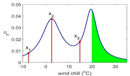
B. Inference Primer
Assuming, there are 3 arbitrary non-integer values of wind chill data x
7.5; 2.5;14.7
(oC), which does not exist in thedataset, we can quickly obtain the corresponding continuous global typicality using equation (18),
G
x
0.0080, 0.0375, 0.0180
and the inferences made are presented in Fig. 9. Here we only consider the two main modes.That means that wind chill of -7.5oC is less likely while the
wind chill of 2.5oC is more likely.
In addition, if we want to know the continuous global typicality of all the values larger than , we can integrate as follows:
T 1 G
N d
x t
x t x x (24) For example, when Euclidean distance is used, and here we only consider one-dimensional data for simpler derivation, equation (24) can be re-written as:
1 , ,
T 1
N
C L N i N i i
x t
S D x
x t dx
N
, ,
1 ,
1 1
arctan
2 1
N
C
N i N i
i N i
t S
N
(25) Let us continue the example in Fig. 9. If we want to know the
global continuous typicality of all the data samples above 20
oC, which is the green area of this figure, we can calculate the
value using equation (25) to yield T
x20
0.2447. That means that the likelihood, a value to be equal to or greater than 20 oC is 24.47%. One can see that the continuous globaltypicality can serve as a form of probability.
C. Naïve EDA Classifier
In this sub-section, we borrow the concept of naïve Bayes classifiers [1]–[3] and propose a new version of naïve EDA classifier. In contrast with the original naïve EDA classifier proposed in [15], which relies for inference on the discrete global typicality and linear interpolation and/or extrapolation, the naïve EDA classifier in this paper uses the continuous global typicality instead, which is based on the local modes of the discrete global typicality identified by an automatic procedure as described in section III.B. This procedure is more effective in reflecting the ensemble features of the distribution of the data samples of different classes in the data space.
As the proposed approach accommodates various type of distance/similarity metrics, one can use the current knowledge in the area to choose the desired distance measure for a reasonable approximation that simplifies the processing. Moreover, one can change to other distance measures easily