Dynamic Spectrum Sharing Optimization and
Post-optimization Analysis with Multiple
Operators in Cellular Networks
Md Asaduzzaman, Raouf Abozariba
*and Mohammad N. Patwary
{
md.asaduzzaman
}
,
{
r.abozariba
}
,
{
m.n.patwary
}
@staffs.ac.uk
School of Creative Arts and Engineering
Staffordshire University, Stoke-on-Trent, Staffordshire ST4 2DE, United Kingdom
Abstract
Dynamic spectrum sharing aims to provide secondary access to under-utilised spectrum in cellular
networks. The main aim of the paper is twofold. Firstly, secondary operator aims to borrow spectrum
bandwidths under the assumption that more spectrum resources exist considering amerchant mode. Two
optimization models are proposed using stochastic and optimization models in which the secondary
operator (i) spends the minimal cost to achieve the target grade of service assuming unrestricted budget
or (ii) gains the maximal profit to achieve the target grade of service assuming restricted budget.
Results obtained from each model are then compared with results derived from algorithms in which
spectrum borrowings are random. Comparisons showed that the gain in the results obtained from our
proposed stochastic-optimization framework is significantly higher than heuristic counterparts. Secondly,
post-optimization performance analysis of the operators in the form of blocking probability in various
scenarios is investigated to determine the probable performance gain and degradation of the secondary
and primary operators respectively. We mathematically model the sharing agreement scenario and derive
the closed form solution of blocking probabilities for each operator. Results show how the secondary
operator perform in terms of blocking probability under various offered loads and sharing capacity.
Keywords: Dynamic spectrum sharing, spectrum allocation, merchant mode, spectrum pricing,
aggregated channel allocation algorithms.
I. INTRODUCTION
A. Background and motivation
The static partitioning of spectrum in cellular networks has significant operational implications,
(e.g., pseudo scarcity of the available radio spectrum) which have been identified by extensive
spectrum utilisation measurements [1, 2]. These measurements show that a large part of the
spectrum, which is allocated to cellular use, are well utilised, but the utilisation varies
dramati-cally over time and space. Such variation of spectrum utilisation causes the so-called spectrum
holes, which can be opportunistically utilised to improve the network’s grade of service (GoS)
[3, 4]. The grade of service is generally defined by the level of blocking probability, where
higher blocking probability means lower grade of service [5]. Depending on type of bandwidth
(800 MHz, 1.8 GHz, 2.5GHz) in a cell, location of the cell, number of users, demand of spectrum
may vary significantly and GoS is often degraded. Therefore, operators would require additional
spectrum in high demand periods to improve their GoS. A solution to increase the efficiency
of spectrum utilization by means of sharing has been addressed in the research domain [6–
8]. Spectrum sharing between operators often results in a considerable improvement of GoS,
although it would incur additional costs to the operators [9–12]. Since network operators often
operate with a limited budget, the borrowing decisions of a network operator could be affected.
Consequently, the operators would need to make dynamic, on-demand and correct choices of
borrowing additional bandwidths from other operators [13].
Given a market scenario with several primary and secondary operators, where secondary
network operators (SNOs) are operators which obtain spectrum resources via dynamic spectrum
leasing from primary network operators (PNOs) which are the incumbent holders of spectrum
licenses, and also rules and conditions of spectrum access, spectrum requirement and their prices,
and other parameters, our main idea is to optimize the resource sharing among such operators
under a target GoS and budget restriction for the SNOs. We propose two algorithms: the first
is to optimize the amount of savings that SNOs could achieve when they engage in spectrum
trading with PNOs to gain a certain threshold of GoS. The second is to optimize the profit of
SNOs under budget restrictions.
The targeted GoS can not be always guaranteed due to the mutual spectrum sharing agreement
GoS in terms of blocking probability after borrowing resources from the PNOs. Hence, we
derive the blocking probability formulae under a mutual agreement to share spectrum where
the leased spectrum bandwidth can be deviated according to the operators internal demand. We
allow operators to dynamically access or handover part of the shared spectrum according to their
internal demand state. Major contributions of this paper are summarized as follows:
• a novel purchase approach for dynamic spectrum sharing (DSS) network is proposed in
the presence of multiple secondary and primary network operators. We introduce two
optimization problems in merchant mode DSS,
• the robustness of the proposed algorithms are investigated in the presence of large number of
cells and various types of spectrum bandwidths and the proposed algorithms are compared
with heuristic borrowing algorithm. Comparisons show a substantial gain over the heuristic
borrowing algorithms and
• a post-optimization analysis technique of the operators’ performance (secondary and
pri-mary) in the form of blocking probability is derived, which gives the actual GoS of the
operators after resource sharing.
The dynamic spectrum management framework discussed in this paper can support some
core functions of various systems such as the automation of licensing and Spectrum Access
System (SAS), which perform a number of functions such as real-time assessment of spectrum
availability, determine the available frequencies at a given geographic location, interference
protection, operational privacy, enforcement of regulatory policies, and coexistence techniques
[14].
B. Related work
In the literature, a great number of studies has appeared in recent years on the design of
dynamic spectrum sharing within cellular networks [10, 15–19]. Interests in this context include
secondary leasing and pricing strategies among incumbent spectrum license holders, SNOs and
secondary users. These prior studies mainly focused on approaches using auction mode and
game theory to implement the spectrum pricing and allocation schemes by taking into account
the variation of the networks demands and constraints such as power, price and interference [10,
In [20], the authors proposes a multiple-dimension auctioning mechanism through a broker
to facilitate an efficient secondary spectrum market. Auction schemes where a central clearing
authority auctions spectrum to bidders, while explicitly accounting for communication constraints
is proposed in [21]. While in [22], spectrum auctions in a dynamic setting where secondary users
can change their valuations based on their experiences with the channel quality was studied.
Price-based DSS has also been investigated from the business perspective [23, 24]. For example,
in [25] An extensive business portfolio for heterogeneous networks is presented to analyse the
benefits due to multi-operator cooperation for spectrum sharing. High resolution pricing models
are developed to dynamically facilitate price adaptation to the system State. In [26], a
quality-aware dynamic pricing algorithm (QADP) which maximizes the overall network revenue while
maintaining the stability of the network was studied.
The vast majority of the aforementioned studies consider competitive market scenarios and
therefore auction and game theory have been discussed to develop DSS strategies. By using
the same assumption, pricing in the context of DSS has mainly been considered from the
spectrum owners perspective to maximize their revenues [18, 23, 27]. However, when the number
of available bandwidths from multiple license owners is higher than SNOs’ demand, thenauction mode is not always the best strategy. This is because the number of bidders might be too small and the best selling price can not be achieved for the license owners by using auction mode. A more realistic and pragmatic model in this case is a merchant mode, which to the best of our knowledge, has not been investigated in the context of DSS. Moreover, spectrum borrowing when
considering budget restrictions has not been addressed. Also, there is currently no published
work, which attempted to study the admission cost minimization in the merchant mode with
target performance. Thus the problems that we formulate and solve substantially differ from
those available in the literature.
The analysis of blocking probability and dynamic aggregated channel assignment has been
extensively considered in the context of cellular networks [28, 29]. However, there are significant
differences between auction mode and the focus of our work. For example, in auction mode
network operators are not assumed to claim back the leased spectrum within a single trading
window during busy intervals [30]; whereas in our approach, the leased capacity is dynamic in
first to study the blocking probability during a trading window with the presence of multiple
operators. It also addresses the issue of PNOs’ change in state during a single trading window.
The paper is organised as follows: the proposed dynamic spectrum management model is
described in Section II. Section III addresses the problem of spectrum allocation in cellular
networks and describes our mathematical programming formulations to the problem. Section
III-G, presents blocking probability analysis under resource sharing with multiple PNOs. In
Section IV, we present our findings. Finally, Section V summarises our conclusions.
II. DYNAMIC SPECTRUM MANAGEMENT MODEL
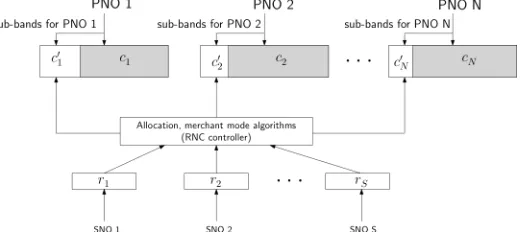
We consider a cellular network to consists of S secondary network operators (SNOs) and N,
with size |N |= N, denote the set of primary network operators (PNOs) serving a region R, see Figure 1. Let L, with size |L | = L, be the set of cells in the region.
Eachprimary and secondary operatorin the network is licensed with an incumbent bandwidth
consisting of a set of component carriers, each of which can be allocated to support the operators’
subscribers. The antenna towers/masts at the centre of each cell i ∈ L is shared among the
operators. The operators are managed by radio network controllers (RNC) which monitor base
stations and assign resources for the air interface as well as other functions [31, 32]. In the
context of this cellular networks arrangement, we only consider cells with an almost identical
radio environment, which is visible to all providers in each cell. An example of this setup is
when a town or city requires operators to use common towers for their antennas, due to economy
of scale property of telecommunication industry.
Due to spectrum liberalisation, the PNOs |N | will have the freedom to lease their spectrum
bandwidths to the SNOs. Leasing spectrum bandwidths would mean that the SNO will have to
pay a certain compensation to the PNO for using the spectrum bandwidths, and the amount of
compensation is expected to be proportional to the amount of allowed spectrum leasing by the
primary system. We assume the compensation paid to the PNO is in form of monetary value. The
PNOs broadcast specific information about their available bands for leasing and admission cost
(per unit bandwidth) at each celli ∈ L at fixed identical intervals (e.g., every 2 hours). The lease conditions may specify additional parameters such as the extent of spatial region for spectrum
the spectrum to the PNO at the end of the lease interval. The duration of each lease could be
decided by the network providers under a mutual agreement, and/or any other regulatory bodies’
conditions (e.g., minutes, hours, days). In our model, we assume that the PNOs receive a series
of demands from multiple SNOs at different time instances [25, 33]. Depending on the time of
SNO’s request, different sets of frequencies and prices can be available. Demands are awarded
instantaneously, in which case the borrowed spectrum can be immediately used. We consider
the spectrum sharing problem among multiple SNOs, which support different types of spectrum
bands and hence have heterogeneous GoS demands at different cells.
The available channels may vary in the bandwidth and transmitting range to support different
sizes of cells and cells with different terrain characteristics. The connectivity and scalability of
the network varies because a channel with shorter transmission range may not cover all the areas
covered by a channel with a longer transmission range. Thus, there is an obvious need for further
band’s categorisation prior to spectrum trading, which takes heterogeneity of cells into account.
We address this issue by considering multiple types of spectrum bands, assuming that each have
different characteristics (e.g., 800 MHz, 1.8 GHz and 2.5 GHz bands). This will be useful when
[image:6.612.183.443.426.544.2]considering 5G networks where a variety of bands are expected to be in deployment.
Fig. 1: Network model for cellular network with N PNOs and S SNOs
III. PROBLEM FORMULATION
Considering the system model described in Section II, the problem now becomes how the
RNC of an SNO acquires additional spectrum from the PNOs. The spectrum borrowing can be
performed by considering one of the following objectives:
• to minimize borrowing cost in each time slot by selecting the lowest cost combinations of
• to maximize profit in each time slot by borrowing the highest profit combinations of available
spectrum from the primary networks under restricted budget to achieve a specified GoS.
In principle, the RNC’s objective is to minimize overall operating cost or to maximize revenue
for an SNO as well as to maximize utility to the end users.
A. Modelling assumptions
In this subsection we identify the part of network information which is assumed to be known
to the SNOs:
• arrival rate of the sth SNO at ith cell for jth type of spectrum band λsij, ∀s,i, j, • service rate of the sth SNO at ith cell for jth type of spectrum band µsij, ∀s,i, j,
• available bandwidth of the sth SNO at ith cell for jth type of spectrum band wsij, ∀s,i, j, • borrowing cost of the sth SNO for unit bandwidth from the PNOs atith cell for jth type of
spectrum bandcijk, ∀i, j,k (which are assumed to be announced periodically by the PNOs),
• allocated budget for borrowing bandwidths to thesth SNO atith cell for jth type of spectrum
bandfrom the PNOs bsij, ∀s,i, j,
• available bandwidth of the kth PNO at ith cell for jth type of spectrum band aijk, ∀i, j,k,
(which are assumed to be announced periodically by the PNOs), and
Time is divided into equal-length slots T = {0,1,2, . . .}. At each time slot t ∈ T the process of aggregated channel borrowing is repeated. We use the time indicator (t) to emphasise the vectors dependancy in time. Trading of bandwidth is done between primary and secondary providers
separately in each of successive time windows of a particular duration. Henceforth, we focus on
the the process of channel borrowing and optimization in a single window.
B. Notations used in Problem 1 and Problem 2
Let us define the following quantities which are used later in mathematical programming
problems (Problem 1 and Problem 2):
cijk(t) B cost of unit bandwidth to be borrowed from kth PNO for j type resource atith cell
during time interval t, where cijk(t) ∈ R L×Ni j
≥0
cijk(t) > 0
and Nij is the number of PNOs in
xijk(t) B unit of spectrum bandwidths (or sub-bands) to be borrowed from kth PNO for j
type resource at ith cell during time interval t, where xijk(t) ∈R L×Ni j
≥0 .
θijk(t) B PNOs intrinsic quality (e.g., the extent of the coverage area and/or maximum
allowable transmit power), where {θij1, θij2, . . . , θijk, . . . , θL×N}.
psij(t) B target blocking probability for j type resource at ith cell during time interval t for
the secondary network operator.
aijk(t) Bunit bandwidth available fromkth PNO to be leased tosth SNO for jth type resource
at the ith cell during time interval t, where aijk(t) ∈R L×Ni j
≥0 .
rsij(t) B unit bandwidth required to satisfy the target blocking probability pij(t) for the sth
SNO’s for jth type resource at ith cell during time interval t, whererij(t) ∈R L
≥0.
γijk(t) Bthe expected profit for borrowing unit bandwidth fromkth PNO for jth type resource
at ith cell during time interval t, where γijk(t) ∈R L×Ni j
.
C. Spectrum allocation by minimising borrowing cost
We now formulate the spectrum allocation problem, that is, how much spectrum bandwidths
to be borrowed from each PNO to keep the blocking probability in a specific level, for instance,
at 1%. Given a set of possible available spectrum resources {aijk(t)} and their associated prices
{cijk(t)}, the problem is to find the feasible set of spectrum bandwidths {xijk(t)} by minimising
the total borrowing cost. The PNOs set their prices according to the maximum allowed transmit
power $ijk and the pricing coefficient ϕijk, which can be expressed as [9]
cijk =
* . .
, X
k∈ai j k
"
log 1+ h$ijk
%i
!
−($ijk ·ϕijk)
# + / /
-·(aijk)
−1 (1)
where h is the average aggregated channel gain, %i is the additive noise received by SNO users
at celli and ϕijk represents pricing coefficient of PNO k for the SNO in the ith cell for causing
each unit of interference. Equation (1) shows that PNOs select prices in a way such that the
collective preference order of transmit power, channel gain and noise are retained. This cancels
the intuition that prices are selected so that all channels available for borrowing are equally
its channel to the SNOs and therefore it is not possible to select a price lower than X(min) such
that
cijk =
RHS of Eq. (1), RHS of Eq. (1)≥ X(min)
X(min), otherwise.
(2)
Resource acquisition in this case for the sth SNO is obtained by solving the following
optimization problem: Problem 1: minimize L X
ij=1 Ni j
X
k=1
cijk(t) · xijk(t)· θijk(t)
, (3) subject to arg min
xi j k∀i,j,k
Prλsij(t), µsij(t), ωsij
≤ psij(t), ∀ij,k (4)
xijk(t) ≤ aijk(t), ∀ij,k (5) Ni j
X
k=1
xijk(t) ≤ rsij(t), ∀ij,k (6)
whereωsij =
PNi j
k=1xijk(t)+wsij is the total bandwidth (available and borrowed bandwidth from
the PNOs).
In contrast to the formulation of Problem 1, borrowing cost for each cell i can be calculated as PNi j
k=1cijk(t) · xijk(t)· θijk(t). The parameter θijk(t) (0 ≤ θijk(t) ≤ 1) defines the intrinsic
quality by weighing the cost of borrowing spectrum bandwidths. The intrinsic quality represents
the quality of the available heterogeneous aggregated channels to carry the data for transmission.
Therefore, the price per unit bandwidth in each PNO can vary, i.e.,cijk(t) Q cijl(t),∀ij and∀k,l
with k , l. We thus refer to this pricing scheme as non-uniform pricing.
The constraint (4) in Problem 1 guarantees that the sth SNO is borrowing enough to fulfil
its demand. The blocking probability in constraint (4) is a non-linear function of spectrum
bandwidth for each cell. Therefore, the above optimization problem is considered as a
non-linear optimization, which can be solved in two phases, In the first phase the SNOs set the
target blocking probability for each cell (e.g., psij = 0.01, ∀ij). Then SNOs calculates the
bandwidthrsij(t) required to achieve the target blocking probability psij(t) for each celli. Next
that the channel request rates and service rates follow Markov processes (i.e., inter-arrival and
service times are exponential) for all PNOs and SNOs. A channel request is immediately lost if
it finds the system busy, which implies that networks operate independently in a non-cooperative
way. This is referred to as an Erlang loss system [25, 34]. Under a loss system the well-known
blocking probability for the jth type of service at the ith cell of the sth SNO can be given by
the Erlang B formula as
psij(t) =
1 wsij!
λsij(t)
µsij(t) !wsi j
wsi j X
n=0
1 n!
λsij(t)
µsij(t) !n
−1
. (7)
where λsij(t), µsij(t) andwsij are arrival rate, service rate and existing capacity of the sth SNO,
respectively. Note that during the post-optimization analysis new blocking probability formula
are developed to accommodate sharing and interaction between operators in Section III-G.
Now with the existing bandwidth wsij, we first calculate the total required bandwidth τsij(t)
to achieve the target blocking probability for the ith cell of the SNO
τsij(t) = f
−1
Prλsij(t), µsij(t),wsij . (8)
where f−1(·) is the inverse function of P(b)(t) (equation 7) used to derive the required capacity
over the existing capacity. As the function is non-linear in λsij(t), µsij(t) and τsij(t), it is not
easy to get an explicit expression for τsij(t) for a given target blocking probability. However, it
is possible to calculate τsij(t) iteratively for given values of λsij(t), µsij(t) and a target blocking
probability psij(t). Subtracting the existing bandwidth wsij from the total required τsij(t), we
obtain the required bandwidth rsij(t) at the ith cell of the SNO during time intervalt
rsij(t) = τsij(t)−wsij. (9)
Now the problem is to find the feasible set of bandwidth xijk(t) from the PNOs which
minimizes the borrowing cost. This is done in the next mathematical programming phase (see
Algorithm 1 for details).
In the second phase, we set up the borrowing costcijk(t) and the maximum possible bandwidth
available aijk(t). The borrowing decisions of the sth SNO are made subject to the lowest price
a number of acquisitions, e.g., the sth SNO selects the lowest price from the available set of bandwidths from the PNOs. If the acquired resources aijk(t) are insufficient to reach the target
blocking probability psij(t) (i.e.,rsijk(t)−aijk(t) > 0), then the SNO borrows from the remaining
bandwidths from the set {aij1(t),aij2(t), . . . ,aijN(t)}=aijk(t) for which the cost is minimum. If
the required blocking probability pij(t) is reached, then the SNO stops acquiring new spectrum
bandwidths until the next time interval (t+1).
Once the problem is solved, the new blocking probability for the sth SNO can be calculated as
P(bnew
si j)(t)= Pr
* .
,
λsij(t), µsij(t),*. ,
wsij + Ni j
X
k=1
xijk(t)+/ -+ /
-= ω1
sij!
λsij(t)
µsij(t)
!ωsi j
ωsi j
X
n=0
1
n!
λsij(t)
µsij(t)
!n −1 , (10) where
ωsij = wsij + Ni j
X
k=1
xijk(t). (11)
Consequently, the sth SNO will achieve the blocking probability with the required amount of bandwidths satisfying the target blocking probabilitypsij(t) or with the highest possible borrowed
bandwidths which is mathematically expressed as
P(bnew si j)(t)=
psij(t),
PNi j
k=1aijk(t) ≥rsij(t)
P(bnew
si j)(t), otherwise.
(12)
Algorithm 1: Optimal spectrum borrowing.
1 Calculate rij∀i,j which satisfies pij, and get cijk and aijk ∀i, j,k.
2 for every time slot (t) do
3 for all cells i ←1 : L do
4 for PNOs k =1 : N do
5 Solve the nonlinear stochastic Problem 1 s.t. constraints (4), (5) and (6).
D. Spectrum allocation using heuristic algorithm
In this approach, spectrum acquisition is performed randomly as illustrated in Algorithm 2.
The optimal borrowing cost using this algorithm can only be found randomly from the set of
capacity values {aijk} by satisfying the constraints in equation (5) and (6).
Algorithm 2: Heuristic spectrum borrowing.
1 Calculate rij∀i,j which satisfies pij, and get cijk and aijk ∀i, j,k.
2 for every time slot (t) do
3 for all cells i ←1 : L do
4 Set xijk ← {φ}, where {φ} is an empty set.
5 Set counter←Pk xijk.
6 Choose a random integer n ∈ {1,2, . . . ,N}. 7 for all PNOs k = n: N 1 : (n−1) do 8 if 0< aijk > (rij −counter) then
9 xijk ← (rij −counter).
10 break
11 else if aijk > 0 & (counter < rij) then
12 xijk ← aijk.
13 counter←counter+xijk.
14 else
15 xijk ← 0.
16 return Total borrowing cost
For all i, j and k, equation (6) ensures that the sth SNO does not borrow more than the
network’s bandwidths demand by controlling the borrowed spectrum bandwidth size in each
iteration, which can be expressed mathematically as
xijk(t) =
aijk(t), rij(t) ≥ aijk(t)
rsij(t), otherwise.
(13)
This scenario can also be regarded as round-robin scheduling algorithm, where SNOs randomly
gain access to the PNOs’ available spectrum, and the PNOs serve one SNO in each turn. The
resource allocation in algorithm 2 evolves in two main discrete steps:
The only difference between the two formulations is that in the heuristic formulation, the cost
of spectrum access is not considered, where spectrum acquisition is performed randomly from
the set {aijk}. Note that when
P
aijk ≤ rsij the feasible set {xijk} is equal for both formulations.
We also note that when PNi j
k=1aijk(t) >rsij(t), the optimal and heuristic algorithm may achieve
the same outcome in terms of total borrowing cost, however, this is a result of randomness in
the selection process with probability
P(selecting optimal bandwidths) =
1
N aijk ≥ rsij,∀ij
1
{a¯ij..}
P
m{a¯ijlm, ∀l,m} ≥rsij,∀ij
1 PNi j
k=1aijk ≤rsij,∀ij
(14)
where {a¯ijlm, ∀l,m} ⊂ {aijk,∀ij,k}, and
{a¯ij..}
is the number of subsets in the set {a¯ij..} which
satisfy the bandwidth requirement for the ith cell with jth type of spectrum band.
Remark 1. In Problem 1, the objective function and all constraints are linear except for the
constraint (4). Once we calculate the required bandwidth for the ith cell using the non-linear
constraint (4) iteratively we then solve the optimization Problem 1 using Algorithm 1. With
the remaining of the constraints the optimization problem is solved by the well-known revised
simplex method. However, the computational complexity in Algorithm 1 is polynomial time,
i.e. O(n) time. The computational time increases linearly with number of cells and number of
PNOs. The heuristic counterpart, Algorithm 2, arbitrarily borrows bandwidths from the PNOs
until the target blocking probability of the SNO is achieved. Since the algorithm finds a solution
by performing a combinatorics satisfying a set of constraints, the computational complexity is
quadratic time, i.e. O(n2)with number of PNOs (N ) and exponential time, i.e.2nwith number of
cells (L). Note that the Algorithm 2 does not guarantee the optimal solution and the probability
of finding an optimal solution by the heuristic algorithm is given in equation (14).
E. Expected profit maximization under restricted budget
In this section, we formulate the second spectrum allocation problem that illustrates how
a specific level. Given a set of possible available spectrum resources {aijk(t)}, their associated
prices {cijk(t)} and expected profit {γijk(t)}, the problem is to find the feasible set of spectrum
bandwidths {xijk(t)} by maximising the total profit of the sth SNO, under allocated budget and
performing the selection process according to the highest possible profit combination. Resource
acquisition in this case is obtained by solving the following optimization problem:
Problem 2: maximize L X
i=1
M
X
j=1
Nj
X
k=1
γijk(t) · xijk(t)
(15) subject to arg min
xi j k∀i,j,k
Prλsij(t), µsij(t), ωsij
≤ psij(t), ∀ij,k (16)
xijk(t) ≤ aijk(t),∀ij,k (17) Ni j
X
k=1
xijk(t) ≤ rsij(t), ∀ij,k (18) Nj
X
k=1
cijk(t) · xijk(t) ≤ bsij, ∀s,ij,k, (19)
where γijk(t) consists of two parts: the expected revenue vij(t) and cost cijk(t), which can be
obtained as
γijk(t) =vijk(t)−cijk(t), (20)
Here
vijk(t)= f
βij(t), θijk(t)
. (21)
where βij(t) is the selling price per unit bandwidth for the ith cell and jth type service during
time period t. In equation (21), the expected revenue vijk(t) is the function f(·) of the selling
price βijk(t) and the intrinsic quality (θijk(t)) which may take, in general, a non-linear form. In
the simplest case, the function can be defined as
vijk(t) = βijk(t)
f
−e−θi j k(t)g. (22)
We consider the the intrinsic quality per unit bandwidth (θijk(t)) for each PNO, which can vary,
i.e., θijk(t) Q θijl(t), ∀ij and∀k,l with k ,l according to spatial structure of the base stations,
θijk(t) influences the optimal spectrum borrowing decisions.
The revenue earned through the sale of the borrowed bandwidth can be equal, higher or lower
than the cost. However, for simplicity, we model the revenue vijk(t) earned through the sale of
the borrowed bandwidth to exceed the borrowing cost, i.e.,vijk(t) > cijk(t) due to the assumption
that profit of the sth SNO for borrowing a unit bandwidth is always positive (γijk(t)).
The inequality constraint in equation (19) implies that the sth SNO maximizes its profit by taking into account the limitations imposed by cost of the utility and the maximum allowable
expenditure which the sth SNO can spend for borrowing spectrum demand in each cell. Next,
we solve the the above non-linear optimization problem in two phases:
In the first phase, the same steps are performed using equation (16) as for solving Problem 1.
Thesth SNO calculates the spectrum demand to meet its time varying target blocking probability over time and location. The spectrum demand is adjusted dynamically based on the network
information provided by the expected cell demand, service rate and existing spectrum bandwidth.
In the second phase, we set up the vectors {cijk(t)}, {aijk(t)} and {γijk(t)}. The borrowing
decisions of the sth SNO are made subject to achieving the maximum profit for each acquisition from the PNOs. In Problem 1, the budget restriction is not considered, where the sth SNO is allowed to make spectrum bandwidth borrowing until it meets the spectrum demand, i.e.,
Nj
X
k=1
xijk(t) =rsij(t), assuming Nj
X
k=1
aijk(t) ≥ rsij(t). (23)
Algorithm 3: Optimal spectrum borrowing under restricted budget.
1 Calculate rij ∀i,j which satisfies pij, and get cijk, aijk, γijk and θijk(t) ∀i, j,k.
2 Set maximum allowed budget expenditure for every cell bij. 3 for every time slot (t) do
4 for all cells i ←1 : L do
5 for all PNOs k =1 : N do
6 Solve the nonlinear stochastic Problem 2 s.t. (16), (17), (18) and (19).
7 return Total profit
However, in this formulation, the borrowing capacity of each SNO is restricted to budget
GoS, then Problem 2 is infeasible. The SNOs only achieves a best effort service to minimize the blocking probability so far as the budget permits.
Algorithm 4: Heuristic spectrum borrowing under restricted budget.
1 Calculate rij ∀i,j which satisfies pij, and get cijk, aijk, γijk and θijk(t) ∀i, j,k.
2 Set maximum allowed budget expenditure for every cell bij.
3 for every time slot (t) do
4 for all cells i ←1 : L do
5 Set xijk ← {φ}, where {φ} is an empty set.
6 Set counter←Pk xijk.
7 Choose a random integer n ∈ {1,2, . . . ,N}. 8 for all PNOs k = n: N and 1 : (n−1) do
9 if (0 < aijk) ≤ (rij - counter) & (cijk ∗aijk) ≤ bij then
10 xijk ← aijk.
11 counter←counter+Pxijk.
12 bij ← bij −
P
(xijk ∗cijk).
13 else if (aijk > 0) & cijk ≤ (bij −counter) & (aijk∗cijk) ≥ bij then 14 xijk ←
$
bij
cijk
%
where bxc means the floor of x.
15 counter←counter+Pxijk.
16 bij ← bij −
P
xijk.∗cijk.
17 else if counter≤ rij & aijk >0 & aijk ≥ (rij−counter) & (aijk∗cijk) ≤ bij then
18 xijk ←rij −counter.
19 counter←counter+Pxijk.
20 bij ← bij −
P
xijk.∗cijk.
21 break
22 else if counter≤ rij & aijk >0 & aijk ≥ (rij−counter) & (aijk∗cijk) ≥ bij then
23 xijk ← min
($b
ij
cijk
%)
.
24 counter←counter+Pxijk.
25 bij ← bij −
P
xijk∗cijk.
26 else
27 xijk ← 0.
28 return Total profit
F. Spectrum allocation using heuristic algorithm under budget constraint
In this subsection, we solve the problem of spectrum allocation under budget constraint by
as in Algorithm 3. However, Algorithm 4 does not perform spectrum selection according to
the highest possible profit combination from the set {aijk}, rather runs on randomly selected
combination from the set {aijk} to satisfy the spectrum demand rsij. The optimal profit using
Algorithm 4 can only be found from the set of capacity values {aijk} satisfying the constraints
in equation (17), (18) and (19) with probability given in equation (14). To satisfy the constraints
in equation (17), (18) and (19) we use
xijk(t)=
aijk(t), rsij(t) ≥ aijk(t), bsij ≥ cijk,
rsij(t), rsij(t) < aijk(t), bsij ≥ cijk,
0, bsij < cijk orrsij(t) = 0.
(24)
Remark 2. Like Problem 1, in Problem 2 we have the non-linear constraint which is solved
iteratively and then the whole problem is solved by the revised simplex method. Therefore,
Algorithm 3 is polynomial time and the heuristic counterpart (Algorithm 4) is again quadratic
time/exponential time depending on number of cells and PNOs.
G. Post-optimization analysis under resource sharing between SNOs and PNOs
In the optimization problems above, the PNOs lease part of their spectrum resources to SNOs
for monetary benefits. The leasing and borrowing was based on fixed arrival rate and available
spectrum resources. However, the demand in the PNOs may be bursty during trading window
causing one or more of PNOs’ state to change from the underloaded to overloaded and their
blocking probability would increase. As a consequence, a PNO may react by deviating part or all
of its leased spectrum resources under mutual agreement, which results in reducing the size of the
shared spectrum resources. This dynamic mechanism affects the performance of all operators
involved in the trading. The complexity of the problem depends primarily on the number of
PNOs and SNOs involved and the level of interactions between them.
In this paper, we present an analytical methodology to model and analyze the above
Consider a cell consisting of S SNOs with capacitycs1,cs2, . . . ,css and N PNOs with capacity
c1,c2, . . . ,cN, respectively. Under a sharing agreement all N PNOs share part of their resources
c01,c02, . . . ,c0N, respectively with S SNOs determined using the optimization approach discussed
in the previous sections. These resources may also be used by the corresponding PNO under
mutual agreement. A state of the network is a vector of length [S(1+N)+2N)] defined as
n= {(ns1,ns2, . . . ,nss); ((ns11,ns12, . . . ,ns1n), . . . ,(nsS1,nsS2, . . . ,nsSn));
(n1,n2, . . . ,nN); (n11,n22, . . . ,nN N)}
with the condition that (ns1i,ns2i, . . . ,nsSi)+nii ≤ c
0
i ∀ i = 1,2, . . . ,N, where nsi is the number
of channel requests in progress in the ith SNO; nsij is the number of channel requests in the
shared resources of the ith PNO from the sith SNO; nj is the number of channel requests in
progress in the jth PNO and nj j is the number of request of the jth PNO on its own shared
resources. The states n are restricted due to resource sharing constraints. The set of feasible
states can be written as
Ωs = {n:An≤ s} (25)
whereA is a [S(1+N)+2N)] matrix and s is ad-vector, where d is the number of constraints.
The network topology is reflected in the matrix A and the vector s.
Let channel requests arrive to theith secondary and jth primary operators according to a
non-homogeneous Poisson process, with rates λsi(t) and λj(t) at time t. These requests are admitted
if n+ei ∈ Ωs (if PNO) and n+ej ∈ Ωs (if SNO), where ei and ej is the ith unit vector with
1 in place i and 0 elsewhere. When all csi resources of the ith SNO is full then requests are
diverted and admitted to the jth PNO ifn+ei j ∈Ωs, where ei j is theith unit vector. Similarly, in
the jth PNO being all cj resources occupied requests are diverted to its shared resources c0j for
the jth primary network if n+ej j ∈Ωs, where ej j is the ith unit vector. Assume that admitted
requests in ith secondary and jth primary operators have exponential holding times with rates
µsi(t) and µj(t) respectively at time t. Under these assumptions, the network can be modeled
as a non-homogeneous continuous time Markov chain
X(t) = (Xi(t),Xi j(t),Xj j(t),Xj(t); i= 1,2, . . . ,S,j =1,2, . . . ,N, t ≥ 0) (26)
the Markov chain is specified in (25), and its transition rates Q(t) = (q(n,n0,t),n,n0 ∈ Ωs) are
given by
q(n,n0,t) =
λsi(t) n
0=n+e
i or n0=n+ei j, if nsi =csi, i= 1,2, . . . ,S
λj(t) n0=n+ej or n0=n+ej j, if nj =cj, j =1,2, . . . ,N
nsiµsi(t) n
0=n−e
i, i =1,2, . . . ,S
njµj(t) n0=n−ej, j =1,2, . . . ,N
nsijµsi(t) n
0=n−e
i j, i =1,2, . . . ,S, j =1,2, . . . ,N
nj jµj(t) n0=n−ej j, j =1,2, . . . ,N
(27)
Theorem 1. The closed-form solution of n channel requests in progress at time t is given by
equation (28).
P(n,t)= K−1
ρ(ns1+ns11+···+ns1N)
s1 (t)
· · ·
ρ(nsS+nsS1+···+nsS N)
sS (t)
(ns1+ns11+· · ·+ns1N)! · · · (ns1 +ns11+· · ·+ns1N)!
·
f
ρ(n1+n11)
1 (t)
g
· fρ(n2+n22)
2 (t)
g
· · ·fρ(nN+nN N)
N (t)
g
(n1+n11)! (n2+n22)! · · · (nN +nN N)!
∀ n∈Ωs (28)
where ρsi = λsi/µsi and ρj = λj/µj are traffic intensities of the sith SNO and jth PNO,
respectively and K is the normalizing constant and given by
K = X
n∈Ωs
ρ(ns1+ns11+···+ns1N)
s1 (t)
· · ·
ρ(nsS+nsS1+···+nsS N)
sS (t)
(ns1 +ns11+· · ·+ns1N)! · · · (ns1+ns11+· · ·+ns1N)!
·
f
ρ(n1+n11)
1 (t)
g
· fρ(n2+n22)
2 (t)
g
· · ·fρ(nN+nN N)
N (t)
g
(n1+n11)! (n2+n22)! · · · (nN +nN N)!
∀ n∈Ωs. (29)
Proof. Define the state probabilities
P(n,t) := Pr(X(t) =n), n∈Ωs, t ≥ 0 (30)
with initial condition P0(n) = Pr(X(0) = n). Since the network has a finite state space, these
probabilities are the unique solution of the Kolmogorov forward equations given in (31) for
The Kolmogorov forward equations can be defined as
dP(n,t)
dt =
" S X
i=1
λsi(t)·
1(nsi < csi)+1(nsi = csi ∩n+ei j)
+
N
X
j=1
λj(t)· 1(nj < cj)
+1(nj =cj ∩n−ej j)
#
·P((n−ei),t)+ S
X
i=1
(nsi +1)µsi(t)P((n+ei),t)
+
N
X
j=1
(nj +1)µj(t)·P((n+ej),t)−
" S X
i=1
λsi(t)·
1(nsi < csi)+1(nsi = csi ∩n+ei j)
+
N
X
j=1
λj(t)· 1(nj < cj)+1(nj = cj∩n−ej j)+ S
X
i=1
nsiµsi(t)+
N
X
j=1
njµj(t)
#
P(n,t)
(31)
where 1(A) is the indicator function for an event A.
Equations in (31) can be written in the operator form as given by
dP(t)
dt =P(t)Q(t), P(0)= P0, t > 0 (32)
where P(t) is the vector of probabilities P(n,t). The formal solution of the equation (32) is
given by
P(t)= P0EQ(t), t ≥ 0 (33)
where EQ(t) is the time-ordered exponential of the generator Q(t), that is the unique operator
solution to the equation
dEQ(t)
dt = EQ(0)Q(t), t ≥ 0 (34)
whereEQ(0)= I, the identity operator. The unique solution of the Kolmogorov forward equations
(31) is then given by the equation (28).
The blocking probability formula can then be derived from the closed-form solution (28). The
blocking probability for an operator i (ith operator could be an SNO or a PNO), is then given
by
Pb(t) =
X
n∈S
=
P
n∈S
"
ρ(ns1+ns11+···+ns1N)
s1 (t)
#
···
"
ρ(nsS+nsS1+···+nsS N)
sS (t)
#
·
ρ(n1+n11 ) 1 (t)
···
ρ(n N+n N N) N (t)
(ns1+ns11+···+ns1N)!···(ns1+ns11+···+ns1N)!(n1+n11)!···(nN+nN N)!
P
n∈Ωs
"
ρ(ns1+ns11+···+ns1N)
s1 (t)
#
···
"
ρ(nsS+nsS1+···+nsS N)
sS (t)
#
·
ρ(n1+n11 ) 1 (t)
···
ρ(n N+n N N) N (t)
(ns1+ns11+···+ns1N)!···(ns1+ns11+···+ns1N)!(n1+n11)!···(nN+nN N)!
(36)
where the set S is the restricted state space, and varies for the SNOs and PNOs. For the sth
SNO, it is defined as
Si = n∈Ωs|(nsi =csi∩nsi1+n11= c
0
1∩nsi2+n22 = c
0
2∩· · ·∩nsiN+nN N =c
0
N) , i= 1,2, . . . ,S.
(37)
and for the jth PNO, Si can be replaced by Sj and defined as
Si = n∈Ωs|(nsi =csi ∩nsij+nj j =c
0
i) , j =1,2, . . . ,N. (38)
IV. RESULTS AND ANALYSIS
In this section, we show the analysis of optimal borrowing solutions by Algorithms 1 and 3
corresponding to the cost minimization and profit maximization with restricted budget scenarios,
respectively. To explore the advantages of the proposed formulations, we compare the results
from Algorithm 1 and 3 with a heuristic spectrum selection formulation by Algorithm 2 and 4,
respectively. We simulate the functionalities of the network management, which are necessary to
generate the optimal solution and to compare with the heuristic spectrum selection algorithms.
We consider one SNO and four PNOs (N = 4) to simulate the dynamics of the merchant mode
resource sharing mechanism. Some parameters are determined randomly by the algorithms with
[image:21.612.71.540.605.666.2]specific distribution (e.g., λi, µi, wi) while other parameters are preset (e.g., L, pij).
TABLE I: Simulation parameters.
Parameter L M N pij λij µij wij cijk aijk bij
Values forproblem 1 100 1 4 0.01 10 1 1 (3,9) (5,10) −−
A. Cost analysis under target performance (Problem 1)
In the simulation, we consider the PNOs spectral usage for all cellsL, where four base stations of primary network operators in each cell are deployed (collocated topology), e.g., the case in
densely populated cities. The demand of service for each provider (primary or secondary) vary
over time and location. We assume the spectral utilisation of secondary provider at time interval
t is high whereas the PNOs are underloaded in the same time interval and at the same location.
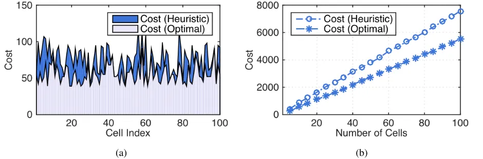
[image:22.612.71.541.215.370.2](a) (b)
Fig. 2: Cost with optimal and heuristic algorithms for (a) per cell and (b) for varying number of cells.
The PNOs charge the SNO at variable rates. The charges may be assessed by the market on
the basis of the current supply-demand balance for each individual operator at each cell and
possibly other factors [12]. However, we set limits to the price of unit bandwidth as maximum
X(max) and minimum price X(min) to structure the problem space. For the purpose of analysis, we parametrise the borrowing cost as cijk(t) =
(
cijk(t) | X(min) ≤ cijk(t) ≤ X(max)
)
, where cijk(t)
follows a uniform distribution from [X(min) = 3, X(max) = 9]. We keep the difference between
X(max) and X(min) relatively small at all cells. This assumption captures the highly competitive nature of the market economic environment. We determine the admission cost per unit bandwidth
based on a discrete uniform random variables. In our mathematical model all possible variations
of the available bandwidth values aijk(t) to provide the SNO demand are considered. This
assumption provides realistic scenarios where PNOs could have different values of leasable
spectrum resources. More details about the simulation parameters are given in Table I.
considering the SNO’s expected traffic load λij in the next time interval, the available capacity
wij and service rate µij, each cell determines its required number of channels rij(t).
For comparisons, we simulate the interactions between the network providers and we solve the
resource allocation problem by the optimal and the heuristic allocation as described in Algorithms
1 and 2, respectively. For the simulation of the heuristic allocation, each cell i makes heuristic selection of aggregated channels for dynamic access from the set {aijk} which are collocated in
the same cell. The selection of aggregated channels is performed regardless of the admission
cost associated with the choice of selected channels. Algorithm 2 is allowed to perform spectrum
borrowing until the demand is satisfied, assuming PNi j
k=1aijk(t) ≥ rij(t). If
PNi j
k=1aijk(t) < rij(t)
then the algorithm takes all available bandwidths, however, the target blocking probability will
not be satisfied, such that, P(bnew)(t) < pij(t).
For the Algorithm 1, the cells of SNO select the combination {xijk} with the lowest admission
cost from the set {aijk(t)}, ∀k,i, to achieve the optimal channel borrowing admission costs. It
is possible that there may be multiple solutions for the allocation problem which provide the
same required bandwidth to the SNO with different costs.
The main observation here is that the optimal model achieves lower costs compared to the
heuristic algorithm, except for cells with PNi j
k=1aijk(t) <rij(t), see Figure 2a. It is also observed
that the total borrowing cost of both the heuristic and optimal configuration vary in every cell
due to the stochastic nature of the costs and number of available channels.
If we consider the admission cost for large number of cells, as we can see from Figure 2b,
we notice that as the number of cells increase, the difference in cost between the heuristic and
the optimal selection algorithm becomes larger, which implies substantial savings for operators
with large territories when the optimal algorithm is used.
We also investigate the effect of target blocking probability on the admission cost. In Figure
3 we show the results for different target blocking probabilities ranging from 0−0.9 for a single cell. We clearly see that as pij →0, the admission cost increases for both algorithms. However,
the optimal algorithm (Algorithm 1) provides lower borrowing cost for most of the points.
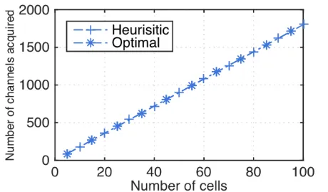
The total number of aggregated channels which are acquired through borrowing by using
Algorithms 1 and 2 is equal, see Figure 4. This is because both algorithms allow channels to
Fig. 3: Effect of varying target blocking probability on cost for optimal and heuristic algorithms.
Fig. 4: Effect of borrowing on bandwidth acquisition for the optimal and heuristic al-gorithms.
of PNOs {aijk} are consumed.
B. Expected profit analysis under budget constraints (Problem 2)
The objective of the secondary providers can be described from both economic and system
performance perspective. Firstly, the SNO aims to lower the blocking probability for its
sub-scribers. Secondly, the SNO attempts to maximize its profit by leasing additional spectrum from
the PNOs in terms of cost and intrinsic quality. However, since network operators often operate
with limited budget, SNO can only spend bij(t) amount of resources/money at a cell i and time
interval t. This is imposed by the government and regulatory bodies to keep the fairness of
spectrum leasing among network operators.
To demonstrate the gain of Algorithm 3, detailed investigation has been made and the results
are compared with Algorithm 4. Figure 5a shows the optimal algorithm can achieve substantial
gain in comparison to the heuristic allocation approach. However, both algorithms provide
acceptable efficiency in terms of GoS. We also notice that as the number of cells increase
the profit of the SNO gets larger, see Figure 5b.
Figure 6 shows the effect of budget and target blocking probability on achievable profit with
varying budget expenditure between 0−250 and target blocking probability between 0 and 0.8 for a single cell. It is clear that as we increase the budget further bij →250, the profit increases
with respect to the increase of budget and demand. However, as the budget reaches a certain
(a) (b)
[image:25.612.73.538.64.221.2]Fig. 5: Profit using the optimal and heuristic algorithms for (a) per cell and (b) for varying number of cells.
[image:25.612.81.290.293.438.2]Fig. 6: Expected profit of the SNO for spec-trum borrowing with target blocking proba-bility =0 to 0.8 and budget = 0 to 250.
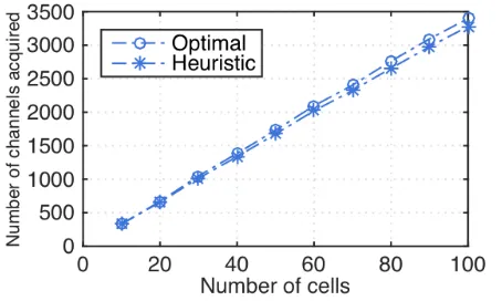
Fig. 7: Bandwidth acquisition of the SNO for spectrum borrowing by the optimal and heuristic algorithms.
We also study how the optimal allocation based on profit maximisation affects the amount of
acquired bandwidths. With number of cells between 1 and 100, we compare the two algorithms
presented to solve Problem 2, see Figure 7. We find that, the optimal algorithm can achieve
higher number of aggregated channels due to the higher efficiency in spectrum borrowing under
the restricted budget.
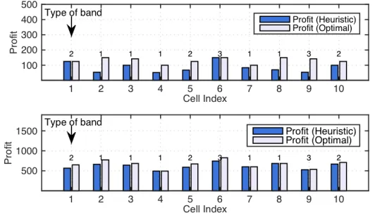
In the proposed algorithms, we added a functionality to allow the trading to be managed more
effectively by assigning each cell with a particular band type. In order to quantify the impact
of the proposed algorithms we simulated a network which could support three different bands,
[image:25.612.319.546.298.434.2]and allocated budget of 50 and 500 for each cell, we observed a markedly increased profit in
both cases, see Figure 8. We can also see from the figures (top and bottom figures) that in all
[image:26.612.172.438.148.301.2]types of bands, the optimal algorithm outperforms its heuristic counterpart.
Fig. 8: Effect of spectrum borrowing on profit with budget=50 (top) and budget= 500 (bottom).
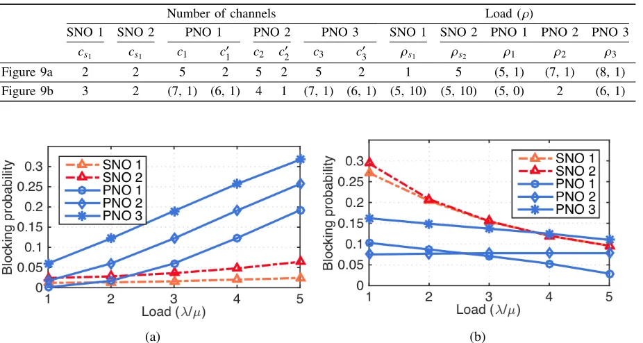
C. Post-optimization performance of the operators
To analyze the impact of unilateral deviation strategy of the PNOs, we used the closed form
formulae presented in Section III-G to compute the blocking probability of operators. The arrival
processes involved in all operators are non-homogenous Poisson with rates λs1, λs2, λ1, λ2, and
λ3, respectively. The offered loads are λs/µs and λi/µi for the sth secondary and ith PNO,
respectively. The number of aggregated channels and traffic intensities in each operator are
independent as shown in table II. The results show that the operators could obtain an actual
blocking probability values to determine their benefits when they engage in spectrum trading.
In Figure 9a, we observe the performance of the PNOs and the SNOs by varying the traffic
load at the PNOs (from 1 to 5). If we fix a particular value of traffic intensity at the SNOs
(ρs1 = 1 and ρs2 =5) and change it for the PNOs, then the SNOs’ blocking probability slightly
increase due to the available capacity for sharing (c01, c20 and c03) become overloaded by the
PNOs’ own traffic. We notice that the severity of traffic intensity change in the PNOs affects
the performance of the SNO.
In Figure 9b, we analyse the impact of change in state of the PNOs from overloaded to
underloaded. As the shared capacity becomes ample to meet the SNOs’ demand, we notice
TABLE II: Configurations used in Figure 9a and 9b.
Number of channels Load (ρ)
SNO 1 SNO 2 PNO 1 PNO 2 PNO 3 SNO 1 SNO 2 PNO 1 PNO 2 PNO 3
cs1 cs1 c1 c
0
1 c2 c 0
2 c3 c 0
[image:27.612.79.542.84.331.2]3 ρs1 ρs2 ρ1 ρ2 ρ3
Figure 9a 2 2 5 2 5 2 5 2 1 5 (5, 1) (7, 1) (8, 1)
Figure 9b 3 2 (7, 1) (6, 1) 4 1 (7, 1) (6, 1) (5, 10) (5, 10) (5, 0) 2 (6, 1)
(a) (b)
Fig. 9: Blocking probability for each operator when configuration details of (a) and (b) are according to Table II.
probability of PNO 2 is not affected by the changes in state of other primary and secondary
operators since its shared capacity and traffic load remains constant for the duration. The results
demonstrate that the derived blocking probabilities can provide a crucial insight to the sharing
strategies between operators.
V. CONCLUSION
In this paper, we presented two finite horizon nonlinear optimization algorithms to solve two
optimization problems for dynamic spectrum sharing. The efficiency of the proposed algorithms is
compared with their corresponding heuristic algorithms. We also presented the post-optimization
performance analysis of the SNO and PNOs through blocking probability, which provides useful
details about spectrum sharing strategy.
The optimization problems investigated by considering a comprehensive process of delivering
the SNO’s bandwidth demand and the solution algorithms ensured that either minimum cost of
bandwidth borrowing or maximum profit under budget restrictions are achieved depending on
spectrum from PNOs on temporal and spatial basis. Detailed comparisons are presented and they
showed that the gain in the results obtained from our proposed stochastic-optimization framework
is markedly higher than heuristic borrowing algorithms. Our proposed approaches facilitate a
dynamic purchasing (also called automation of licensing) scheme for such complex problems,
which provide incentives to the network operators wishing to adopt dynamic spectrum sharing
as well as substantial benefits for efficient use of spectrum. The proposed algorithms showed
significant opportunities to increase spectrum utilisation while keeping GoS at a particular level
and ensuring minimum cost. We also shown that our proposed optimization solution not only
reduce the total borrowing cost of the SNOs, but also finds maximum spectrum access under
any allocated budget.
A major challenge with the spectrum sharing optimization models is to guarantee the
oper-ational GoS under different sharing protocols. Although a vast amount of literature addressed
various spectrum sharing issues very little has discussed the post-optimization results which are
crucial for the operators to gain the detailed insight and final GoS. To study these issues and
provide the final GoS, we derived the blocking probability behavior using a time-dependent
continuous time Markov chain framework. Results showed that the final GoS is largely affected
by the increase of traffic at the PNOs and the amount of shared resources. This post-optimization
analysis of spectrum sharing among the operators is an emerging topic that requires further
re-search that would cover other issues, for instance, different sharing strategies and configurations.
REFERENCES
[1] A. Palaios, J. Riihijarvi, P. Mahonen, V. Atanasovski, L. Gavrilovska, P. Van Wesemael, A. Dejonghe, and P. Scheele,
“Two days of spectrum use in Europe,” in7th International Conference on Cognitive Radio Oriented Wireless Networks
and Communications, 2012, pp. 24–29.
[2] V. Valenta, R. Marˇs´alek, G. Baudoin, M. Villegas, M. Suarez, and F. Robert, “Survey on spectrum utilization in europe:
Measurements, analyses and observations,” in Fifth International Conference on Cognitive Radio Oriented Wireless
Networks and Communications, 2010, pp. 1–5.
[3] A. A. Khan, M. H. Rehmani, and M. Reisslein, “Cognitive radio for smart grids: Survey of architectures, spectrum sensing
mechanisms, and networking protocols,”IEEE Communications Surveys & Tutorials, vol. 18, no. 1, pp. 860–898, 2016.
[4] G. Ding, J. Wang, Q. Wu, Y.-D. Yao, F. Song, and T. A. Tsiftsis, “Cellular-base-station-assisted device-to-device
communications in tv white space,”IEEE J. Sel. Areas Commun., vol. 34, no. 1, pp. 107–121, 2016.
[6] H. Zhang, C. Jiang, X. Mao, and H.-H. Chen, “Interference-limited resource optimization in cognitive femtocells with
fairness and imperfect spectrum sensing,” IEEE Transactions on Vehicular Technology, vol. 65, no. 3, pp. 1761–1771,
2016.
[7] A. Afana, V. Asghari, A. Ghrayeb, and S. Affes, “On the performance of cooperative relaying spectrum-sharing systems
with collaborative distributed beamforming,”IEEE Transactions on Communications, vol. 62, no. 3, pp. 857–871, 2014.
[8] L. Wei, R. Q. Hu, Y. Qian, and G. Wu, “Energy efficiency and spectrum efficiency of multihop device-to-device
communications underlaying cellular networks,” IEEE Transactions on Vehicular Technology, vol. 65, no. 1, pp. 367–
380, 2016.
[9] Y. Xiao, Z. Han, C. Yuen, and L. A. DaSilva, “Carrier aggregation between operators in next generation cellular networks:
A stable roommate market,”IEEE Transactions on Wireless Communications, vol. 15, no. 1, pp. 633–650, 2016.
[10] R. Abozariba, M. Asaduzzaman, and M. Patwary, “Radio resource sharing framework for cooperative multi-operator
networks with dynamic overflow modelling,”IEEE Transactions on Vehicular Technology, 2016, In press.
[11] A. Ghosh and S. Sarkar, “Quality-sensitive price competition in secondary market spectrum oligopoly– single location
game,” IEEE/ACM Transactions on Networking, vol. 24, no. 3, pp. 1894–1907, 2016.
[12] G. Kasbekar, S. Sarkar, K. Kar, P. Muthuswamy, and A. Gupta, “Dynamic contract trading in spectrum markets,”IEEE
Transactions on Automatic Control, vol. 59, no. 10, pp. 2856–2862, 2014.
[13] M. Asaduzzaman, R. Abozariba, and M. Patwary, “Spectrum sharing optimization in cellular networks under target
performance and budget restriction,” in85th IEEE Vehicular Technology Conference, 2017.
[14] A. Ullah, S. Bhattarai, J.-M. Park, J. H. Reed, D. Gurney, and B. Bahrak, “Multi-tier exclusion zones for dynamic spectrum
sharing,” in2015 IEEE International Conference on Communications, 2015, pp. 7659–7664.
[15] Y. Zhang, C. Lee, D. Niyato, and P. Wang, “Auction approaches for resource allocation in wireless systems: A survey,”
IEEE Communications Surveys & Tutorials, vol. 15, no. 3, pp. 1020–1041, 2013.
[16] C. A. Gizelis and D. D. Vergados, “A survey of pricing schemes in wireless networks,”IEEE Communications Surveys &
Tutorials, vol. 13, no. 1, pp. 126–145, 2011.
[17] A.-H. Mohsenian-Rad, V. W. Wong, and V. Leung, “Two-fold pricing to guarantee individual profits and maximum social
welfare in multi-hop wireless access networks,”IEEE Transactions on Wireless Communications, vol. 8, no. 8, pp. 4110–
4121, 2009.
[18] N. Tran, L. B. Le, S. Ren, Z. Han, and C. S. Hong, “Joint pricing and load balancing for cognitive spectrum access:
Non-cooperation versus cooperation,”IEEE J. Sel. Areas Commun., vol. 33, no. 5, pp. 972–985, May 2015.
[19] S. Sengupta and M. Chatterjee, “An economic framework for dynamic spectrum access and service pricing,”IEEE/ACM
Transactions on Networking, vol. 17, no. 4, pp. 1200–1213, 2009.
[20] J. W. Mwangoka, P. Marques, and J. Rodriguez, “Broker based secondary spectrum trading,” in Sixth International
Conference on Cognitive Radio Oriented Wireless Networks and Communications, 2011, pp. 186–190.
[21] D. S. Palguna, D. J. Love, and I. Pollak, “Secondary spectrum auctions for markets with communication constraints,”IEEE
Transactions on Wireless Communications, vol. 15, no. 1, pp. 116–130, 2016.
[22] M. Khaledi and A. A. Abouzeid, “Dynamic spectrum sharing auction with time-evolving channel qualities,” IEEE
Transactions on Wireless Communications, vol. 14, no. 11, pp. 5900–5912, 2015.
[23] Y. Wu, Q. Zhu, J. Huang, and D. H. Tsang, “Revenue sharing based resource allocation for dynamic spectrum access
[24] S. Li, J. Huang, and S.-Y. R. Li, “Dynamic profit maximization of cognitive mobile virtual network operator,” IEEE
Transactions on Mobile Computing, vol. 13, no. 3, pp. 526–540, 2014.
[25] I. Sugathapala, I. Kovacevic, B. Lorenzo, S. Glisic, and Y. M. Fang, “Quantifying benefits in a business portfolio for
multi-operator spectrum sharing,”IEEE Transactions on Wireless Communications, vol. 14, no. 12, pp. 6635–6649, 2015.
[26] Y. Song, C. Zhang, Y. Fang, and P. Lin, “Revenue maximization in time-varying multi-hop wireless networks: A dynamic
pricing approach,” IEEE J. Sel. Areas Commun., vol. 30, no. 7, pp. 1237–1245, 2012.
[27] L. Gao, J. Huang, Y.-J. Chen, and B. Shou, “An integrated contract and auction design for secondary spectrum trading,”
IEEE J. Sel. Areas Commun., vol. 31, no. 3, pp. 581–592, 2013.
[28] X. Zhu, L. Shen, and T.-S. Yum, “Analysis of cognitive radio spectrum access with optimal channel reservation,”IEEE
Communications Letters, vol. 11, no. 4, pp. 304–306, Apr. 2007.
[29] Q. Huang, Y.-C. Huang, K.-T. Ko, and V. Iversen, “Loss performance modeling for hierarchical heterogeneous wireless
networks with speed-sensitive call admission control,” IEEE Transactions on Vehicular Technology, vol. 60, no. 5, pp.
2209–2223, Jun. 2011.
[30] M. Matinmikko, H. Okkonen, M. Palola, S. Yrjola, P. Ahokangas, and M. Mustonen, “Spectrum sharing using licensed
shared access: the concept and its workflow for LTE-advanced networks,”IEEE Wireless Communications, vol. 21, no. 2,
pp. 72–79, 2014.
[31] M. M. Buddhikot and K. Ryan, “Spectrum management in coordinated dynamic spectrum access based cellular networks,”
in First IEEE International Symposium on New Frontiers in Dynamic Spectrum Access Networks, 2005, pp. 299–307.
[32] G. Li and H. Liu, “Downlink radio resource allocation for multi-cell ofdma system,” IEEE Transactions on Wireless
Communications, vol. 5, no. 12, pp. 3451–3459, 2006.
[33] M. M. Buddhikot, P. Kolodzy, S. Miller, K. Ryan, and J. Evans, “DIMSUMnet: new directions in wireless networking using
coordinated dynamic spectrum,” in Sixth IEEE International Symposium on a World of Wireless Mobile and Multimedia
Networks, 2005, pp. 78–85.
[34] K. I. Aardal, S. P. Van Hoesel, A. M. Koster, C. Mannino, and A. Sassano, “Models and solution techniques for frequency
assignment problems,”Quarterly Journal of the Belgian, French and Italian Operations Research Societies, vol. 1, no. 4,