Solving the Traveling Salesman Problem Using Hydrological Cycle Algorithm

(1)

ISSN Online: 2160-8849 ISSN Print: 2160-8830

DOI: 10.4236/ajor.2018.83010 May 25, 2018 133 American Journal of Operations Research

Solving the Traveling Salesman Problem Using

Hydrological Cycle Algorithm

Ahmad Wedyan

*

, Jacqueline Whalley, Ajit Narayanan

School of Engineering, Computer and Mathematical Sciences, Auckland University of Technology, Auckland, New Zealand

Abstract

In this paper, a recently developed nature-inspired optimization algorithm called the hydrological cycle algorithm (HCA) is evaluated on the traveling salesman problem (TSP). The HCA is based on the continuous movement of water drops in the natural hydrological cycle. The HCA performance is tested on various geometric structures and standard benchmarks instances. The HCA has successfully solved TSPs and obtained the optimal solution for 20 of 24 benchmarked instances, and near-optimal for the rest. The obtained results illustrate the efficiency of using HCA for solving discrete domain optimiza-tion problems. The soluoptimiza-tion quality and number of iteraoptimiza-tions were compared with those of other metaheuristic algorithms. The comparisons demonstrate the effectiveness of the HCA.

Keywords

Water-Based Optimization Algorithms, Nature-Inspired Computing, Discrete Optimization Problems, NP-Hard Problems

1. Introduction

Nature provides inspiration that can be used for computational processes. Many nature-inspired algorithms have emerged for solving optimization problems. The HCA is one of the newly proposed algorithms in the field of the swarm in-telligence. The HCA is a water-based algorithm that simulates water movement

through the hydrological cycle. The HCA uses a collection of artificial water

drops that pass through various hydrological water cycle stages in order to

gen-erate solutions. The algorithm has been divided into four main stages: flow,

evaporation, condensation, and precipitation. Each stage has a counterpart in

the natural hydrological cycle and has a role in constructing the solution. More-over, these stages work to complement each other and occur sequentially. The

How to cite this paper: Wedyan, A., Whalley, J. and Narayanan, A. (2018) Solv-ing the TravelSolv-ing Salesman Problem UsSolv-ing Hydrological Cycle Algorithm. American Journal of Operations Research, 8, 133-166.

https://doi.org/10.4236/ajor.2018.83010

Received: February 22, 2018 Accepted: May 22, 2018 Published: May 25, 2018

http://creativecommons.org/licenses/by/4.0/

(2)

DOI: 10.4236/ajor.2018.83010 134 American Journal of Operations Research

result of one stage is input to the next stage. Temperature is the main factor driving the water cycle through all stages. The algorithm starts with a low tem-perature and gradually increases until the cycle begins, then the temtem-perature drops, as is natural in the real hydrological cycle.

Water-based algorithms are considered to be a subclass of nature-inspired al-gorithms that are based on certain factors or processes related to the activities and natural movements of water. Therefore, they share certain aspects of their conceptual framework. Each algorithm has a set of parameters and operations that form a procedure used to find a solution in an iterative process. However, they differ in their mathematical models and stages. These algorithms are fre-quently and widely used in solving many optimization problems.

Although there are already several water-based algorithms, none of them takes into account the full water cycle and the activities associated with water move-ment. The partial simulation of a natural process may limit the algorithm per-formance, especially in terms of exploration and exploitation capabilities which can lead to problems such as stagnation, increased computational effort, or pre-mature convergence. Adding extra stages to an algorithm should only be done when there are clear advantages in doing so. One of the aims of this paper is to provide evidence that, for solving the TSP, including all stages of the water cycle has benefits over including only some stages.

The intelligent water drops (IWD) algorithm is a water-based algorithm

pro-posed by Shah-Hosseini [1]. The IWD was inspired by the natural flow behavior

of water in a river and by what happens in the journey from water drops to the riverbed. The IWD algorithm has some weaknesses that affected its perfor-mance. The water drops update their velocity after they move from one place to another. However, this increase in the velocity is very small (imperceptible) and affects the searching capability. The update also does not consider that water drop velocity might also decrease. Soil can be only removed (no deposition me-chanism), and that may lead to premature convergence or being trapped in local optima. In IWD only indirect communication is considered as represented by soil erosion. Finally, the IWD does not use evaporation, condensation, or preci-pitation. These additional stages can improve the performance of water drop al-gorithms and play an important role in the construction of better solutions.

The water cycle algorithm (WCA) is another water-based algorithm, proposed

by Eskandar et al.[2]. The WCA is based on flow of river and stream water

(3)

nomen-DOI: 10.4236/ajor.2018.83010 135 American Journal of Operations Research

clatures for their components.

A major problem in some of these algorithms is the process of choosing the next point to visit. They use one heuristic for controlling the movement of the entities in the search space. In particular, this can be observed when most algo-rithm entities keep choosing the same nodes repeatedly because there is no other factor affecting their decisions. For instance, the IWD algorithm uses only the soil as heuristic for guiding the entities through the search space. For this reason, the IWD suffers from inability to make a different selection among a set of nodes

that have similar probabilities [3]. One of the more common ways to address

this problem is to include another heuristic that can affect the calculation of the probabilities. In HCA, the probability of selecting the next node is an association between two natural factors: the soil and the depth of the path, which enables the construction of a variety of solutions.

Furthermore, some existing particle swarm algorithms rely on either direct or indirect communication for sharing information among the entities. Enabling both direct and indirect communication leads to better results and may reduce the iterations to reach the global optimum solution. Otherwise, the entities are likely to fall into the local optimum solution or produce the same solutions in each iteration (stagnation), and this leads to a degradation of the overall perfor-mance of the algorithm.

These aspects have been considered when designing the HCA by taking into account the limitations and weaknesses of previous water-based algorithms. This refinement involved enabling direct and indirect communication among the water drops. Such information sharing improved the overall performance and solution quality of the algorithm. Indirect communication was achieved in the flow stage by depositing and removing soil on/from paths and using path-depth heuristics. Direct communication was implemented via the condensation stage and was shown to promote the exploitation of good solutions. Furthermore, the condensation is a problem-dependent stage that can be customized according to the problem specifications and constraints. The cyclic nature of the HCA also provided a self-organizing and a feedback mechanism that enhanced the overall performance. The search capability of the HCA was enhanced by including the depth factor, velocity fluctuation, soil removal and deposition processes. The HCA provides a better balance between exploration and exploitation processes by considering these features. This confirmed that changing certain design as-pects can significantly improve the algorithm’s performance. The HCA was

suc-cessfully applied and evaluated on continuous optimization problems [4].

(4)

NP-hard problem. Through the success of this application, we can define the strength of HCA and whether it is able to deal with other NP-hard problems.

The rest of this paper is organized as follows. Section 2 provides an overview of some algorithms have been used to solve TSPs. Section 3 reviews the TSP and its formulation. Section 4 presents the configuration of HCA and explains its application to the TSP. Section 5 demonstrates the feasibility of solving TSP in-stances by HCA and compares the results with those of other algorithms. Dis-cussion and conclusions are presented in Section 6.

2. Literature Review

In general, small TSPs are most easily solved by trying all possibilities (i.e.

ex-haustive searching). This can be achieved by brute-force and branch-and-bound. These methods generate all possibilities and choose the least-cost solution at various choice points. Although these techniques will guarantee the optimal

so-lution, they become impractical and expensive (i.e. require unreasonable time)

when solving large TSP instances. A simple alternative is a greedy heuristic algo-rithm, which solves the TSP using a heuristic function. Such algorithms cannot guarantee the optimal solution, as they do not perform an exhaustive search. However, they perform sufficiently many evaluations to find the optimal/near optimal solution. Many greedy algorithms have been developed for TSPs, such as the nearest-neighbor (NN), insertion heuristics, and dynamic programming (DP) techniques. Metaheuristic algorithms can also provide high-quality solu-tions to large TSP instances.

The TSP has been extensively solved by different metaheuristic algorithms owing to its practical applications. The IWD algorithm was tested on the TSP

[1]. Experiments confirmed that the IWD algorithm can solve this problem and

obtains good results in some instances. Later, Msallam and Hamdan [5]

pre-sented an improved adaptive IWD algorithm. The adaptive part changes the ini-tial value of the soil and the velocity of the water drops during the execution. The change is made when the quality of the results no longer improves, or after a certain number of iterations. Moreover, the initial-value change was based on the obtained fitness value of each water drop. Msallam and Hamdan used some

of the modifications proposed in Shah-Hosseini [6]; that is, the amount of soil

along each edge is reinitialized to a common value after a specified number of iteration, except for the edges that belong to the best solution, which lose less soil. These modifications diversify the exploration of the solution space and help the algorithm to escape from local optima. When tested on the TSP, the new adaptive IWD algorithm outperformed the original IWD.

Wu, Liao, and Wang [7] tested the water wave optimization (WWO)

(5)

solution (i.e., a long-wavelength solution) was more likely to be mutated. The

refraction operator enhanced the tour by choosing a random subsequence of ci-ties from the best solution found so far and replacing it with a subsequence of the original tour. The breaking operation generated a number of new waves by performing swap operations between two previous waves. The algorithm was tested on seven benchmark instances of different sizes. In comparison studies, the WWO algorithm competed well against the genetic algorithm and other op-timization algorithms, and solved the TSP with good results, but with slightly longer computational time than the genetic algorithm.

The water flow-like algorithm (WFA) is also used to solve the TSP [8].

Initial-ly, a set of solutions to the water-flow is generated using a nearest-neighbor heu-ristic. In successive iterations, they are moved by insertions and 2-Opt proce-dures. The evaporation and precipitation operations are unchanged from the original WFA. These processes repeat until the stopping criteria are met.

In solving the TSP using river formation dynamics (RFD), Rabanal,

Rodríguez, and Rubio [9] represented the problem as a landscape with all cities

initially at the same altitude. They adjusted the representation by cloning the start-point city, allowing water to return to that city. Water movement is af-fected by the altitude differences among the cities and the path distances. The solutions (tours) are represented as sequences of cities sorted by decreasing alti-tude. To prevent the water drops from immediately eroding the landscape after each movement, the algorithm is modified to erode all cities when the drop reaches the destination city. This modification prevents quick reinforcement and avoids premature convergence. When tested on a number of TSP instances, the algorithm obtained a better solution than ant colony optimization, but required a longer computational time. The authors concluded that the RFD algorithm is a good choice if the solution quality is more important than the computational time.

Zhan, Lin, Zhang, and Zhong [10] solved the TSP by simulated annealing

(SA) and a list-based technique. The main objective was to simplify the tuning of the temperature value. The list-based technique stores a priority queue of values that control the temperature decrease. In each iteration, the list is adapted based on the solution search space. The maximum value in the list is assigned the highest probability of becoming a candidate temperature. The SA employs lo-cal-neighbor search operators such as 2-Opt, 3-Opt, insert, inverse, and swap. The effectiveness of this algorithm has been measured in variously sized bench-mark instances. The obtained results were competitive with those of other algo-rithms.

Geng, Chen, Yang, Shi, and Zhao [11] solved the TSP by adaptive SA

(6)

con-DOI: 10.4236/ajor.2018.83010 138 American Journal of Operations Research

firmed the higher effectiveness of the SA algorithm (in terms of CPU time and accuracy) than other algorithms.

Genetic algorithm (GA) has also been applied to TSPs in different

configura-tions [12] [13]. Larranaga, Kuijpers, Murga, Inza, and Dizdarevic [14] reviewed

the different representations and operators of GAs in TSP applications. Other

papers have surveyed the application of different GA versions to the TSP [15]

[16] [17] [18].

Ant colony optimization (ACO) has been applied to the TSP ([19] [20]) on

symmetric and asymmetric graphs [21]. For solving TSPs, Hlaing and Khine

[22] initialized the ant locations by a distribution approach that avoids search

stagnation, and places each ant at one city. The ACO is improved by a local op-timization heuristic that chooses the next-closest city and by an information en-tropy that adjusts the parameters. When tested on a number of benchmark in-stances, the improved ACO delivered promising results; especially, the im-provements increased the convergence rate over the original ACO.

Zhong, Zhang, and Chen [23] developed a modified discrete particle swarm

optimization (PSO), called C3DPSO, for TSPs. C3 refers to a mutation factor that balances the exploitation and exploration in the update equation, buffers the algorithm against being trapped in local optima, and avoids premature conver-gence. The solution of each particle is represented as a set of consecutive edges, requiring modifications in the update equations. The C3DPSO was tested on six benchmark instances with fewer than 100 cities. The proposed algorithm yielded more precise solutions within less computational time than the original PSO

al-gorithm. In [24], a new concept based on mobile operators and its sequence is

used to update the positions of particles in PSO, and it has been tested on TSP.

Wang, Huang, Zhou, and Pang [25] solved the TSP by a PSO with various

types of swap operations, which assist the algorithm in finding the best solu-tions. The swap operation exchanges the positions of two cities, or the sequence of cities between two routes. When tested on a 14-node problem, the algorithm searched only a small part of the search space due to its high convergence rate.

In the TSP solution of Shi, Liang, Lee, Lu, and Wang [26], an uncertain

search-ing technique is associated with the particle movements in PSO. The conver-gence speed is increased by a crossover operation that eliminates intersections in the tours. The update equations of the original PSO are modified to suit the TSP problem. The proposed algorithm was extended to TSPs by employing a genera-lized chromosome. On various benchmark instances, the proposed algorithm proved more efficient than other algorithms.

Other algorithms like the bat algorithm has also used to solve several TSPs

[27] [28]. A review of Tabu Search applications on the TSP and its variations can

be found in [29].

3. Problem Formulation

(7)

starting point, via the shortest possible route. Such a path is known as a

Hamil-tonian cycle [30]. For centuries, the TSP has attracted researchers’ attention

ow-ing to the simplicity of its formulation and constraints. However, despite beow-ing

easy to describe and understand, the TSP is difficult to solve [31]. Because a vast

amount of information has been amassed on the TSP and the behaviors of TSP algorithms are easily observed, the TSP is now recognized as a standard ben-chmarking problem for evaluating new algorithms and comparing their perfor-mances with those of established algorithms. Many real-life problems and appli-cations can also be formulated as TSPs, and some optimization problems with different structures can be reduced or transformed to variations of TSPs, such as the job scheduling problem, the knapsack problem, DNA sequencing, integrated

circuit (i.e., VLSI circuits) design, drilling problem, and the satisfiability

prob-lem. Finally, a TSP can be classified as a combinatorial optimization problem, as it requires finding the best solution from a finite set of feasible solutions.

Typically, a TSP is represented as a complete undirected weighted graph,

where each node is connected to all other nodes. The graph G = (V, E) consists

of a set of V nodes (i.e. cities) connected by a set of E edges (i.e. roads), where

the edges are associated (assigned) with various weights. The weight is a non-negative number reflecting the distance, the travel cost, or time of traveling that edge. Given the node coordinates (locations), the Euclidean distance between

two nodes i and j can be calculated as follows:

( )

(

) (

2

)

2

, i j i j

Distance i j = x x− + y y− (1)

The TSP can be a symmetric or asymmetric weighted problem. In the

symme-tric problem, the path from node A to node B has the same weight as the path

from node B to node A. In contrast, paths in the asymmetric problem may be

unidirectional or carry different weights in each direction. Mathematically, the

TSP can be formulated as Equation (2) [31], where Dij represents the distance

between nodes i and j.

1

Minimise N ij ij, 3

i= D X N

≥

∑

(2)

subject to

{ }

0,1 , , 1, , ,

ij

X ∈ i j=  N i j≠ (3)

In Equation (3), the decision variables Xij are set to 1 if the connecting edge is

part of the solution, and 0 otherwise:

( )

1, if , Solution 0, if , Solution ij

i j X

i j

∈ 

= 

∉

 (4)

(8)

n-city problem is given by:

(

1 !

)

Number of solutions , where 3

2

n

−

= ≥ ₍₅₎

Equation (5) calculates the number of possible ways of arranging n cities into

an ordered sequence (with no repeats). As the starting node is unimportant,

there are (n − 1)! rather than n! possible solutions. The result is divided by two

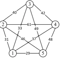
because the reverse routes are ignored. Figure 1 shows a simple TSP with five

nodes.

In this example, one of the best solutions is (2 → 1 → 5 → 4 → 3 → 2) with a cost of 190. Another repeated solution with the same cost but a different starting node is (1 → 5 → 4 → 3 → 2 → 1).

4. The HCA-TSP Approach and Procedure

Typically, the input of the HCA algorithm is represented as a graph. To solve the TSP, the input to the HCA will be a fully connected graph that represents the problem solution space. The graph has a set of nodes (cities) and set of undi-rected edges (roads) between the nodes. The characteristics associated with each edge are the initial amount of soil and edge depth. The HCA uses a set of artifi-cial water drops to generate solutions, where each water drop has three proper-ties: velocity, amount of carried soil, and solution quality. The procedure of HCA is specified in the following steps:

1) Initialization of the variables and read the problem data.

2) Distribution of the water drops on the nodes of the graph at random. 3) Repeat steps 4) to 7) until termination conditions are met.

4) The flow stage (repeat sub-steps a) - d) until temperature reaches a specific value).

A water drop iteratively constructs a solution for the problem by continuously moving between the nodes.

a) Choosing next node

The movements are affected by the amount of soil and the path depths. The

probability of choosing node j from node i is calculated using Equation (6).

( )

(

( )

)

(

( )

)

( )

(

( )

)

(

( )

)

2 2

, ,

WD i

k vc WD

f Soil i j g Depth i j

P j

f Soil i k g Depth i k

∉

× =

×

∑

(6)

where WD

( )

i

[image:8.595.326.424.613.707.2]

P j is the probability of choosing node j from node i, and vc is the

Figure 1. TSP instance with five nodes.

3

2 4

1 5

31 40

46 61 33 49

42

48

(9)

visited list of each water drop. The f(Soil(i, j))is equal to the inverse of the soil

between i and j, and is calculated using Equation (7).

( )

(

,

)

1

_{( )}

,

f Soil i j

Soil i j ε

=

+ (7)

ε = 0.01 is a small value that is used to prevent division by zero. The second

factor of the transition rule is the inverse of depth, which is calculated based on Equation (8).

( )

(

,

)

1

_{( )}

,

g Depth i j

Depth i j

= ₍₈₎

Depth (i, j) is the depth between two nodes i and j, and calculated by dividing

the length of the path by the amount of soil. The depth of the path needs to be updated when the amount of soil existing on the path changes. The depth is up-dated as follows:

( )

,

_{( )}

( )

, ,

Length i j Depth i j

Soil i j

= ₍₉₎

After selecting the next node, the water drop moves to the selected node and marks it as visited.

b) Update velocity

The velocity of a water drop might be increased or decreased while it is

mov-ing. Mathematically, the velocity of a water drop at time (t + 1) is calculated

us-ing Equation (10).

( )

2 2

( )

1 _, 100 _,

WD WD WD

WD WD t t t

t t WD WD

V V V

V K V

Soil i j Soil Depth i j

α

ψ +

   

 

= × + _ _+ +_ _+ (10)

where VtWD+1 is the current water drop velocity, and K is a uniformly distributed

random number between [0, 1] that refers to the roughness coefficient. Alpha

(α) is a relative influence coefficient that emphasizes this term in the velocity

update equation and helps the water drops to emphasize and favor the path with fewer soils over the other factors. The expression is designed to prevent one wa-ter drop from dominating the other drops. That is, a high-velocity wawa-ter drop is able to remove more soil than slower ones. Consequently, the water drops are more likely to follow the carved paths, which may guide the swarm towards local optimal solution.

c) Update soil

Next, the amount of soil existing on the path and the depth of that path are updated. A water drop can remove (or add) soil from (or to) a path while mov-ing based on its velocity. This is expressed by Equation (11).

( )

_{( )}

(

)

(

)

( )

_{( )}

(

)

2

1

, , if Erosion

, ,

1

, , else Deposition

,

WD WDS

V

PN Soil i j Soil i j V Avg all

Depth i j Soil i j

PN Soil i j Soil i j

Depth i j

∆ 

∗ − − ≥

 

 

 = 

_ _∗ _₊ ₊

 

 ∆



(10)

PN represents a coefficient (i.e., sediment transport rate, or gradation

coeffi-cient) that may affect the reduction in the amount of soil. The increasing soil amount on some paths favors the exploration of other paths during the search process and avoids entrapment in local optimal solutions. The rate of change in

the amount of soil existing between node i and node j depends on the time

needed to cross that path, which is calculated using Equation (12).

( )

,

1

, _WD

i j Soil i j

time

∆ = ₍₁₂₎

such that,

( )

,

1

,

WD

i j WD

t Distance i j time

V+

= ₍₁₃₎

In HCA, the amount of soil the water drop carries reflects its solution quality. Therefore, the water drop with a better solution will carry more soil, which can be expressed by Equation (14).

( )

,

WD WD

WD Soil i j

Soil =Soil +∆ _ψ ₍₁₄₎

One iteration is considered complete when all water drops have generated

so-lutions based on the problem constraints (i.e., when each water drop has visited

each node). A solution represents the order of visiting all the nodes and return-ing to the startreturn-ing node. The qualities of the evaluated solutions are used to up-date the temperature.

d) Update temperature

The new temperature value depends on the solution quality generated by the water drops in the previous iterations. The temperature will be increased as fol-lows:

(

1

)

( )

Temp t+ =Temp t + ∆Temp₍₁₅₎

where,

( )

0

otherwise 10

Temp t D D

Temp

Temp t

β ∆

∆ ∆

  

∗ >

  

 _ _

=   

(16)

and where coefficient β is determined based on the problem. The difference

(∆D) is calculated using Equation (17).

D MaxValue MinValue−

∆ = (17)

Such that,

(

)

(

)

max Solutions Quality min Solutions Quality

MaxValue WDs

MinValue WDs

= _ _

= _ _ (18)

According to Equation (17), increase in temperature will be affected by the

difference between the best solution (MinValue) and the worst solution (

(11)

high enough to evaporate the water drops. Thus, the flow stage may run several times before the evaporation stage starts. When the temperature increases and reaches a specified value, the evaporation stage is invoked.

5) The evaporation stage:

A certain number of water drops evaporates based on the evaporation rate. The evaporation rate is determined by generating a random number between one and the total number of water drops (see Equation 19).

(

)

Evaporation rate Random_Integer 1,= N (19)

The evaporated water drops are selected by the roulette wheel technique. The evaporation process is an approach to avoid stagnation or local-optimal solu-tions.

6) The condensation stage:

The condensation stage is executed as a result of the evaporation process, which is a problem-dependent process and can be customized to improve the

solution quality by performing certain tasks (i.e., local improvement method).

The condensation stage collides and merges the evaporated water drops,

elimi-nating the weak drops and favoring the best drop (i.e., the collector), see

Equa-tion (20).

(

)

₍

(

1 2

₎

)

1 2

Bounce , , Similarity 50%

,

Merge , , Similarity 50%

WD WD OP WD WD

WD WD

< 

=  _≥

 (20)

Finding the similarity between the solutions is problem-dependent, and measures how much two solutions are close to each other. For the TSP, the si-milarities between the solutions of the water drops are measured by the

Ham-ming distance [32]. When two water drops collide and merge, one water drop

will (i.e., the collector) become more powerful by eliminating the other one and

acquires its characteristics (i.e., its velocity). The merging operation is useful to

eliminate one of the water drops as they have similar solutions. On the other hand, when two water drops collide and bounce off, they will directly share in-formation with each other about the goodness of each node, and how much a node contributes to their solutions. The bounce-off operation generates infor-mation that is used later to refine the water drops’ solution quality in the next cycle by emphasis on the best nodes. The information is available and accessible to all water drops and helps them to choose a node that has a better contribution from all the possible nodes at the flow stage. For the TSP, the evaporated water drops share their information regarding the most promising nodes sequence. Within this exchange, the water drops will favor those nodes in the next cycle. Finally, the condensation stage is used to update the global-best solution found up to that point. With regard to temperature, determining the appropriate tem-perature values is through trial and error, and appropriate values for this

prob-lem were identified through experimentation. The values (Table 1) have been

(12)

[image:12.595.210.535.89.249.2]

Table 1. HCA parameters and their values.

Parameter name Parameter value

Number of water drops Equal to number of nodes Maximum number of iterations Triple the number of nodes

Initial soil on each edge 10,000

Initial velocity 100

Initial depth Edge length/soil on that edge

Initial carrying soil 1

Velocity updating α = 2

Soil updating PN = 0.99

Initial temperature 50, β = 10

Maximum temperature 100

7) The precipitation stage:

This precipitation is considered as a termination stage, as the algorithm has to check whether the termination condition is met. If the condition has been met, the algorithm stops with the last global-best solution. Otherwise, this stage is re-sponsible for reinitializing all the dynamic variables, such as the amount of the soil on each edge, depth of paths, the velocity of each water drop, and the amount of soil it holds. The re-initialization of the parameters happens after certain iterations and helps the algorithm to avoid being trapped in local optima, which may affect the algorithm’s performance in the next cycle. Moreover, this stage is considered as a reinforcement stage, which is used to place emphasis on the collector drop. This is achieved by reducing the amount of soil on the edges that belong to the best water drop solution, see Equation (21).

( )

, 0.9

( ) ( )

, , , WD

Soil i j = ∗soil i j ∀ i j ∈Best ₍₂₁₎

The idea behind that is to favor these edges over the other edges in the next cycle. These stages are repeated until the maximum number of iterations is reached. The HCA goes through a number of cycles and iterations to find a

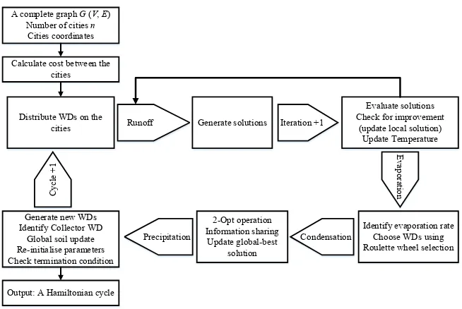
solu-tion to a problem. Figure 2 explains the steps in solving the TSP by HCA.

4.1 .

Solution Representation

In this paper, the TSP is assumed to be symmetric, and acting on a fully con-nected graph. The candidate TSP solutions are stored in a matrix, where each row represents a different solution generated by a water drop. Therefore, a water drop solution consists of the order of the visited nodes (with no repeat visits).

The length of each row (i.e. the number of columns) is denoted by n and

deter-mined by the total number of nodes (see Equation 22).

1 2 3

1 2 1 2

Solutions 1 2

1 2

n

WD n

 

 

=

 

 

       



(13)

[image:13.595.210.537.67.286.2]

Figure 2. TSP solution procedure of HCA.

4.2. Local Improvement Operation

The quality of generated tours can be improved by many operations, such as

k-Opt (where k = 2, 3, or 4) [33] [34]. These operations enhance the

perfor-mance of the algorithm and minimize the number of iterations to reach the op-timal solution. In the present problem, we apply the 2-Opt operation on the se-lected water drops that will evaporate at the condensation stage. The 2-Opt op-eration swaps the order of two edges at one part of the tour and keeps the tour connected. The swapping results in a new tour, which is accepted if it minimizes

the total cost [35]. This operation is repeated until a stopping criterion is met,

such as no further improvements after a certain number of exchanges, or when

the maximum number of exchanges is reached. Figure 3 demonstrates the

oper-ation of 2-Opt. In this example, the algorithm selects edges (2, 7) and (3, 8), and consecutively creates new edges (2, 3) and (7, 8). The order of the nodes between the two edges must also be reversed.

5. Experimental Results and Analysis

The HCA was tested and evaluated on two groups of TSP instances; structural and benchmark. The runtime and solution quality of the benchmark results were compared with those of other algorithms.

The HCA parameter values used for TSP are listed in Table 1. The parameters

values are set after conducting some preliminary experiments.

The depth values had a very small value. Therefore, it has been normalized to be within [1 - 100]. The amount of soil has been restricted to be within a maxi-mum and minimaxi-mum value for avoiding negative values. The maximaxi-mum value is regarded as the initial value, while the minimum value is fixed to equal one. The algorithm was implemented using MATLAB. All the experiments were con-ducted on a computer with Intel Core i5-4570 (3.20 GHz) CPU and 16 GB RAM,

Distribute WDs on the

cities Generate solutions

Evaluate solutions Check for improvement

(update local solution) Update Temperature

Identify evaporation rate Choose WDs using Roulette wheel selection 2-Opt operation

Information sharing Update global-best

solution Generate new WDs

Identify Collector WD Global soil update Re-initialise parameters Check termination condition

Runoff Iteration +1

Ev

ap

ora

tio

n

C

yc

le

+

1

Precipitation Condensation A complete graph G (V, E)

Number of cities n

Cities coordinates Calculate cost between the

cities

(14)

Figure 3. Example of removing an intersection by 2-Opt.

under Microsoft Windows 7 Enterprise as an operating system.

5.1. Structural TSP Instances

To assess the validity of the generated output, we designed and generated syn-thetic TSP structures with different geometric shapes (circle, square, and trian-gle). These TSP structures are easier to evaluate than randomized instances. Several instances with different numbers of nodes were generated for each structure, and were input to the HCA algorithm with and without the 2-Opt

op-eration. The percentage difference (i.e., the deviation percentage) between the

obtained and the optimal value was calculated as follows:

(

Obtained Value Optimal Value

)

Difference 100%

Optimal Value −

= × ₍₂₃₎

In the circular structure, the circle circumference was divided into various numbers of nodes. Note that the number of nodes influences the inter-nodal distance, with fewer nodes increasing the distance between nodes. The node number was varied as 25, 50, 75, 100, 125, and 150. By dividing the circumfe-rence of the circle into a specific number of nodes, the first and last nodes will have the same coordinate. The shortest path length was calculated by the circle

circumference formula (2 × π × r). The circle was centered at (1, 1) and its

di-ameter was set to 2 (i.e., r = 1). Consequently, its circumference was 6.28. The

obtained results are reported in Table 2.

As shown in Table 2, the HCA found the shortest path in each instance of this

structure, both with and without the 2-Opt operation. The circle instances are relatively easy to solve because the distance decreases with increasing number of nodes. Thus, the soil amount will be reduced more quickly on shorter edges than

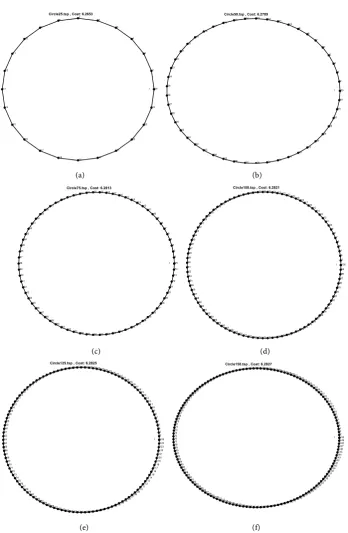
on longer edges, steering the algorithm towards the shorter edges. Figure 4

shows the output of the HCA on circular TSPs with different numbers of nodes. Next, the TSP was solved on a square structure. Here, the nodes were evenly

spaced in an N × N grid. The shortest tour distance was the product of the

number of nodes and the distance between the nodes (assumed as one unit). For example, in the 16-point (8 × 8) grid, the shortest path was (1 × 16 = 16). For an odd number of nodes, the cost of traveling to the last node was based on the length of the hypotenuse (1.41 in the present examples). Ten instances with dif-ferent numbers of nodes were generated, and solved by the HCA with and

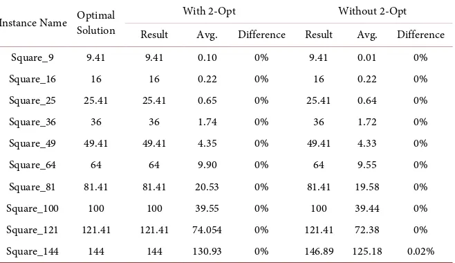
without the 2-Opt operation. The results are listed in Table 3.

As shown in Table 3, the HCA obtained the optimal results (the shortest

path) both with and without the 2-Opt operation. The exception was “Square_144”, whose solution deviated very slightly from the optimal. The

1 8

2 3

7 4

6

5 1

8

2 3

7 4

(15)

DOI: 10.4236/ajor.2018.83010 147 American Journal of Operations Research (a) (b)

(c) (d)

[image:15.595.189.538.60.594.2]

(e) (f)

Figure 4. TSP solutions on circular grids. (a) Circle_25, Cost = 6.28; (b) Circle_50, Cost = 6.28; (c) Circle_75, Cost = 6.28; (d) Circle_100, Cost = 6.28; (e) Circle_125, Cost = 6.28; (f) Circle_150, Cost = 6.28.

outputs of HCA with 2-Opt on square grids of different sizes are shown in

Fig-ure 5.

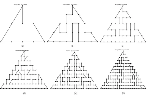
Finally, the TSP was solved on an equilateral triangular grid. The number of

nodes was varied as 9, 25, 49, 81, 121, and 169. Table 4 lists the obtained results

with and without the 2-Opt operation.

0 0 2 0 4 0 6 0 8 1 1 2 1 4 1 6 1 8 2

0 0.2 0.4 0.6 0.8 1 1.2 1.4 1.6 1.8

2 Circle25.tsp , Cost: 6.2653

3

2

1 25

24 23 22 21 20 19 18 17 16 15 14 13 12 11 10 9

8 7 6 5 4 0 0.2 0.4 0.6 0.8 1 1.2 1.4 1.6 1.8

2 Circle50.tsp , Cost: 6.2789

18 19 20 21 22 23 24 25 26 27 28 29 30 31 32 33 34 35

36 37 38 39 40 41 42 43 44 45 46 47 48 49 50 1 2 3 4 5 6 7 8 9 10 11 12 13 14 15 16 17

0 0.2 0.4 0.6 0.8 1 1.2 1.4 1.6 1.8 2

0 2 4 6 8 1 2 4 6 8

2 Circle75.tsp , Cost: 6.2813

27 28 29 30 31 32 33 34 35 36 37 38 39 40 41 42 43 44 45 46 47 48 49 50 51₅₂

53 54_{55 56 57 58 59} 60 61 62 63

64 65 66 67 68 69 70 71 72 73 74 75 1 2 3 4 5 6 7 8 9 10 11 12 13 14 15 16 17 18 19 20 21 22 23 24 25 26 0 0.2 0.4 0.6 0.8 1 1.2 1.4 1.6 1.8

2 Circle100.tsp , Cost: 6.2821

65 64 63 62 61 60 59 58 57 56 55 54 53 52 51 50 49 48 47 46 45 44 43 42 41 40 39

38 37 36 35

34 33

32 31 30 29 28 27 26 25 24 23 22 21 20₁₉ 18 17 16 15 14 13 12 11 10 9 8 7 6 5 4 3 2 1 100

99 98 97 96 95 94 93 92 91 90 89 88 87 86 85 84 83 82 81 80 79 78 77 76 75 74 73 72 71 70 69 68 67 66

0 0.2 0.4 0.6 0.8 1 1.2 1.4 1.6 1.8 2

0 .2 .4 .6 .8 1 .2 .4 .6 .8

2 Circle125.tsp , Cost: 6.2825

86 87

88 89 90 91 92 93 94 95 96 97 98 99 100 101 102 103 104

105 106 107 108

109 110 111 112

113 114 115 116

117 118 119 120

121 122 123 124 125 1 2 3 4 5 6 7 8 9 10 11 12 13 14 15 16 17 18 19 20 21 22 23 24 25 26 27 28 29 30 31 32 33 34 35 36 37 38 39 40 41 42 43 44 45 46 47 48 49 50 51 52 53 54 55 56 57 58 59 60 61 62 63 64 65 66 67 68 69 70 71 72 73 74 75 76 77 78 79₈₀

81₈₂ 83₈₄

85

0 0.2 0.4 0.6 0.8 1 1.2 1.4 1.6 1.8 2

X-axis 0 0.2 0.4 0.6 0.8 1 1.2 1.4 1.6 1.8

2 Circle150.tsp , Cost: 6.2827

150 1 2

3 4 5 6 7 8 9 10 11 12 13 14 15 16 17 18 19 20 21 22 23 24 25 26 27 28 29 30 31 32 33 34 35 36 37 38 39 40 41 42 43 44 45 46 47 48 49 50 51 52 53 54 55 56 57 58 59 60 61 62 63 64 65 66 67 68 69 70 71 72 73 74 75 76 77 78 79 80 81 82 83 84 85 86₈₇

88 89

90₉₁ 92₉₃

94₉₅ 96₉₇

98_{99 100} 101_{102 103}

104 105 106_{107 108 109 110 111 112 113 114 115 116 117 118 119} 120 121 122 123 124 125 126

127 128 129 130 131

132 133 134 135

136 137 138 139

140 141 142 143

(16)

[image:16.595.211.541.90.226.2]

Table 2. TSP results on a circular structure.

Instance

Name Solution Optimal

[image:16.595.209.542.257.458.2]

With 2-Opt Without 2-Opt Result Avg. Difference Result Avg. Difference Circle_25 6.28 6.28 0.72 0% 6.28 0.65 0% Circle_50 6.28 6.28 4.48 0% 6.28 4.47 0% Circle_75 6.28 6.28 15.43 0% 6.28 15.13 0% Circle_100 6.28 6.28 38.60 0% 6.28 37.23 0% Circle_125 6.28 6.28 80.49 0% 6.28 74.50 0% Circle_150 6.28 6.28 146.68 0% 6.28 136.99 0%

Table 3. TSP results on a square structure.

Instance Name Optimal _Solution With 2-Opt Without 2-Opt Result Avg. Difference Result Avg. Difference Square_9 9.41 9.41 0.10 0% 9.41 0.01 0%

Square_16 16 16 0.22 0% 16 0.22 0%

Square_25 25.41 25.41 0.65 0% 25.41 0.64 0%

Square_36 36 36 1.74 0% 36 1.72 0%

Square_49 49.41 49.41 4.35 0% 49.41 4.33 0%

Square_64 64 64 9.90 0% 64 9.55 0%

Square_81 81.41 81.41 20.53 0% 81.41 19.58 0% Square_100 100 100 39.55 0% 100 39.44 0% Square_121 121.41 121.41 74.054 0% 121.41 72.38 0% Square_144 144 144 130.93 0% 146.89 125.18 0.02%

Table 4. TSP results on a triangular structure.

Instance Name Optimal _Solution With 2-Opt Without 2-Opt Result Avg. Difference Result Avg. Difference Square_9 9.41 9.41 0.10 0% 9.41 0.01 0%

Square_16 16 16 0.22 0% 16 0.22 0%

Square_25 25.41 25.41 0.65 0% 25.41 0.64 0%

Square_36 36 36 1.74 0% 36 1.72 0%

Square_49 49.41 49.41 4.35 0% 49.41 4.33 0%

Square_64 64 64 9.90 0% 64 9.55 0%

Square_81 81.41 81.41 20.53 0% 81.41 19.58 0% Square_100 100 100 39.55 0% 100 39.44 0% Square_121 121.41 121.41 74.054 0% 121.41 72.38 0% Square_144 144 144 130.93 0% 146.89 125.18 0.02%

[image:16.595.211.540.488.678.2]

(17)

DOI: 10.4236/ajor.2018.83010 149 American Journal of Operations Research (a) (b)

(c) (d)

(e) (f)

(g) (h)

0 0.2 0.4 0.6 0.8 1 1.2 1.4 1.6 1.8 2

0 0.2 0.4 0.6 0.8 1 1.2 1.4 1.6 1.8 2 Y-axis

Square9.tsp , Cost: 9.4142

1 4 7

8 9 6

3

2 5

0 0.5 1 1.5 2 2.5 3

0 0.5 1 1.5 2 2.5

3 4 Square16.tsp , Cost: 16 8

7 11

12 16

15 14 13 9 10 6 5 1 2 3

0 0.5 1 1.5 2 2.5 3 3.5 4

0 0.5 1 1.5 2 2.5 3 3.5

4 5 10 Square25.tsp , Cost: 25.4142

4

3

2

1 6

7

8 13

14 19

18

17 12

11 16 21

22 23 24 25 20 15 9

0 0 5 1 1 5 2 2 5 3 3 5 4 4 5 5

0 0.5 1 1.5 2 2.5 3 3.5 4 4.5 5 Y-axis

Square36.tsp , Cost: 36

14 15 9 8 7 1 2 3 4 5

6 12

11

10 16

17

18 24 30 36

35 34 33 27 28 29 23 22 21

20 26 32

31 25 19 13

0 1 2 3 4 5 6

0 1 2 3 4 5 6 Y-axis

13 14 7 6 5 4

3 10

11

12 19

18

17 24

23 16 9 2

1 8 15 22 29 36 43

44 45 38 37 30 31 32 25

26 33

34 41

40

39 46

47 48 49 42 35 28 27 20 21

0 1 2 3 4 5 6 7

0 1 2 3 4 5 6 7 Y-axis

44 52

53 54 55 47 39

40 48 56 64

63 62 61 60 59 58 57 49 41 33

34 42 50

51 43 35 27 26 25 17 9 1 2

3 11

10 18

19 20 12 4

5 13 21

22 14 6 7

8 16

15 23

24 32

31

30 38 46

45 37 29

28 36

0 1 2 3 4 5 6 7 8

0 1 2 3 4 5 6 7 8 Y-axis

35 44

43

42 51

52 61

60 69

70 71 62 53

54 63 72 81

80 79 78 77 76 67 68 59 58

57 66 75

74 73 64 65 56 55 46 37 28 19 20 11 10 1 2 3 4 5 6

7 16

15

14

13

12 21 30

29 38 47

48 39

40 49

50 41 32 31 22 23

24 33

34 25 26 17 8

9 18 27 36 45

0 1 2 3 4 5 6 7 8 9

0 1 2 3 4 5 6 7 8

9 Square100.tsp , Cost: 100

28 18 19 20 10 9 8

7 17

16 6

5 15 25

24 14 4

3 13 23

22 12 2

1 11 21 31

32 42

41 51 61 71

72 82

81 91

92 93 94 95 96 97 98 99 100 90 80

79 89

88 78 68 69 70 60 50

49 59

58 48

47

46 56

57 67

66

65

64 74

75 76

77 87

86 85 84 83 73 63 62 52 53 54 55 45 44 43 33 34 35 36 26

27 37

38 39 40 30

(18)

[image:18.595.136.538.68.254.2]

DOI: 10.4236/ajor.2018.83010 150 American Journal of Operations Research (i) (j)

Figure 5. TSP solutions on square grids. (a) Cost = 9.41; (b) Cost = 16; (c) Cost = 25.41; (d) Cost = 36; (e) Cost = 49.41; (f) Cost = 64; (g) Cost = 81.41; (h) Cost = 100; (i) Cost = 121.41; (j) Cost = 144.

results. The TSP is more difficult on the triangular structure than on the other structures, because many hypotenuses connect the nodes to different layers. The outputs of the HCA using 2-Opt on triangular grids with different node

num-bers are reported in Figure 6.

The average execution times for solving all the TSP structural instances by

HCA are presented by Figure 7. The execution time of the HCA increases with

increasing number of nodes because of the information sharing process. With increasing number of nodes the solution space increases exponentially, a defin-ing characteristic of NP-hard problems which also affects execution time. The execution time also largely depends on the implementation of the algorithm, and on the compilers, machines specifications, and operating systems used.

Figure 7 shows that the 2-Opt operation has little effect on the execution time in small instances (problems with a low node count), but noticeably increases the execution time in larger problems. However, 2-Opt was found to improve the quality of the solution for structures with a high number of nodes.

5.2. Benchmark TSP Instances

Next, the HCA was applied to a number of standard benchmark instances from

the TSPLIB library [36]. The selected instances have different structures with

different numbers of cities. Some of these instances are geographical and based on real city maps; others are based on VLSI applications, drilling, and printed circuit boards. The edge-weights (distances) between the nodes were calculated by the Euclidean distance (Equation (1)), and rounded to integers. The TSP file

format is detailed in Reinelt [37]. On the benchmark problems, the HCA was

combined with the 2-Opt operation, which was found to improve the solution quality in structural instances with large numbers of nodes. The results are

pre-sented in Table 5. In this table, the number in each instance name denotes the

number of cities, and the difference column denotes the percentage difference

0 1 2 3 4 5 6 7 8 9 10

Y

axis

Square121.tsp , Cost: 121.4142

23 34 45 46 47 48 59

58 69

70 81 92

91 80

79 68 57

56 67 78 89 90 101

100 111 112 113 102 103 114

115 104 93

94 105 116 117 118 119 120 121 110

109

108 97 86 87 98

99 88 77 66 55 44 33 22 11

10 21 32 43 54 65 76

75 64 53

52 63 74 85 96 107

106 95 84

83

82 71 60 61 72

73 62 51 40 41 42 31

30 19 20 9

8

7

6

5 16

15 4

3

2

1 12 13 14 25

26 27 17 18 29

28 39 50

49 38

37

36

35 24

0 2 4 6 8 10

0 2 4 6 8 10 12

Y-axis

10 9 8 7 6 18 30

29 28 27 26 14 15 16 17 5 4 3 2

1 13 25 37 49 61 62 50 38 39 51

52 40 41 42 43 55

56 44 32 31 19 20 21 33 45

46 34 22

23 35 47 59 58

57 69 81 93 105 104 92 80 68 67 66 54 53 65

64

63 75 87 99 98 86 74

73 85 97 109 121 133 134 135 136 137 125 124 123 122 110 111 112 100 88 76 77 78 79 91 103

102 90 89 101 113

114 126 138 139 127 115 116 117 129

128 140 141 142 143 144 132 131 130 118 119 120 108 96 84 83 95 107

(19)

DOI: 10.4236/ajor.2018.83010 151 American Journal of Operations Research (a) (b) (c)

[image:19.595.64.538.59.367.2]

(d) (e) (f)

[image:19.595.210.537.410.572.2]

Figure 6. TSP solutions on equilateral triangular grids. (a) Cost = 10.24; (b) Cost = 27.07; (c) Cost = 51.899; (d) Cost = 84.727; (e) Cost = 125.556; (f) Cost = 174.38.

Figure 7. Relationship between HCA execution time and instance size of TSP on circular, square and triangular grids.

from the optimal solution using Equation (7).

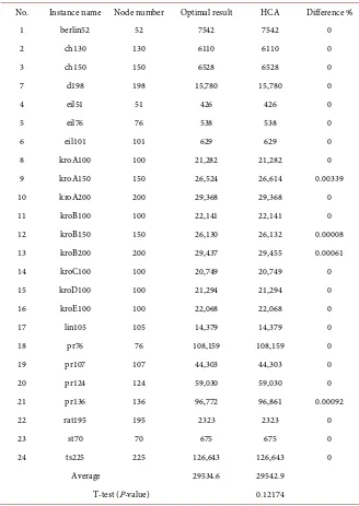
Table 5 shows that the HCA achieved a high performance when solving TSP. The HCA found the optimal solution in 20 out of 24 instances, and the

differ-ences in the other instances were minor. According to the P-value, there is no

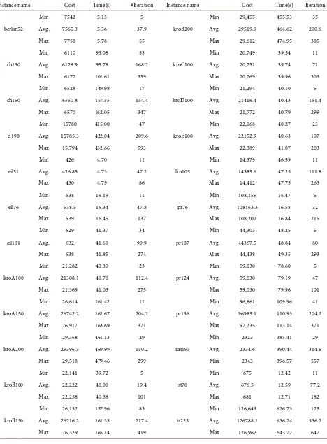
significant difference between the results. Table 6 reports the minimum,

aver-age, and maximum values of the cost, time and iteration number among 10 HCA executions for each instance.

0 0 5 1 1 5 2 2 5 3 3 5 4

0 0.2 0.4 0.6 0.8 1 1.2 1.4 1.6 1.8

2 Triangle9.tsp , Cost: 10.2426

4 5

8 7

9

6

1 2 3

0 1 2 3 4 5 6 7 8

0 0.5 1 .5 2 2.5 3 3.5

17

11 12

18

22 23

25

24

21

15 16

9 8 7 6 14 20 19 13 5 4 3 2 1 10

0 2 4 6 8 10 12

0 1 2 3 4 5 6 Y-axis

Triangle49.tsp , Cost: 51.8995

45 44 43

37 38

30 29 28

18 19 20 21

31

39 40

32 33

24 13 12 11 23 22 10 9 8 7 6 5 4 3 2 1

14 15 16 17

27 26 25

34 35 36

42 41

46 49

47 48

0 2 4 6 8 10 12 14 16

0 1 2 3 4 5 6 7 8 Y-axis

Triangle81.tsp , Cost: 84.7279

74 73 67 66 58 57 47 46 34 33 19 18

1 2 3 4 5 6 7 8 9 10 11 12 13 14 15 16 17 32 31 45 56 44 30 29 43 42 28 27 26 25 24 23 22 21 20

35 36 37

49 48

59

50

38 39

51 61 60

68 69 70

62 63

52

40 41

53 54 55

65 64 72 71 77 76 80 75 79 81 78

0 2 4 6 8 10 12 14 16 18 20

0 1 2 3 4 5 6 7 8 9

81 80

66 67

51 50 49 48 47 63 62 46

28 29 30 31

11 10 9 8 7 6 5 4 3 2 1

22 23 24

42 41 58 73 59 43

25 26 27

45 44

60 61

75 74

86 87

97 98

106 107

113 114

108 100 90 89 99 88

76 77 78

64 65

79 91 101 109 115 119 118 121 120 117 116 110 102

92 93 94

103

111 112

104 105

95 96

84 85

71 72

57

39 40

21 20 19 18 17 16

36 37 38

56 55 54 53 35 15 14 13 12

32 33 34

52

68 69 70

83 82

0 5 10 15 20

0 2 4 6 8 10

163

157 158

150 151

141 140 128 114 113 97 79 78

58 59 60

80

98 99

81

61 62

82 83

63 64 65

43 42 41 40 39 38 37 36 35

11 12 13 14 15 16 17 18 19 20 21 22

46

23 24 25

48 47 69 68 88 87 67 45 44 66 86 105 104 120 119 133 132 144 143 131

117 118

103 85 84 102 101 100 116 115 129 130

142 153 152 160 159 165 164 168 167 169 166 161

154 155

147 138 137 136 146 145 135 134 121

106 107 108

122 123 124 125

111 110 109 93 92 91 73 72 90 89 71 70 50 49 27 26

1 2 3 4 5 6 7 31 30 29 28

51 52 53 54

74 75

55

33 32

8 9 10

34

56 57

77 76

94 95 96

112 126 127

139 149 148 156 162 0 50 100 150 200 250

0 50 100 150 200

A ver ag e t im e (S ec)

Number of nodes Exection time for HCA

(20)

[image:20.595.209.537.87.550.2]

Table 5. HCA results on benchmark TSP instances.

No. Instance name Node number Optimal result HCA Difference %

1 berlin52 52 7542 7542 0

2 ch130 130 6110 6110 0

3 ch150 150 6528 6528 0

7 d198 198 15,780 15,780 0

4 eil51 51 426 426 0

5 eil76 76 538 538 0

6 eil101 101 629 629 0

8 kroA100 100 21,282 21,282 0

9 kroA150 150 26,524 26,614 0.00339

10 kroA200 200 29,368 29,368 0

11 kroB100 100 22,141 22,141 0

12 kroB150 150 26,130 26,132 0.00008

13 kroB200 200 29,437 29,455 0.00061

14 kroC100 100 20,749 20,749 0

15 kroD100 100 21,294 21,294 0

16 kroE100 100 22,068 22,068 0

17 lin105 105 14,379 14,379 0

18 pr76 76 108,159 108,159 0

19 pr107 107 44,303 44,303 0

20 pr124 124 59,030 59,030 0

21 pr136 136 96,772 96,861 0.00092

22 rat195 195 2323 2323 0

23 st70 70 675 675 0

24 ts225 225 126,643 126,643 0

Average 29534.6 29542.9

T-test (P-value) 0.12174

The results in Table 6 demonstrate the efficiency and effectiveness of the

HCA algorithm. In particular, the average result and optimal solution are very close in all instances. The maximum difference was 0.00823% on the kroA150 benchmark, and zero on the pr124 benchmark. Moreover, the HCA optimized the solution on most benchmarks within a few iterations. This early convergence is attributed to information sharing among the water drops, and the use of the 2-Opt operation in the condensation stage. The solutions to the benchmark

in-stances are displayed in the Figure S1 (Appendix).

(21)

[image:21.595.67.535.91.726.2]

Table 6. Minimum, average, and maximum HCA results on benchmark TSP instances.

Instance name Cost Time(s) #Iteration Instance name Cost Time(s) Iteration

berlin52

Min 7542 5.15 5

kroB200

Min 29,455 455.53 35

Avg. 7565.3 5.36 37.9 Avg. 29519.9 464.62 200.6

Max 7758 5.78 55 Max 29,612 474.95 305

ch130

Min 6110 93.08 53

kroC100

Min 20,749 39.54 11

Avg. 6128.9 95.79 168.2 Avg. 20,751 39.74 71

Max 6177 101.61 359 Max 20,769 39.96 303

ch150

Min 6528 149.98 17

kroD100

Min 21,294 40.10 5

Avg. 6550.8 157.55 154.4 Avg. 21416.4 40.43 151.4

Max 6570 162.05 347 Max 21,772 40.79 299

d198

Min 15780 415.00 47

kroE100

Min 22,068 40.27 23

Avg. 15785.3 422.04 209.6 Avg. 22152.9 40.63 107

Max 15,794 432.66 593 Max 22,389 41.07 203

eil51

Min 426 4.70 11

lin105

Min 14,379 46.59 11

Avg. 426.85 4.73 47.2 Avg. 14385.6 47.25 111.8

Max 430 4.79 86 Max 14,412 47.75 263

eil76

Min 538 16.19 11

pr76

Min 108,159 16.47 5

Avg. 538.5 16.34 47.8 Avg. 108163.3 16.58 32

Max 539 16.45 137 Max 108,202 16.84 215

eil101

Min 629 41.37 34

pr107

Min 44,303 48.25 5

Avg. 632 41.60 99.9 Avg. 44367.5 48.84 80

Max 638 41.85 274 Max 44,438 49.35 293

kroA100

Min 21,282 40.39 23

pr124

Min 59,030 78.60 5

Avg. 21308.1 40.70 112.4 Avg. 59,030 79.19 47

Max 21,369 41.03 275 Max 59,030 79.96 101

kroA150

Min 26,614 161.42 11

pr136

Min 96,861 109.96 41

Avg. 26742.2 162.67 204.2 Avg. 96985.1 110.93 204.2

Max 26,917 163.69 371 Max 97,235 113.14 371

kroA200

Min 29,368 461.13 29

rat195

Min 2323 385.41 29

Avg. 29396.3 469.99 150.2 Avg. 2334.6 390.44 314.6

Max 29,518 479.46 299 Max 2343 396.57 557

kroB100

Min 22,141 39.72 5

st70

Min 675 12.42 11

Avg. 22,222 40.00 19.4 Avg. 676.5 12.59 77.2

Max 22,258 40.38 101 Max 681 12.71 182

kroB150

Min 26,132 157.96 83

ts225

Min 126,643 626.73 125

Avg. 26216.2 161.33 217.4 Avg. 126788.1 636.24 336.2

(22)

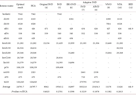
algorithm (WFA), and river formation dynamics (RFD). The comparisons are

summarized in Table 7. The results of the original and a modified IWD

(col-umns 4 and 5, respectively) were taken from [1] and from [38], respectively. The

results of another modified IWD, called the exponential ranking selection IWD

(ERS-IWD; column 6), were extracted from [3]. The results of columns 7 and 8

were taken from [5], who implemented the IWD and their proposed adaptive

IWD on TSP instances. The WWO results (column 9) were taken from [7]. The

WFA and RFD results (columns 10 and 11) were borrowed from [8] and from

[9], respectively. The best results are marked in bold font.

The numbers of instances solved by these algorithms are insufficient for

cal-culating an accurate P-value statistic. Moreover, some of these algorithms

per-form as well as HCA in certain instances. However, as confirmed in Table 7,

[image:22.595.62.538.388.725.2]

HCA outperforms the original IWD algorithm and its various modifications. One plausible reason for the poor performance of the IWD algorithm is the premature convergence and stagnation in local optimal solutions. In contrast, HCA can escape from local optima by exploiting the depths of the paths along with the soil amount. These actions diversify the solutions. The most competi-tive opponent to HCA was WFA, which also optimized the solutions in the tested instances. In contrast, the WWO performed poorly because this algorithm

Table 7. Best results of HCA, the original IWD, modified IWDs, WWO, WFA, and RFD.

Instance name Optimal _result HCA Original IWD ₍₄₎ IWD ₍₅₎ ERS-IWD ₍₆₎

Adaptive IWD

WWO

(9) WFA (10) RFD (11) IWD

(7) AIWD (8)

berlin52 7542 7542 - 7542 - - - -

ch130 6110 6110 - - 6316 - - 6338 6110 -

ch150 6528 6528 - - - 7014 6528 -

eil51 426 426 471 426 429 434 426 427 426 441.9

eil76 538 538 559 540 545 552 538 557 538 -

eil101 629 629 - 639 654 - - - 629 -

kroA100 21,282 21,282 23,156 21,429 21,959 23,183 21,304 21,668 21,282 -

kroA150 26,524 26,614 - - - 26,524 -

kroA200 29,368 29,368 - - 31,680 - - 31,064 29,368 -

kroC100 20,749 20,749 - 20,816 - - - -

lin105 14,379 14,379 - 14,393 14,696 - - - - -

pr76 108,159 108,159 - 109,608 - - - -

rat195 2323 2323 - - - 2461 2338 -

st70 675 675 - 676 - 710 675 - - -

ts225 126,643 126,643 - - - 275791 127325 - - -

(23)

was originally designed for continuous-domain problems, and its operations need adjustment for combinatorial problems. Moreover, the WWO adopts a re-ducing population-size strategy, which degrades its performance in some prob-lems. Finally, the WWO suffers from slow convergence because it depends only on the altitude of the nodes.

The performances of HCA, IWD, adaptive IWD (AIWD) and modified IWD

(MIWD) are further compared in Table 8. The best and average results of IWD

and AIWD were taken from [5], while those of MIWD were taken from [6].

This comparison aims to compare the robustness of HCA and other algo-rithms. Despite there being no significant differences between the results (best, average), the average results are closer to the optimal in HCA than in the other

algorithms, suggesting the superior robustness of HCA. Table 9 compares the

runtimes of the HCA, IWD and AIWD. The best and average execution times

and iteration numbers of the IWD algorithms were taken from [5].

According to Table 9, HCA reaches the best solution after fewer iterations

than IWD and AIWD. This result confirms the superior efficiency of HCA. Moreover, adding the other stages of the water cycle did not affect the average

execution time of HCA. Figure 8 plots the average execution times of the three

algorithms implemented on five benchmark problems.

Optimal-solution searching by HCA was compared with those of other well-known algorithms, namely, an ACO algorithm combined with fast opposite

gradient search (FOGS-ACO) [39], a genetic simulated annealing ant colony

system with PSO (GSAACS-PSO) [40], an improved discrete bat algorithm

(IBA) [27], set-based PSO (S-CLPSO) [41], a modified discrete PSO with a newly

introduced mutation factor C3 (C3D-PSO); results taken from [23], an adaptive

simulated annealing algorithm with greedy search (ASA-GS) [11], the firefly

al-gorithm (FA) [42], a hybrid ACO enhanced with dual NN (ACOMAC-DNN)

[43], a discrete PSO (DPSO) [26], a self-organizing neural network using the

immune system (ABNET-TSP) [44], and an improved discrete cuckoo search

[image:23.595.211.539.552.727.2]

algorithm (IDCS) [45]. Table 10 summarizes the comparison results.

Table 8. Best and average results of HCA, IWD, AIWD, and MIWD.

Instance Name

HCA IWD AIWD MIWD

Best Avg. Best Avg. Best Avg. Best Avg. Eil51 426 426.85 434 443.2 426 428.4 428.98 432.62

St70 675 676.5 710 724.93 675 682.5 677.1 684.08 Eil76 538 538.5 552 564.43 538 542.86 549.96 558.23 KroA100 21282 21308.1 23183 23548.37 21,304 21586.73 21407.57 21904.03

rat195 2323 2334.6 2461 2480.6 2338 2347.8 - - ts225 126643 126788.1 755791 276140.75 127,325 128323.5 - - Average 29912.8 29947.6 130521.8 50650.4 25434.3 25652.0 5765.9 5894.7

(24)

[image:24.595.57.544.89.236.2]

Table 9. Average execution times and best and average iteration numbers in HCA, IWD, and Adaptive IWD.

Instance name HCA IWD Adaptive IWD

Avg. Time (s) Iteration [Best, Avg.] Avg. Time (s) Iteration [Best, Avg.] Avg. Time (s) Iteration [Best, Avg.] eil51 4.73 [57, 47.2] 154.537 [1509, 3000] 180.648 [190, 3000]

st70 12.59 [83, 77.2] 434.193 [960, 3,500] 453.631 [1769, 3500] eil76 16.34 [46, 47.8] 567.208 [2147, 3,500] 571.251 [752, 3500] kroA100 40.7 [89, 112.4] 1364.979 [3698, 3750] 1365.752 [2397, 3750]

rat195 390.44 [401, 314.6] 2023.162 [604, 5000] 2335.9392 [4995, -] ts225 636.24 [365, 336.2] 3969.892 [1, 5000] 4162.92 [3850, 5000]

Average 142.1 1419.0 1511.7

T-test (P-value) for Avg. Time 0.1162 0.1200

Table 10. Best results obtained by HCA and other optimization algorithms.

Instance

name Optimal result HCA

FO

G

S-A

CO

G

SA

A

CS

-PSO IBA

S-C

LPSO

C3

D

-PSO

A

SA

-GS FA

A

CO

M

A

C-DN

N

DPSO

A

BN

ET

-T

SP IDCS

berlin52 7542 7542 7546.6 7542 7542 7542 7544.7 7544.36 - 7542 7542 7542

ch130 6110 6110 - 6141 - - 6110.7 - - - 6145 6110

ch150 6528 6528 - 6528 - - 6530.9 - - - 6602 6528

eil51 426 426 426 427 426 426 426 428.87 428.87 430.01 427 427 426 eil76 538 538 546.83 538 539 538 538 544.37 552.61 546 541 538

eil101 629 629 633.40 630 634 629 640.21 - 638 629

d198 15,780 15,780 - - 15,809 15830.6 15,955.6 - 15,781

kroA100 21,282 21,282 22,414 21,282 21,282 21,282 21,282 21285.4 21285.4 21,408.2 - 21,333 21,282 kroA150 26,524 26,614 - 26,524 - 26,537 26524.9 - - 26,678 26,524 kroA200 29,368 29,368 29,717 29383 - 29,399 29411.5 - - 29,600 29,382 kroB100 22,141 22,141 - 22141 22,140* - 22139.1 22139.1 - - 22,343 22,141 kroB150 26,130 26,132 - 26130 - - 26140.7 - - - 26,264 26,130 kroB200 29,437 29,455 - 29541 - - 29504.2 - - - 29,637 29,448 kroC100 20,749 20,749 - 20,749 20,749 20824.6 20750.8 - - - 20,915 20,749 kroD100 21,294 21,294 - 21,309 21,294 21405.6 21294.3 - - - 21,374 21,294 kroE100 22,068 22,068 - 22,068 22,068 - 22106.3 - - - 22,395 22,068 lin105 14,379 14,379 - 14,379 - 14379 14383 14383 - - 14,379 14,379 pr76 108,159 108,159 108,864 - - 108159 108159 - 108280 - 108,159

pr107 44,303 44,303 - - 44,303 44301.7* 44346 - - - 44,303

pr124 59,030 59,030 - - 59,030 59030.7 59030 - - - 59,030

pr136 96,772 96,861 - - 97,547 96966.3 97182.7 - - - 96,790

rat195 2323 2323 - - - 2345.2 - - - 2324

st70 675 675 678.93 - 675 675 675 677.11 677.11 - 675 - 675

ts225 126,643 126,643 - - - - 126646 - - - - 126,643

Average 29534.6 29542.9 21353.3 16062.2 24479.2 20585.0 5730 29,554 29,669 9587 23,494 16,051 29536.5 P-values versus HCA 0.1120 0.6755 0.3327 0.3088 - 0.1129 0.2684 0.1536 0.3360 0.0014 0.1890

[image:24.595.59.540.268.710.2]