A Robust Incremental Algorithm for Predicting the Motion
of Rigid Body in a Time-Varying Environment
Ashraf Elnagar
Department of Computer Science, University of Sharjah, Sharjah, UAE Email: [email protected]
Received January 30, 2012; revised April 8, 2012; accepted May 5,2012
ABSTRACT
A configuration point consists of the position and orientation of a rigid body which are fully described by the position of the frame’s origin and the orientation of its axes, relative to the reference frame. We describe an algorithm to robus-tly predict futuristic configurations of a moving target in a time-varying environment. We use the Kalman filter for tracking and motion prediction purposes because it is a very effective and useful estimator. It implements a predic-tor-corrector type estimator that is optimal in the sense that it minimizes the estimated error covariance. The target mo-tion is unconstrained. The proposed algorithm may be viewed as a seed for a range of applicamo-tions, one of which is ro-bot motion planning in a time-changing environment. A significant feature of the proposed algorithm (when compared to similar ones) is its ability to embark the prediction process from the first time step; no need to wait for few time steps as in the autoregressive-based systems. Simulation results supports our claims and demonstrate the superiority of the proposed model.
Keywords: Time-Varying Environments; Kalman Filtering; Rigid-Body Motion Prediction
1. Introduction
The importance of designing and developing robots is capable of performing a variety of tasks becoming of great interest to a large community. For example, autono- mous robots to help and cooperate in unsafe environ-ments in order to clean up hazardous wastes or to carry/handle radioactive materials. For true autonomy in such tasks, a capability that would enable each moving robot to react adaptively to its surrounding environment is needed while carrying out a certain task. For instance, when a robot navigates between two configurations, it should recognize the presence of static and moving ob-stacles and constantly update its knowledge of the envi- ronment. The situation is similar to that of a person cross-ing a street.
Despite of the different advances in the field of robot motion planning, there are still a number of complex problems which require more study and investigation. Uncertainty is an important factor that should be consid-ered when addressing this problem. Uncertainty is a result of partial knowledge about the environment, in which a robot moves and noisy data captured by sensors. This problem is more evident in time-varying (dynamic) en-vironments.
Although extensive research was reported on the prob-lem of motion planning in static environments (e.g., see
[1,2] for a survey), few studies tackled the problem in time-varying environments, for example [3-10]. All of these works assume complete knowledge about the envi-ronment and a full control of the motion of obstacles.
Few studies dealt with the problem of estimating (or predicting) future positions of moving objects. These studies have used different techniques such as autore-gressive models [11-13], collision cones [14], neural networks [15], fuzzy control systems [16], and potential fields [17]. Such estimation is central for a robot moving in a time-varying environment and avoiding obstacles while deciding about its next configuration.
The problem of motion planning may be subdivided into three interrelated phases: sensor integration and data fusion; scene interpretation and map building; and tra-jectory planning. Each of these phases consists of several sub-problems. One of which is the prediction problem that deals with predicting future positions and orienta-tions of moving obstacles. This information is required for trajectory planning of the robot in order to avoid any possible future collisions. In the case of humans, the pre-diction procedure is usually characterized by a high per-formance and rarely misses its objective. This may be because of the accurate decisions we make based on the data collected through our biological sensors and what we predict about over a period of time.
next configurations for moving objects in a time-varying environment. We propose an algorithm which predicts future positions and orientations of freely moving obsta-cles using a Kalman filter. To make our analysis practical and more realistic, we do not assume any control over the trajectories of moving obstacles or the robot. We assume that previous and current positions and orientations are available from sensory devices. One advantage of this model when compared to others is the fact the prediction process starts from the first time step without any delay. The Kalman filter is a mathematical model that imple-ment a predictor-corrector that is optimal in the sense that it minimizes the estimated error covariance assuming some presumed conditions are met. It has been the sub-ject of extensive research and application. This is likely due to the relative simplicity and robustness of the filter itself. It apparently works well for many applications in spite of the absence of the conditions necessary for opti-mality. The Kalman filter has been used extensively for tracking in interactive computer graphics [18]. It has also been used for mo static and dynamic registration in com- puter graphics [19], and it is used for multi-sensor fusion in tracking systems [20].
The paper is organized as follows. Section 2 describes the prediction model which includes the mathematical equations for predicting positions and orientations of a moving object. The complete algorithm is discussed in Section 3. Simulation results are demonstrated in Section 4 and concluding remarks are made in Section 5.
2. Kalman Filter
In this section we develop the prediction model in order to decide about future configurations (a configuration = position + orientation) of moving objects. The following set of equations constitute the Kalman filter for the model used [21]:
1 1 1 1 1 1 1 1 1 ( ˆ )ˆ ˆ ˆ
T T
T
k A k K k k CA k
K k AP k C CP k C R K
P k AP k A Q k
P k P k K k C k P k
1
x x y x
where is the estimator, is the noisy meas-urements,
ˆ k
x yˆ
k
K k
1P k
is the filter gain, is the observa-tion matrix, is the predicted covariance matrix and is the error covariance matrix. The model symbols will be explained later in this section.
C
P k2.1. Translational Motion
It is assumed the robot is equipped with a set of sensors in order to collect data about its environment. Such data is vital for safe navigation. The data is collected in time
steps where each one represents a short period of time
Δ T
i O
. This enables the robot to learn about any moving obstacles in its visibility field at discrete points in the time-space. For now we are interested in the translational motion. Formally, let the position, of a translating obstacle,
, be xi and velocity xi. Using vector notation, it is:
i
i i x t x t x t
(1)
If the sampling steps are small enough then it is fair to assume that the acceleration of a translating obstacle is constant or slowly changing. That is,
i x t c (2) where i is a constant value. Equation (2) may be rep-resented (using (1)) in state-space form as
c
0 00 1 i
01
i x t
t F t Gu t c
x t x x
(3)
In order to apply the Kalman filter, the difference equation is required:
kT A
k1
TBu tx x
(4)where
22 2
2!
1 0 0 0 0 0 1 0 1 0 1 0 1 2 0 1
FT FT
A e I FT
T T T (5) and
2 1 0 d 2 T FT FT TB e G F e I G
T
(6)T is the time period, u(t) is the forcing factor, F is the
state matrix (2 × 2, where the dimensions are determined by the number of state variables), G is the excitation
ma-trix (2 × 1, where the dimensions are determined by the number of state and forcing variables, respectively.). Notice that A, B, F, G, and I are matrices; I is the unitary
matrix; A and B are computed once. Assuming T = 1, we
obtain:
1 1 1 1 1 2 10 1 1
1 1 1 2 1 i i i i i i i
k A k Bu t
x x k
c
x x k
x k x k
x k c
c x x (7)
robot with constant acceleration. This system is observed by measuring the positions of the robot. However, posi-tions are affected by some independent random distur-bance , so that the observation equation can be expressed as
k
1 0
y k Cx k k x k k
1
A
(8) with the random disturbance (noise) variance given by
. Moreover, we start with an initial value of the state vector, , and the assumed errors at time
k = 0, P(0). To compute the state estimates, we start with
the following covariance equation:
2 1R k
ˆ 0
x
1 1
T
P k AP k A Q k (9) with input noise Q(0) = 0 for k = 1, we proceed as follows:
1 1 0
T
P A P (10) then using the following equation (filter gain):
11 1 ]
T T
K k P k C CP k C R k (11)
Using (10), C, and assuming R(k) =1, we obtain:
1121 11
1 1
P K k
P P
(12) Next, we calculate the prediction term (estimator)
ˆ k ˆ k K k ˆ k CAˆ k
x x y x
u
1
(13) where
ˆ
1
ˆ k A k B
x x (14)
All the components required to compute the estimates (or filtering equation) are already determined. The errors are computed by the error covariance matrix:
1
P k P k K k C k P k (15)
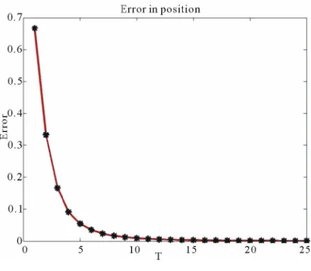
As a consequence of evaluating (12) in (15), the resul-tant diagonal terms are the ones of interest because they represent the mean-square errors of position and velocity. Since velocity affects position, we notice that good estimates of position are obtained only after obtaining good estimates for velocity. Figures 1
and 2 show actual versus predicted trajectories of a
translating object along X-axis and Y-axis, respectively.
Figures 3 and 4 depict the errors in position and speed,
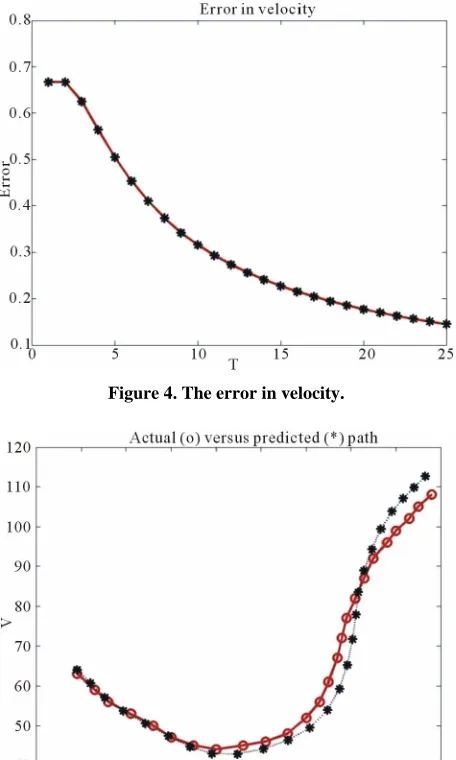
respectively. Figures 5 depicts the actual (o) versus
pre-dicted (*) trajectories of the moving object in 2D.
11 22
P k P k
2.2. Rotational Motion
[image:3.595.312.534.84.263.2]In general, a moving object undergoes a combination of translation and rotational motion. Therefore, a model for predicting rotational motion is necessary to complete the prediction model. Without loss of generality, we
[image:3.595.309.533.301.487.2]Figure 1. Actual vs. predicted trajectories of a translating object (point) along the X-axis.
[image:3.595.312.534.528.721.2]Figure 2. Actual vs. predicted trajectories of a translating object (point) along the Y-axis.
Figure 4. The error in velocity.
Figure 5. Actual (o) versus predicted (*) trajectories. represent a given moving object with its center of mass and some other reference (feature) points that be in the right place on the object. For example, a line segment in space is defined by its center of mass and its end-points. We only predict the trajectory of the center of mass and then relate the computations to the other reference points. Reference points are used to show the orientation of a given object. The mathematical analysis for developing the rotational-prediction model is analogous to the one of the translational case. Formally, let the orientation, of a rotating obstacle, Oi, be i and angular velocity i.
Using vector notation, it is:
i
ii
t t
t
(16)
If the sampling steps, of sensing the environment, are small enough then it is fair to assume that the angular acceleration of a rotating obstacle is constant
di orslowly changing. That is,
i d
i (17)
The analysis follows exactly as for the translational case. The resulting model can be used to predict orienta-tion around X and Y axes.
3. Prediction Algorithm
Table 1 describes the main steps in order to generate all
predicted configurations in 2D.
We integrate both prediction models introduced so far. To illustrate this procedure, we use an example. Suppose a line segment, represented by three points
1, cm,
a a a a3 is moving freely in a 3-D environment. We only predict the trajectory of center-of-mass point
acm that is regarded as a feature point. In view of thefact that we deal with rigid bodies, the prediction find-ings are applied to the other two end-points. The ex-pected orientation of the line segment at each new pre-dicted position is also computed. Using both the expected position and orientation, a point NA, that belongs to the
line segment at the current frame of center of mass ref-erence (N) is mapped to its corresponding position in the
global frame of reference (W). Formally,
1 1
W N
W N
A A
T
(18)
where is a 4 × 4 homogeneous transformation ma-trix defined as:
[image:4.595.309.539.478.729.2]W NT
Table 1. Algorithm 1.
Initialize P(0), x1(0) and x2(0) For i : 1 to No_of_obstacles do
For t=1 to N do
if t < 4 then
a=c
else
a=x(t‐1)‐2x(t‐2)+x(t‐3)
x1(t)=x1(t‐1)+x2(t‐1)+0.5*a
x2(t)=x2(t‐1)+a
P11=P11+P22+2P21
P21=P21+ P22
K(1)= 11
1 11
P
P
K(2)= 21
1 11
P
P
Z=Y(t)‐ x1 (t)
x1 (t)= x1 (t)+K(1)*Z
x2 (t)= x2 (t)+K(2)*Z
P22= P22‐K(2) P21
P21= P21‐K(2) P11
P11=(1‐K(1)) P11
Save predicted values and errors
Next t
13 11 12
23 21 22
31 32 33
0 0 0 1
x
y W
N
z
r d
r r
r d
r r
T
r r r d
The 3 × 3 sub-matrix
11 33
W
NR r r
, ,
represents the rotation matrix relating the current frame of reference (N)
to the global one (W), and d d dx y z denotes the dis-placement vector from the origin of N with respect to
frame W. We use the roll, pitch, yaw angles
representa-tion1 to describe the orientation of
N in W. Table 2
summarizes the steps required to predict the (n + 1)th
future position and orientation of a free moving object in space based on its first n positions and orientations:
4. Simulation Results
We presume a 2D environment in which an object is freely moving. Based on its past positions, configurations are estimated using the proposed model. The prediction is carried out over 25 sampling steps. Data points are arbitrary chosen.
In Figures 1-4, we predict the positions and
orienta-tions of the moving object that is specified with a center of mass and 3 feature points (vertices). The object trans-lates freely in 2D. Figures 1 and 2 show both the actual
sensed and the predicted trajectories of the object transla-tional motion in 2-D along X and Y axes, respectively. The errors between actual and predicted values in posi-tion and velocity are depicted in Figures 3 and 4,
[image:5.595.124.221.87.147.2]respec-tively. Note that the position error drops after the first observation is processed whereas the velocity error drops after the second observation. The mean square errors are 1.12 and 2.01 distance-units along X and Y axes, respec-tively. The predicted path is quite close to the actual tra-jectory as can be seen in Figure 5.
Table 2. Algorithm 2.
Input previous positions and orientations.
For i : 1 to No_of_obstacles do For each feature point Oi do
Using Algorithm 1,
1. predict next configuration: position
x , yp p
andorientation
θxp,θyp
.2. apply transformation and obtain the resulting
configuration.
Next
Next i
The effect of rotational motion of the same object is depicted in Figure 6. The mean square error is 0.369
radians (Figure 7). Figure 8 shows the actual and
pre-dicted trajectories for both translation and rotational mo-tion. The effect of rotation may be traced by tracking the symbols (*) and (+), which indicates the orientation (an-gle around X-axis). The details of this figure are already explained in the previous figures.
5. Conclusion
We have described a robust algorithm to predict futuris-tic configurations of a freely moving target in a time- varying environment. We employed the Kalman filter for tracking and motion prediction purposes for the reason that it is an effective and useful predictor-corrector esti-mator. It is optimal in the sense that it minimizes the es-
[image:5.595.310.538.537.718.2]Figure 6. Predicting rotational motion only for an object in 2D; orientation is indicated by the (+: actual) and (*: pre- dicted) symbols.
[image:5.595.56.281.541.730.2]Figure 7. Actual (o) and predicted (*) rotational motion. 1
[ , , ]
,
W
N XYZ x y z
x y x y z x z x y z x z
x y x y z x z x y z x z
y y z x z
R
c c c s c s c c s c s s
s c s s s c c s s c c s
s c s c c
Figure 8. Actual (solid) and predicted (dashes) configura
mated error covariance. The target motion is
uncon-[1] A. Basu and timizing Strategies
Bishop, “Improving Static and D
rd Arnold
ose, “Obstacle Avoidance in -tions of a moving object in 2D based on all previous figures. ti
strained. The ability of the proposed algorithm to embark on the prediction process from the first time step rather than waiting for few time steps is a noteworthy quality; no need to wait for few time steps as in the autoregres-sive-based systems. Simulation results confirmed the validity of the proposed model and demonstrated its the superiority. This research may be viewed as a seed point for further research in robot motion planning in a dy-namic environment.
REFERENCES
A. Elnagar, “Safety Op
for Local Path Planning in Dynamic Environments,” In-ternational Journal on Robotics Automation, Vol. 10, 1995, pp. 130-142.
[2] R. Azuma and G.
y-namic Registration in an Optical See-Through HMD,” SIGGRAPH 94 Conference Proceedings, ACM Press, Addison-Wesley, Orlando, 1994, pp. 197-204.
[3] S. Bozic, “Digital and Kalman Filtering,” Edwa Publishers, London, 1994.
[4] A. Chakravarthy and D. Gh a
Dynamic Environment: A Collision Cone Approach,” IEEE Transactions on SMC-Part A: Systems and Humans, Vol. 28, No. 5, 1998, pp. 562-574.
doi:10.1109/3468.709600
[5] C. Chang and K. Song, “Environment Prediction for a Mobile Robot in a Dynamic Environment,” IEEE Trans-actions on Robotics and Automation, Vol. 13, No. 6, 1997, pp. 862-872. doi:10.1109/70.650165
[6] A. Elnagar, “Prediction of Future Configurations of a Moving Target in a Time-Varying Environment Using an Autoregressive Model,” Journal of Intelligent Control and Automation, Vol. 2, No. 4, 2011, pp. 284 -292. doi:10.4236/ica.2011.24033
[7] A. Elnagar and K. Gupta, “Motion Prediction of Moving Objects Based on Autoregressive Model,” IEEE Transac-tions on SMC-Part 1: Systems and Humans, Vol. 28, No. 6, 1998, pp. 803-810. doi:10.1109/3468.725351
[8] P. Fiorini and Z. Shiller, “Time Optimal Trajectory
Plan-. Harrington and GPlan-. Pfeifer, “Constellation :
th-Velocity
Decomposi-ura and H. Samet, “Motion Planning in a
Dy-otion Planning—A ning in Dynamic Environments,” IEEE International Conference on Robotics and Automation, Vol. 2, 1996, pp. 1553-1558.
[9] E. Foxlin, M ™
A Wide-Range Wireless Motion-Tracking System for Augmented Reality and Virtual Set Applications,” In: M. F. Cohen, Ed., Computer Graphics (SIGGRAPH 98 Con-ference Proceedings,), Orlando, ACM Press, Addi-son-Wesley, 1998, pp. 371-378.
[10] T. Fraichard and C. Laugier, “Pa
tion Revisited and Applied to Dynamic Trajectory Plan-ning,” Proceedings of the IEEE International Conference on Robotics and Automation, Atlanta, 2-6 May 1993, pp. 40-45.
[11] K. Fujim
namic Environment,” Proceedings of the IEEE Interna-tional Conference on Robotics and Automation, Scotts-dale, 14-19 May 1989, pp. 324-330.
[12] Y. Hwang and N. Ahuja, “Gross M
Survey,” ACM Computing Surveys, Vol. 24, No. 3, 1992, pp. 219-291. doi:10.1145/136035.136037
[13] K. Intersense, “IS-900,” 2000. http://www.isense.com ry [14] K. Kant and S. W. Zucker, “Towards Efficient Trajecto
Planning: The Path-Velocity Decomposition,” The Inter-national Journal of Robotics Research, Vol. 5, No. 3, 1986, pp. 72-89. doi:10.1177/027836498600500304 [15] N. Kehtarnavaz and N. Griswold, “Establishing Collision
Zones for Obstacles Moving with Uncertainty,” Com-puter Vision, Graphics and Image Processing, Vol. 49, No. 1, 1990, pp. 95-103.
doi:10.1016/0734-189X(90)90165-R
[16] J.-C. Latombe, “Robot Motion Planning,” Kluwer
Aca-osh, “A Genetic-Fuzzy demic Publishers, London, 1991.
[17] K. Pratihar, D. Deb and A. Gh
Approach for Mobile Robot Navigation among Moving Obstacles,” International Journal of Approximate Rea-soning, Vol. 20, No. 2, 1999, pp. 145-172.
doi:10.1016/S0888-613X(98)10026-9
[18] R. Spense and S. Hutchinson, “An Integrated Architecture
back, K. Keller for Robot Motion Planning and Control in the Presence of Moving Obstacles with Unknown Trajectories,” IEEE Transactions on SMC, Vol. 25, No. 1, 1995, pp. 100-110. [19] T. Tsubouchi, K. Hiraoka, T. Naniwa and S. Arimoto, “A
Mobile Robot Navigation Scheme for an Environment with Multiple Moving Obstacles,” Proceedings of the IEEE/RSJ International Conference on Intelligent Robots, Raleigh, 7-10 July 1992, pp. 1791-1798.
[20] G. Welch, G. Bishop, L. Vicci, S. Brum
and D. Colucci, “High-Performance Wide-Area Optical Tracking—The HiBall Tracking System,” Presence: Teleoperators and Virtual Environments, Vol. 10, No. 1, 2001.