Embedded neural network design on the ZYBO FPGA for vision based object localization

(1)

1

Faculty of Electrical Engineering,

Mathematics & Computer Science

Embedded Neural Network Design

on the ZYBO FPGA

for Vision Based Object Localization

Konstantinos Fatseas

M.Sc. Thesis

July 2018

(2)

(3)

Abstract

During recent years we have been witnessing great advancements in the eld of computer vision due to the utilization of machine learning. Those achievements are attributed to the evolution of Convolutional Neural Networks (CNNs) as nowadays they are the basic building block of every state-of-the-art object de-tector and classier. There is an abundance of possible applications for CNNs and especially in cyber-physical systems, but the utilization of a CNN comes with a very high computation and memory requirements.

Therefore the objective of this work is to study the suitability of machine learning and more specically of a CNN in a visual servoing application. The application itself consists of two robots where one has the role of prey and the other of the predator. The CNN is dened as a classier and trained on a generated training dataset in order to avoid manual annotation. Then it is integrated into an object detection pipeline in order to extract the precise location of the prey robot. Furthermore, a pre-trained neural network is utilized so as to improve the overall performance of the object detection pipeline. Finally, an accelerator is developed in order to port the object detector into the ZYBO FPGA board and to meet the real-time constraint.

(4)

(5)

Acknowledgments

I would rst like to thank my supervisor Marco Bekooij. He consistently allowed this project to be my own work, but steered me in the right direction whenever I needed it. Furthermore, the proposed project was very challenging and gave me the opportunity to practice the hardware design skills I've acquired during my study in the Embedded Systems M.Sc. program. While, it also acted as a gentle introduction to the increasingly interesting eld of Machine Learning.

I would also like to thank all the colleagues that kept me company through-out my study. More specically, Viktorio, Oguz, Kiavash, Zhiyuan, Matheus, Stefano and Giovanni.

Finally, I must express my very profound gratitude to my parents Ineke and Yannis, and to my partner Nicoleta for providing me with unfailing support and continuous encouragement throughout my years of study. This accomplishment would not have been possible without them. Thank you.

(6)

(7)

List of Figures

1 Predator and prey robots . . . 2

2 The closed loop system developed by Moeys et al . . . 4

3 An articial neuron . . . 7

4 Example of an articial neural network . . . 8

5 Example of a training dataset . . . 10

6 Convolution example of a color image with a handcrafted kernel 11 7 An example of 2D convolution . . . 12

8 An example of 3D convolution with an RGB color image as input 13 9 Example of the ReLU activation function . . . 14

10 Some pooling examples . . . 15

11 The components of a typical convolutional neural network and an example of more a complex arrangement . . . 16

12 The Alexnet CNN . . . 17

13 An example of a residual learning block and of an inception module 18 14 R-CNN object detector pipeline . . . 20

15 YOLO object detector pipeline . . . 20

16 TPU block diagram . . . 21

17 Extraction of the GoPiGo robot . . . 24

18 Labeling of the dierent regions that the robot may lie within . . 24

19 Example of images created by the training dataset generation algorithm . . . 25

20 Accuracy comparison between various models . . . 30

21 Some of the architectures that were tested, in more detail . . . . 32

22 The feature maps generated by the intermediate convolution lay-ers of model C . . . 33

23 Another example of feature maps generated by the intermediate convolution layers of model C . . . 34

24 Yet another example of feature maps generated by the interme-diate convolution layers of model C . . . 35

25 Confusion matrix for models B, C and G . . . 36

26 The object detection pipeline . . . 38

27 Localization examples . . . 39

28 More localization examples . . . 40

29 MobileNets-based convolutional neural network . . . 42

30 MobileNets-based object detection pipeline . . . 43

31 Predator and prey robots together with the object tracking algo-rithm running at the background . . . 44

32 Samples of the CNN-based object detector's output . . . 44

33 The ZYBO Board . . . 45

34 Pixel reuse rate for a small input feature map . . . 49

35 The sliding window architecture . . . 50

36 The convolver module . . . 52

37 ReLU activation hardware . . . 52

38 Max pulling module . . . 53

39 Zero padding module . . . 54

40 Overall CNN accelerator . . . 56

(10)

42 Single and multi processing element implementation of the

accel-erator . . . 58

43 Data trac between a multi-convolver accelerator and the DDR SDRAM memory . . . 59

44 Structure description text le for model B . . . 60

45 The complete object tracking system . . . 61

(11)

List of Tables

1 A summary of the functions that the accelerator can support. . . 28

2 Topologies of the CNNs that were used for the accuracy compar-ison of gure 20 . . . 29

3 Computation of Model C's convolution part . . . 47

4 Computation of Model B's convolution part . . . 47

5 Total Resource Utilization . . . 64

(12)

Nomenclature

ANN Articial Neural Network

ASIC Application-Specic Integrated Circuit CNN Convolutional Neural Network

CPU Central Processing Unit DDR Double Data Rate DMA Direct Memory Access DNN Deep Neural Network DSP Digital Signal Processing FPGA Field-Programmable Gate Array FPS Frames Per Second

GPU Graphic Processing Unit IC Integrated Circuit

ILSVRC ImageNet Large Scale Visual Recognition Challenge RAM Random-Access Memory

ReLU Rectied Linear Unit

SDRAM Synchronous Dynamic Random-Access Memory SoC System on Chip

(13)

1 Introduction

During recent years we have been witnessing great advancements in the eld of computer vision due to the utilization of machine learning. More specically, image classication and object detection algorithms have been improved and are now delivering even super human accuracy in some tasks. The driving force has been the improvement of deep learning methods that led to the evolution of Convolutional Neural Networks (CNN). CNNs have been the core element of all the state-of-the-art image classiers and object detectors after the year 2012 when the winning method of the ImageNet Large Scale Visual Recognition Challenge [28] (ILSVRC) was based on a articial neural network for the rst time.

After the initial success of Krizhevsky et al.[16] at the 2012 ILSVRC, CNNs have been extensively studied resulting to an abundance of new tools, methods and applications. For this reason CNNs are nowadays a strong candidate for any task that involves computer vision like image based search on the Inter-net or autonomous cars where image sensors can provide information about the surroundings. Other areas that CNNs have been applied in order to achieve state-of-the-art performance include object tracking, semantic segmentation, pose estimation, text detection and recognition, scene labeling, image restora-tion etc. In fact, CNNs provide such a robust platform that they have been utilized in numerous applications even out of the eld of computer vision due to their ability to exploit correlations not only in the spatial domain but in the time and frequency domains as well. For example a CNN can be part of a system in areas like natural language processing, speech processing and speech synthesis.

The main advantage of machine learning is that it shifts the eort from the developing of application specic algorithms to the creation of a suitable training dataset for each task. On one hand, the collection of the training material and its annotation is a relatively simple task. On the other hand, the vast amount of examples that are usually needed require a lot of man-hours to be manually annotated. The importance of the training dataset is such that the spring of machine learning we are witnessing can be partially attributed to the compilation of large training datasets like the ImageNet that were not available in the past. The other two main reasons are the overall improvement of the training algorithms and the availability of Graphic Processing Units (GPUs) for general purpose computing.

1.1 Motivation

(14)

Figure 1: Predator (left) and prey (right) robots. The GoPro action camera which is mounted on top of the predator robot, is used to provide the input video stream.

case of wireless transmission. Furthermore, wireless data transmission requires excessive energy consumption, especially on a cellular network.

Applications like autonomous driving or industrial automation are subject to tight real-time constrain and low latency requirements, thus the solution of remote processing is not applicable in all cases. For real-time systems there is a need for reliable processing platforms that can provide guarantees about the execution time and also introduce low latency while being energy ecient. Meeting those requirements on platforms with limited resources is challenging but the availability of modern SoCs that include a portion of FPGA fabric lets us exploit the parallelism of CNN computation[22] and deliver enough computing power with a very good performance per watt ratio.

1.2 Problem Denition

The goal of this thesis has been the utilization of machine learning and more specically of a CNN in a visual servoing application. The application itself consists of two robots (gure 1) were one has the role of prey and the other of the predator, thus one robot (the predator) has to track the other and follow closely. Although initially the neural network was intended to take full control of the robot by being trained from end-to-end, after the involvement of a fellow student in the project it was decided to develop a more conventional control system. The controller would combine the output of the CNN with information about the ego motion by performing sensor fusion. As a result the CNN would be used only for tracking of the prey robot by using frames coming from a single image sensor.

(15)

core ARM processor together with FPGA fabric.

Furthermore, from the early stages of development it was known that the Raspberry Pi 3 board (which is already available on the prey-predator robots) is incapable of performing the amount of computation that state-of-the-art CNNs require in real-time. Additionally, in order to meet the real-time constrain with even a smaller CNN there was need for specialized performance-oriented software that would make use of the DSP capabilities of the ARM CPUs or of the VideoCore which is the equivalent of a GPU and is integrated into the BCM2837 SoC.

Those options were not taken into consideration due to the lack of scalability that such a specialized software solution would suer from. This is in contrast to the FPGA based SoC where the CNN computation can be accelerated on the FPGA thus leaving room for the control and navigation algorithm to run on the ARM cores. Finally, another issue of the Raspberry Pi is the latency that is introduced from the camera driver, this is completely omitted on the ZYBO board by synthesizing dedicated hardware for the image acquisition and using direct memory access (DMA) to directly save pixel values into the DDR SDRAM memory.

To summarize, the research question can be dened as follows:

Can a CNN be trained in order to act as a single-object detector, accelerated to meet the real-time constrain and integrated into an object tracking system on the ZYBO board ?

To answer the question, we need to brake it down into smaller objectives as such a system will require algorithmic, software and hardware development. Ad-ditionally, every step and decision taken will have consequences on the following steps. The objectives that arise from the research question are the following:

1. Create a training dataset suitable for this application

2. Research and evaluate existing CNN architectures 3. Develop a CNN based object detection algorithm

4. Dene a subset of functions to be used for the CNN that are suitable for acceleration from a complexity point of view

5. Develop software so as to study the underlying computation of the detec-tion algorithm and use as reference for the hardware implementadetec-tion

6. Realize a real-time object detection system on the ZYBO board

1.3 Related work

(16)

Figure 2: The closed loop system developed by Moeys et al.[21]

used in order to process color images of higher resolution coming from a stereo camera setup.

More recently, in 2016 Moeys et al.[21] in a very similar application (gure 2) to the one of this work, trained a CNN to make a robotic vehicle follow another one by relying only on visual information. Although, the work of Moeys provided a good starting point regarding the convolutional neural network architecture, there is a substantial dierence regarding the computing platform that was used. All the aforementioned studies rely on external stationary platforms for the computation of the neural network. In contrast to this project were the goal is to perform all the computation on-board on a small sized SoC FPGA board and in an energy ecient manner.

This brings us to the second part of this thesis, the hardware acceleration of the CNN. Because of the potential that vision based applications have, especially on embedded devices, there already exist numerous CNN accelerators. The existing accelerators target both ASICs and FPGAs as the rst can deliver sheer performance on high clock frequencies and be energy ecient but the later can be more exible and adapt to the CNN that is to be accelerated or to future architectures. ShiDianNao[3] and Eyeriss[2] are two of the ASIC CNN accelerators found in the literature. They are complex structures though, so it was unreasonable to base the design of this thesis's accelerator on those studies, mainly due to time limitation. There also exist a lot of accelerators for FPGAs but again the goal of those studies is to deliver state-of-the-art performance, resulting to complex architectures that are synthesized for high range FPGAs.

(17)

tools that are available at the moment.

This work is focusing on both the development of the CNN and its accel-erator. Therefor, it is necessary to extract useful features from the literature of both the deep learning and CNN acceleration domains and combine them in order to create a simple workow that will allow the training of small CNNs and its acceleration on the ZYBO board. The process of transferring the structure and the coecients to the embedded platform is also a challenging task but examples of this process can be found in studies like the Angel-Eye[8].

1.4 Contributions

Due to lack of experience on neural networks within the chair of Computer Architectures for Embedded Systems, this thesis mainly contributes as a start-ing point for further research on the topic and emphasizes on minimizstart-ing the computational cost and latency of the inference. For this reason the use of com-mercial frameworks or High-Level Synthesis is avoided and instead only open source libraries are used and the register-transfer level description is written with VHDL.

The points that this thesis contributes to can be specied as follows:

• Developing a method that can produce a large synthetic training dataset

with only a small number of actual images.

• Training of a relatively small convolutional neural network on the

automat-ically generated training set and compare it with existing architectures.

• Extracting the object's location by inspecting the output of the last

con-volutional layer in order to avoid complex algorithms with high computa-tional cost.

• Design and develop a re-congurable and lightweight CNN accelerator for

an FPGA that meets the real-time constrain and introduces acceptable latency.

• Integrate the accelerator into a SoC and develop the appropriate driver in

order to evaluate the accelerator and the neural network.

1.5 Report outline

In order to present the basic concepts that the reader needs to be aware, the 2nd Chapter provides general information on neural networks and presents some of the accelerators that have already been developed. Additionally, this chapter discusses the convolution operation as dened in the eld of computer vision and the other functions that can be used in feed-forward neural nets. Moreover the state of the art CNN based object detectors are presented and their advantages and drawbacks are discussed.

(18)

Chapter 4 documents the architecture that was developed and the reasoning behind the choices that were made throughout the process. Furthermore, the communication between the software and hardware is explained together. Fi-nally, the overall performance of the accelerator and of the convolutional neural network itself are discussed..

(19)

2 Background

Machine learning is a sub eld of Articial Intelligence and refers to computer systems that have the ability to learn how to solve a problem rather than being explicitly programmed to do so. Articial neural networks are only one of the approaches of machine learning, some of the other approaches are the Support Vector Machines, and data clustering.

Articial neural networks are computing systems loosely inspired by nature. A neuron in nature typically consists of the dendrites (Input connections), the main body and the axon (output connection). Its output is related to its inputs so a neuron can be thought as a system that receives, processes and transmits information. In a neural network like a brain, dierent kind of neurons intercon-nected with each other create a complex system capable of perceiving the world and exhibit intelligence. This is a simplication though, because the human brain for example is far more complex. It is still unknown what is the exact functionality of a neuron and how exactly they contribute in this high form of intelligence that a human can display.

2.1 Articial Neural Networks

A simple neuron in mathematics will have a set ofninputs,(x1,x2, ..., xn)and

a single output y. The neuron then has to learn a set on n weights, each of

them will be multiplied with the corresponding input and the sum of the results will be the output. Thus, the functionality of a simple articial neuron can be described as a function f(x, w) = x1w1+x2w2+...+xnwn. Being a linear

function though, such a simple neuron cannot form networks that are able to be trained to solve dicult problems. The solution to this is to add an extra activation function that will havef(x, w)as an input and will calculate output

yin a non-linear fashion, some of the most commonly used non-linear functions

will be introduced in section 2.2. The structure of such an articial neuron can be seen in gure 3. First the sum of the weighted inputs is calculated and then the so called transfer function or activation function will produce the corresponding output of the neuron.

(20)

[image:20.595.234.422.128.317.2]

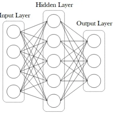
Figure 4: Example of an articial neural network (ANN) and more specically of a deep neural network as between the input and output layer is also a hidden one. An ANN is an interconnected group of nodes like the one depicted at gure 1. Information ows towards one direction (input→output) in a feed-forward

network like this one.

2.1.1 Neural Network Topology

By using the articial neurons as basic structure elements we can now arrange them so that multiple neurons are interconnected and form what is called a deep feedforward network, such a topology is depicted in gure 4. The neurons are grouped in layers where a neuron's inputs is connected to the outputs of all the neurons that the previous layer has, such an arrangement is called a densely or fully connected network.

A deep feedforward network may have 3 or more layers, the rst layer is directly connected to the input and the last layer is the output of the network, the layers in between are called hidden layers. The basic property of this type of network is that the information ows from the input towards the output without any feedback loop. Furthermore, the neurons do not have any connection with other neurons of the same layer. Those properties are important when it comes to hardware design because they allow a great degree of parallelism as shown in chapter 4.

(21)

2.1.2 Training of Neural Networks

The success of neural networks derives from the ability to gradually learn how to solve a given task by being trained. Training is the procedure of setting the correct values to every neuron's weight set so that the nal output of the network approximates the desired response as close as possible.

Throughout this project the training methods were not investigated and by using a machine learning library the underlying training algorithms are hidden as the neural network development is done in a higher level of abstraction. Although there is no demand for a machine learning practitioner to be fully aware of the training procedure, some basic concepts need to be explain due to the fact that we still lack of standardized method to chose a network architecture for a given task.

Neural nets can be used for classication which is to classify a given input into one of a nite amount of categories that the network has been trained against. Another option is to use the network for regression, in this case the output can be within a range of continuous values. Figure 5 shows a simple example of a training dataset that can be used in order to extract the location of a shape from an image. Although the example is trivial and it is easy to extract the location with a traditional algorithmic approach, it can be seen that the same problem can be tackled with both classication and regression.

In general, we use classication when the output takes discrete values or we have a number of classes from which we want to pick one. For example, if we wanted a neural network to predict the number of cars in an image, we would use a classier whose output neurons will correspond to the discrete values 1, 2, 3 etc. On the other hand, if the task is to predict the future value of a stock or commodity, the output would be a single neuron whose activation can be any value.

In the case of gure 5, a classier would have 3 neurons at the output layer where the one with the highest value would indicate in which part of the image is the shape located. In contrast, by using regression the network can be trained to predict the position of the shape by indicating a specic pixel index with a single neuron at the output layer.

Another important aspect of a neural network is its capacity. Capacity is called the maximum complexity of the function that the network can t. It is closely related with the topology and the size of the network, a network with 2 hidden layers and 20 neurons for example has less capacity that a network with 200 neurons and 4 hidden layers. This is a very rough explanation but sucient to let us introduce the problems of over-tting and under-tting of a neural net. Given a training dataset, a neural network will under-t if the architecture and number of neurons that were chosen is simply not enough to learn how to solve the problem, namely how to map the training set inputs to the desired output. On the contrary, if the network's capacity is much higher than the capacity that the problem requires, the network will be over-trained and will subsequently fail to generalize and work on previously unseen data.

(22)

Figure 5: Example of a training dataset. This dataset could be used in order to detect the position of an object in an image. On the left, the dataset is structured in a way that allows us to use a classication network. By dividing the image into multiple segments we can train the network to predict in which of those segments is the object located, in the example we use three but the number of segments can be vary. The label in this case is an integer that points to the segment that the object is. On the right side the dataset is oriented into solving the same problem with regression. This time the label is a decimal value that can be directly translated into a specic pixel coordinate along the horizontal axis. Those two ways of formulating the same problem will have consequences on the architecture of the networks that could be used for those two examples. In the case of classication the neural network's output layer will consist of three neurons whose value will indicate the probability that the object lays into the corresponding segment. On the other hand, if regression is used then the output layer will consist of only one neuron whose output value will directly indicate the position of the object.

moment that the network operates on new images, dierent from the training set, it will fail to locate the shape.

To conclude, training is the process of tuning the parameters of a neural network which are usually carefully initialized so they do not introduce any bias. The purpose of the training is to create a neural network that will be able to generalize on a problem by only learning on a limited amount of examples. It has been proven that the bigger the size of the training set, the better the network generalizes on new data. However, training dataset generation is a time-consuming process as it usually requires humans to manually annotate the dataset. Usually a training set for computer vision will consist of millions of images that will come together with a vector with size equal to the number of images and will indicate the class of every image as a number. Some extensively used training sets are ImageNet, PASCAL and COCO[28, 4, 18].

(23)

2.2 Convolutional Neural Networks

A fully connected neural network is powerful enough to tackle a wide range of problems but will require an enormous amount of parameters when it comes to computer vision problems. To illustrate this problem the MNIST database can be used as an example of a computer vision task that has to do with hand writing recognition. The database consist of 60000 training samples and 10000 testing samples where every sample is a grayscale image of size 28×28pixels

containing one handwritten digit. If a neural network with a rst layer that contains only 40 neurons is used it will result to a high number of weights which is equal to28×28×40 = 31360, that is because every neuron will be connected

to every pixel of the input image. The aforementioned amount of neurons is very small compared to the size of a neural network designed for computer vision. So, eventually the amount of memory needed to store the parameters will become the bottleneck of the system.

The number of parameters can be reduced if a weight sharing technique is applied. Convolutional neural networks are the most successful type of deep feedforward network in practice and they show remarkable results in dataset with strong spatial relation like images and sound recordings. They use small kernels (as dened in image processing eld) in order to reduce the amount of parameters but the idea itself is not new. In traditional computer vision convolution of an image and a kernel is used in feature extraction where by applying a mask over the image it is possible to extract information about the edges for example.

In the past feature extraction was used as a rst step to extract information about the content of an image and then pass it to an SVM in order to classify the content by using the extracted features. LeCun et al.[17] show how the hand writing digit recognition problem can be solved with a convolutional neural network, note that the study was published 20 years ago. Conv nets were never utilized widely only until recently, mainly due to some newly developed algorithms [6] that made training for big datasets feasible and because GPUs provide now the computation power that is needed for the training procedure.

Convolutional neural networks consist of a number of convolution layers and usually a smaller number of fully connected layers on top of them that produce the nal output of the network. This is similar to the traditional approach with

Figure 6: Convolution example of a color image with a3×3handcrafted kernel,

(24)

[image:24.595.232.410.125.312.2]

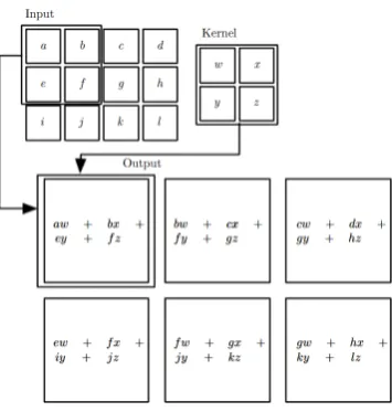
Figure 7: An example of 2D convolution. We perform 'valid' convolution as the output is restricted to only positions that the kernel lies entirely within the image. The number of pixels that the kernel is moving in order to calculate the next output value is called stride. In this example the stride of the convolution is one as the kernel moves one pixel every time. Illustration from [7]

the future extraction and an SVM on top but they dier because instead of hand crafted kernels, now the whole network is trainable from end-to-end and the all the parameters are subjected to the training algorithm.

Another function that is introduced in ConvNets is pooling. Pooling is when we sub-sample the result of a convolutional layer before it is forwarded to the input of the next layer. As a result it further reduces the amount of computation as it basically reduces the number of neurons without limiting its capacity. Pooling will be discussed in more detail in part 2.2.3.

2.2.1 The Convolution Operation

Convolution is a mathematical operation that can be applied on two functions and create a third one that will be a modied version of one of the functions. Under the scope of neural networks and image processing in general, convolution is the cross-correlation between an input multidimensional matrix and a smaller matrix (the kernel) of equal dimensions. The following equation describes the convolution of a two dimensional feature map I and the two dimensional kernel K. i and j are the width and height of the input and m,n are the width and height of the kernel.

S(i, j) = (I∗K)(i, j) =X m

X

n

I(i+m, j+n)K(m, n) (1)

(25)

[image:25.595.146.397.127.348.2]

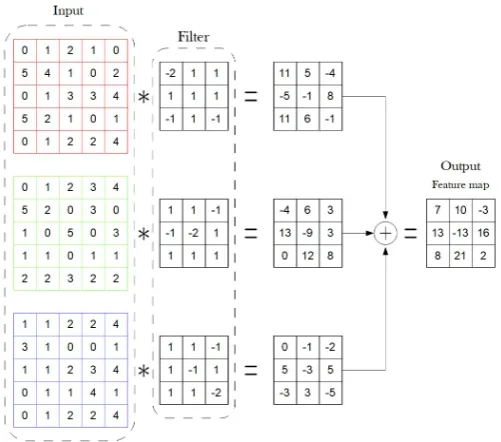
Figure 8: An example of 3D convolution with an RGB color image as input. As in gure 7 we perform a 'valid' convolution, thus the output is smaller than the input, in this case from an input of 5×5 pixels we get a 3×3 feature

map. In general if 'valid' convolution is used then the output size is equal to

Input Size−Kernel Size+ 1and this applies for both the width and height.

a 2D matrix which is similar to 3 or only one feature map. Figure 8 illustrates a convolution of a small input example that represents an RGB image with a simple lter with3×3kernels.

In the case of convolutional neural networks, each element of the resulting feature map can be thought as a separate neuron. Those neurons are the result of applying on the input the same kernel, thus we achieve weight sharing by using only a small number of weights that are shared among all the neurons that constitute a feature map.

2.2.2 Activation Functions

Although the main component of a convolutional neural network is the con-volutional operation, there is still need for non-linear components in order to give the ability to the network to approximate complex functions. In this part some of the commonly used functions are listed. The use of these activation functions is not limited only to ConvNets but can also be used in traditional neural networks.

• The Logistic function is a commonly usedSshaped function which belongs

to the Sigmoid functions family. It has the property to limit the output in between two horizontal asymptotes as the input value approaches innity. The function's equation is the following:

f(x) = 1 1 +e−x =

ex

(26)

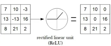
• ReLU is an abbreviation for rectier linear unit, it turned out to be one of

the most successful and widely used activation function. Basically it only lets positive values to propagate through the network and sets all negative values to zero. Thus, its equation is:

f(x) =x+ =max(0, x) (3)

• The Softmax function is a special case, its an activation function that is

mostly used as the very last component of a classication neural network. The reason is that it has the ability to map an arbitrary vector into an equal sized vector that contains values between zero and one that have a sum of one. This is very useful as those values can be interpreted as a probability distribution over the possible classes. In the following equation K is the number of elements (classes) of the vectorσv.

σ:RK →(0,1)K σ(zj) = e

zj

PK

k=1ezk

f or j= 1, . . . , K (4)

[image:26.595.231.416.487.564.2]

The aforementioned functions are some of the most frequently used but the list is not exhaustive as there exist many other functions with dierent properties and advantages. Because of the research that is still ongoing on the eld of deep neural networks, new ideas and components are proposed by researchers constantly.

Figure 9: Example of the ReLU activation function. The input to the function is the example convolution's output of gure 8. The functionality is simple as all the positive values remain the same whereas all negative values are replaced by zero.

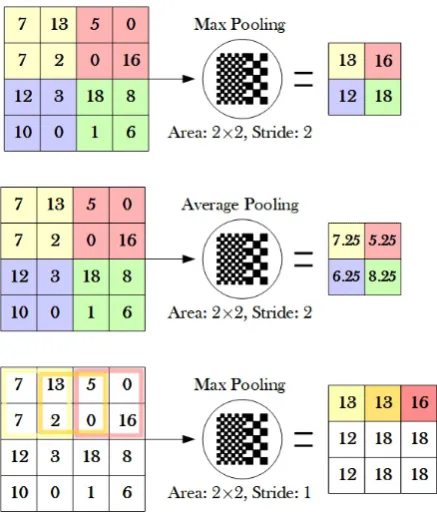
2.2.3 Pooling

(27)

[image:27.595.162.381.128.386.2]

Figure 10: Some pooling examples. The two upper examples show the result of max and average pooling over an area of 2×2 and with stride 2, the area

from which the resulting value is extracted and the value itself have the same background color. The last example at the bottom of the gure depicts a max pool over the same area as before but with stride 1. This time the output has bigger dimensions as the areas now overlap due to the smaller stride, this is also the reason that we don't use background colors but instead we use only a few boxes for clarity.

depicts max and average pooling which are the most used among convolutional ConvNets. As their name suggests, in the case of max pooling we extract the maximum value of an area whereas in the case of average pooling we calculate the average value of the area.

It is important to note that depending on the objective of the CNN it may be benecial to choose average pooling over max pooling due to its property to preserve the location of a feature in a better way, thus giving better results when localization of an object is needed. On the contrary, average pooling will require more computation in order to calculate the average value of an area than max pooling which only extracts the maximum.

2.2.4 Convolutional Neural Networks for Classication

(28)

Figure 11: The components of a typical convolutional neural network (left and center) and an example of more a complex arrangement (right). In some cases a convolutional layer is viewed as a convolution followed by an activation function and sub-sampling (Left). More recently though, due to the number of complex architectures that have been proposed, this terminology is not used often. In the most common terminology every stage is regarded as a separate layer (cen-ter), in this way we can more easily describe network architectures like the one shown at the right part of this gure where pooling is not applied after every activation (detection layer). This illustration was inspired by gure 9.7 of the Deep Learning book[7].

by the non-linear activation and the pooling operation, the convolution →

activation→pooling arrangement is usually called a convolutional layer.

An-other common arrangement is the stacking of multiple convolution-activation blocks before the pooling operation. Some of the state-of-art networks that will be presented in this part make use of this topology.

• Alexnet[16] was the rst neural network to win the ImageNet competition

back in 2012. Developed by Alex Krizhevsky et al. it was based on the rst ever convolutional network we previously discussed, namely the LeNet, introduced by LeCun et al. at 1998. Although from an architectural point of view they are very similar it was the availability of GPUs for general computing that made the training of such a network feasible for a multi class classication problem by training against millions of annotated images.

• VGG[31] is a family of ConvNets developed by the Visual Geometry

(29)

Figure 12: The Alexnet CNN[16]. It consists of 5 convolution and 3 fully con-nected layers. The network has two branches because it was trained on two separate GPUs, one branch on each GPU. With the use of newer libraries there is no reason to split a network into dierent parts. Note that the rst convolu-tion layer consists of kernels with dimensions of11×11, the second of5×5,and

the rest of3×3.

AlexNet and VGG are CNNs with relatively simple structure because the layers are stacked after each other and data ows in one path. In the following years after their initial success it became obvious that deeper networks are not necessarily more accurate so new techniques were introduced in order to increase the capacity of the networks but not limit their train-ability which was the main issue with very deep architectures. The problem is that during the back-propagation process the very rst layers of a deep network will not be suciently trained (vanishing gradient problem) so there was need for developing new ways that will allow even deeper network to achieve state-of-the-art accuracy.

The solution is to make wider architectures, not only deeper and to allow layers to get as an input not only the output of the one previous layer but rather have as an input information from multiple previous layers. The networks that are listed bellow are noteworthy as they introduced some very interesting ideas. With those ideas it was possible to lower the classication and detection errors even further and reduce the overall size of the networks as well. This means that by using more sophisticated and complex architectures, the number of parameters of a network can be reduced without an accuracy penalty.

• ResNet[9] was a groundbreaking network as it introduced the idea of

(30)

Figure 13: An example of a residual learning block (left) and of an inception module (right). Both architectures help the training process of deeper networks. A rough explanation of how this is achieved, is that the training algorithm has the ability to chose the path that conveys more useful features or even combine them with features of previous layers.

a number which is much smaller from the VGG ConvNets for example.

• Inception V4[32] is yet another interesting network from an architectural

point of view. With this convolutional network Szegedy et al. introduce an other module that is used in order to produce features from various sized kernels (1×1,3×3and5×5convolutions) in every layer and then

concatenating the result before it is fed to the next layer.

• MobileNets[10] are a family of neural networks (developed by Google's

engineers) that targets mobile devices with limited resources. It has the ability to be congured according to the user's needs. The depth and the number of parameters of the network can be decreased if the target platform is not powerful enough to cope with the full network. What make MobileNets to require less computation than the previous networks, is the use of point wise convolutions (1×1 kernel) in order to create a

more compact representation of the features that are being extracted with

3×3 convolutions. A version of the MobileNets was used for the object

detector and proved to be very robust in the single-object detection task, this is further discussed in Chapter 3.

(31)

environment. On the other hand, reusing such a network will require an accel-erator capable of performing the required computation. In the following part we introduce some of the object detection techniques that have been based on CNNs.

2.3 State-of-the-art CNN Based Object Detectors

After the initial success of CNNs for classication it was natural to use them for the task of object detection as well. In classication challenges the goal is to predict which is the main objects of an image. Usually, the object covers a large area of the image and is in the center. On the other hand, detection is the task where we predict which objects lie within the image and furthermore specify their locations. This makes the CNNs trained for the Imagenet classication challenge not directly useful for detection.

The initial approach to bridge the gap, was to extract areas of the image with a sliding window of various scales and evaluate the result of the classier. This approach requires an enormous amount of computation and does not oer real-time performance due to the multiple evaluations of the CNN. Another approach is to pre-process the extracted areas and list them based on the probability that they include an object. After the selection of the most prominent areas the CNN is evaluated only on those and not all the initially extracted areas. This method is minimizing the computational burden but not enough in order to make it suitable for real-time systems.

Convolutions have the property to preserve information about the location of the features that are being extracted so the next generation of object de-tectors make use of this property by training the network to directly predict bounding boxes. The following CNN based object detectors represent the two aforementioned methods and are worth our consideration for the object detector that has to be developed.

• Region-based CNN (R-CNN)[5] is a very well known object detector that

(32)

Figure 14: R-CNN object detector pipeline[5]. The rst step is the extraction of regions that have the higher probability to contain an object, after the selec-tion those regions are resized to t the classicaselec-tion CNN and then evaluated. Finally, the results of the evaluations are combined in order to create bounding boxes around the detected objects.

• YOLO[27] is a object detector which treats detection as a regression

prob-lem in one single CNN that outputs bounding boxes and class probabil-ities. This is done by segmenting the image into multiple areas, where each area can contain a xed amount of bounding boxes. For each box of each region, the output layer will predict a pair of coordinates (x, y) for

the center of the box, its width and height(w, h)and a condence value.

Furthermore, for each area the neural network makes a class prediction. The last layer's output vector has a length of A×(B×5 +C), whereA

is the number of areas, B is the number of boxes per area and C is the

number of classes that the CNN can classify. Note that B is multiplied

by5as each box has5 variables(x, y, h, w, conf idence). The nal step is

to combine the predicted boxes and classes of each area in order to create the nal result . By evaluating the CNN only once there is a big benet regarding the computation which is required, so YOLO is the most promi-nent candidate for real-time systems. This approach has been proved to deliver robust results, comparable with the region based detectors but its much faster. Lately, more and more object detectors are based on similar methods which extract the location of the objects directly through the convolutional layers.

(33)

[image:33.595.129.414.127.336.2]

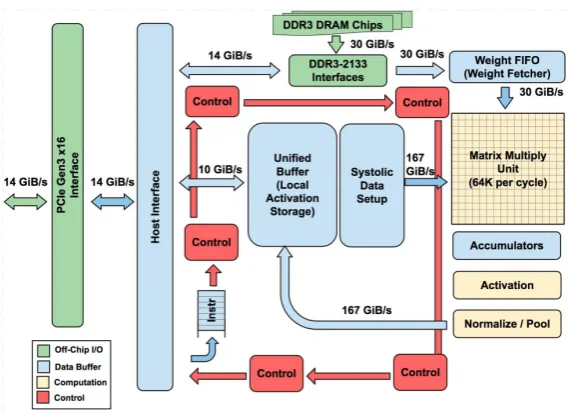
Figure 16: TPU block diagram [14]. Note that most of the components serve as data buers due to the very high demand for local memory in neural network accelerators. The core of the system is the matrix multiply unit and everything is built around it in order to fetch the parameters and the data but also to write back the result.

2.4 Convolutional Neural Network Accelerators

The rapid development of convolutional neural networks in the recent years is also attributed to the introduction of GPUs into general purpose computing. Of course big training datasets and new training methods along side new ar-chitectures played a signicant role as well, but in absence of sheer computing power those achievements would not be available to everybody.

In this part we discuss some of the hardware architectures that are designed to accelerate the training and the inference of neural nets. In general such specialized hardware can be faster and is more energy ecient than the GPUs, CPUs on the other hand are not the optimal platform in any way for neural networks, as they fail to exploit the parallelism that exists in neural network computation.

Although researchers published some very specialized hardware for ASICs and FPGAs, it is be noted that big tech companies nowadays are behind many of the recent achievements and also provide a lot of open sourced tools and training sets. The same companies will usually oer cloud computing platforms in order to make the usage of their software possible even in less capable devices like the Raspberry Pi 3. In the case of an computer vision application for example, the image would be acquired from the camera and then transmitted to the cloud platform, the computation will take place in the data-center and only the answer will be transmitted back to the embedded device.

(34)

training phase, the second version that was recently announced will be able to do both inference and training. In gure 16 illustrates the block diagram of the TPU, it can be seen that the basic block of the device is the matrix multiplication unit which performs the convolutions. A signicant amount of area is dedicated to the connection of the computing blocks to the weights and data memory but most of the area is allocated for the internal buers and the matrix multiply unit.

(35)

3 CNN based Object Detection

This part documents the development of a suitable training dataset for the prey - predator application and the training procedure of the CNN together. We also show the results we got from the dierent classication architectures that were tested. Furthermore, it is shown that those architectures are suitable for basic object detection and this can be further improved if we combine our neural networks with a pre-trained CNN.

Due to the iterative development, all the components of the work were re-designed and evaluated multiple times, especially due to the close relation of the CNN functionality and the accelerator. Here, presented is only the nal state of the development

3.1 Training Dataset Generation

An articial neural network training may be unsupervised or supervised. The former means that we dene a cost function and we let the back-propagation algorithm minimize the cost by working on the task without any previous knowl-edge or example. During supervised learning on the other hand, we also dene a cost function but now we rst provide examples of the desired output and we hope that the network will imitate the behavior on new inputs as well. For this thesis we train the CNN in a supervised fashion as this is the common case in literature for image classication and has been proven to deliver good results, whereas unsupervised learning is more challenging to apply.

In order to perform supervised training there is need for a big number of examples in order to tune the parameters for maximum performance on unseen data. Moeys et al. created a training dataset of 500.000 examples by recording 1.2 hours of video and manually annotating each frame to indicate the ground truth position. The video recordings were acquired directly from the image sensor of the robot which was remotely controlled for this purpose. In this thesis there was no constraint on the environment that the robots could operate so the goal was to be able to detect the robot in any environment. This rises the demand for an even bigger training dataset that will include many and also diverse examples. Additionally, at the beginning of the project the image source was not specied so the option of recording video from the robot itself was not available.

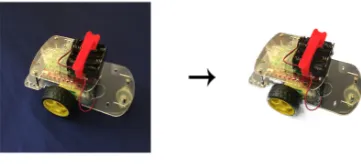
To overcome those issues so as to quickly start experimenting, it was decided to create an articial dataset by using a small number of images from the robot in combination with a larger number of random background images. In order to have the GoPiGo in various poses that we can combine with the dierent backgrounds, it was rst needed to extract only the robot like in gure 17 . Then we save it in an le format that can also include transparency information, in this case the PNG le format was selected.

(36)

[image:36.595.229.410.133.215.2]

Figure 17: Extraction of the GoPiGo robot. It can be seen that the extracted picture of the robot is inuenced by the environment due to the transparent material that it is made from and furthermore, by the lighting conditions as well.

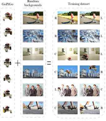
help the network to not correlate the GoPiGo with features that can also be extracted from other objects as well. To make the dataset even more versatile, the robot's pictures are randomly resized and rotated in addition to altering the color and lighting properties of the generated image. Some of the images used are shown in gure 19 together with samples of the generated training images and the corresponding label. The generated images are in most cases unrealistic but that is not a disadvantage as we want to extract features that do not correlate with the context of a scene.

Figure 18: Labeling of the dierent regions that the robot may lie within. L, C, R are for the left, central and right part of the image whereas N indicates the absence of the robot. The dimensions of the images we used to train of our CNNs are160×120pixels.

[image:36.595.232.416.407.526.2]

(37)

[image:37.595.103.443.190.577.2]

(38)

the absence of the robot we need a fourth class, this means that the classier will be trained to classify each frame into those four categories. Finally, for better results during the training phase it is benecial to have an equal number for examples per class, so each category (Left, Center, Right, Non-visible) should be represented ideally by 25% of the images in the training dataset.

It was chosen to follow this method (LCRN) which was found in the work of Moeys et al. The reason is that the initial approach to the problem was to train a network from end-to-end, thus the output of the network would directly drive the robot. This is the simplest way to tackle the predator - prey problem but is not optimal due to the inability of this simple solution to preserve information from the past frames. However this method was proven to be a good starting point and the classication networks that were trained with this training dataset were also used in for localization as we discuss in part 3 of this Chapter.

3.2 Training a Simple CNN

The availability of the training dataset lets us move to the next objective of this part which is the training of a CNN on this classication problem. It was decided to perform the training procedure oine. This is to dene and train the neural network on a workstation rather that the ZYBO board itself. Similar to the development of software for embedded platforms which is done on a workstation. The training procedure of a CNN is a very heavy workload due to the large number of CNN evaluations that need to be done, thus it is convenient and in some cases unavoidable to train the ConvNet on a workstation.

In this part, the terms architecture, topology and structure of a CNN, all refer to the specic way that the layers are arranged. The term model on the other hand, is used to describe both a CNN architecture and the trained weights that constitute its kernels and neurons in general.

3.2.1 Tools

Due to the even growing interest in machine learning recently, there is an abun-dance of tools that somebody can use in order to train and use ConvNets. As mentioned previously, the big tech companies like Microsoft, Amazon and Google were the rst to utilize machine learning for commercial applications. This led them to develop tools that were rstly used internally but later were given to the public as well. Tensorow[1] for example was published by the Google Brain team as an open source library in 2015 and is currently used by many machine learning practitioners. It provides APIs in many programming languages and also supports the use of NVIDIA's GPU's for parallel comput-ing. Big companies do not directly prot by the tools they develop as they are mostly open sourced. As we discussed in part 4 of the previous chapter though, they oer the possibility to accelerate on their cloud computing platforms the training phase or even the inference in case of an embedded device and those services are not for free.

(39)

and maintained by researchers of the Berkeley University.

For this thesis we make use of the Tensorow library but not directly. The reason is that Tensorow is regarded as a low-level library and requires the user to have some prior knowledge on the training algorithms. This was not the case for this project, so the Keras library was used on top of Tensorow in order to simplify the training process.

Keras is an open source library for Python which has the advantage of being well documented and constantly maintained by its developers. Thus, it oers a friendly environment for inexperienced machine learning practitioners by hiding a lot of the complexity that Tensorow needs in order to set up the training algorithm and tune its parameters. As Keras is simply an interface between the user and the computation libraries, it can be used with Tensorow, MXNet, Microsoft's CNTK and Theano as well.

3.2.2 Hardware Design Considerations

After the initial trials on CNN training, it became apparent that we should de-ne a small set of supported functions due to the multitude of options that are available. Because the nal goal of the thesis was to accelerate the CNN compu-tation on the resource limited ZYBO board, it would have been very ambitious to start the development of a fully exible architecture which would support all the available functions and their variations. Those restrictions though, apply only to the convolutional part of the networks. This is because the computation of the fully connected layers at the end of the network can be handled by the ARM cores of the Zynq SoC. Thus, more complex functions can be performed by writing C code.

In order to dene this sub-set of supported functions we take into considera-tion how commonly they are used in general and the diculty of implementing them on an FPGA. In the case of the convolution which is the basic block of every CNN, the decision was to constrain the kernel size to only3×3 with a

stride of 1 pixel like the example in gure 8 . This convolution conguration is the most commonly used among the state-of-the-art ConvNets and in some cases like the VGG CNN, it is the only one.

This is in contrast to the Inception CNN that utilizes convolutions with various kernel sizes for example. As a consequence to this decision, many of the state-of-the-art CNN will not be able to be accelerated. However, on the other hand the design of the convolver becomes easier due to the absence of a sophisticated interconnection network between the multipliers that would have been required if we had to support multiple kernel sizes.

The pooling function was decided to only extract the maximum value from an area of2×2with a stride of 2pixels, similar to the upper example of gure

2.2.3. The reason behind this decision is again the fact that this variation is the most commonly used and furthermore it usually results to feature maps with even dimensions which is convenient and requires simpler controller on the FPGA. Usually, the width and height of images acquired from cameras have a ratio of4/3, for example640×480 or 1024×768 are common resolutions for

small size images. By using this variation of the pooling function the result after sub-sumpling a640×480feature map will have dimensions of 320×240

which are again even and eventually easier to handle.

(40)

Function Convolution

Activation Pooling

Restrictions

Kernel size: 3×3, Stride: 1, Zero padding: optional

ReLU only

Area size: 2×2, Stride: 2

Table 1: A summary of the functions that the accelerator can support.

the feature maps before the convolution stage. Because convolution will always reduce the size of the output as explained in gure 7 . It is possible to keep the output dimensions similar to the input's if we rst add zeros around the input feature map. This type of convolution is called same usually. For example, if convolution is performed on a640×480feature map, it will result to an output

with dimension of 638×478. By using zero padding we rst increase the size

of the input to642×482and then we perform the convolution which will bring

back the dimensions to the original640×480.

Finally, the activation allowed on the convolutional part of the CNN is only ReLU and this is due to the simplicity of implementing the hardware to perform this activation. ReLU lets all positive values pass and only sets all negative values to 0. In hardware the sign of a value is described in a single bit, where logical 1 indicates a negative value and 0 indicates that the value is positive. Thus, ReLU can be implemented by only driving a multiplexer with the sign bit which is very fast and cheap regarding the resources needed. Luckily, ReLU is the mostly used activation and delivers good performance during training as well.

3.2.3 The Architectures

Inspired by the work of Moeys et al. the architectures dened for our problem are very similar to the ones that they have tested for their application. By obeying to the restrictions as listed in table 1, we specify similar architectures for our CNN. In contrast to their work, those shallow architectures do not achieve high accuracy on our training dataset though.

An explanation may be that our training dataset is more complex due to the random backgrounds we use. Additionally, they blend the input image with information from a Dynamic Vision Sensor. Therefore, there is a substantial dierence between the dataset they used and ours. However, eventually we were able to achieve higher accuracy by specifying deeper neural networks with more than two convolution layers.

The training dataset consists of 38000 samples and we use another 2000 samples for evaluation. The total number of 40000 images was the upper limit due to the RAM usage of the Keras library which for this number of samples is 10GB. This amount of RAM is needed because instead of using 8bit integer values for the pixels, we have to scale them in between 0 and 1 which requires the usage of oating point values of 32bits. This is due to the faster convergence that we achieve during the training procedure.

(41)

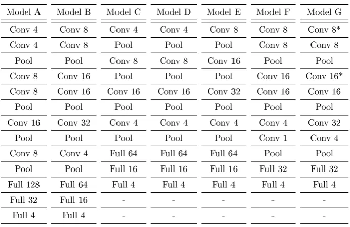
Model A Conv 4 Conv 4 Pool Conv 8 Conv 8 Pool Conv 16 Pool Conv 8 Pool Full 128 Full 32 Full 4 Model B Conv 8 Conv 8 Pool Conv 16 Conv 16 Pool Conv 32 Pool Conv 4 Pool Full 64 Full 16 Full 4 Model C Conv 4 Pool Conv 8 Pool Conv 16 Pool Conv 4 Pool Full 64 Full 16 Full 4 -Model D Conv 4 Pool Conv 8 Pool Conv 16 Pool Conv 4 Pool Full 64 Full 16 Full 4 -Model E Conv 8 Pool Conv 16 Pool Conv 32 Pool Conv 4 Pool Full 64 Full 16 Full 4 -Model F Conv 8 Conv 8 Pool Conv 16 Conv 16 Pool Conv 4 Conv 1 Pool Full 32 Full 4 -Model G Conv 8* Conv 8 Pool Conv 16* Conv 16 Pool Conv 32 Conv 4 Pool Full 32 Full 4

-Table 2: Topologies of the CNNs that were used for the accuracy comparison of gure 20. All the models are simple feed-forward structures without any branch or feed-back loop. The rst layer is the one at the top of each column while the last layer is always the fully connected layer (Full 4) at the bottom. Thus, the ow is from the top to the bottom of each column. The asterisks (*) at model G convolution layers indicate the absence of an activation function directly after the convolution. In any other case of this table, the convolutional layers are always followed by a ReLU and the fully connected layers by sigmoid or softmax activation. Furthermore, the number next to the Conv indicator is how many lters are applied on the specic convolution layer. The rest of the parameters of each layers follow the rules as dened in table 1.

was used is 'adam'[15] together with 'categorical crossentropy' as the loss func-tion. The result of the training procedure of some example models are shown in gure 20 while the structure of each model is described in table 2.

Although the accuracy that the models achieve during training is very high, the networks do not perform so well when evaluated on new images coming from a webcam or a mobile phone. The main issue is the big number of false positives. This is when the GoPiGo robot is not in the image but the network predicts that it is left (L), right (R) or in the center (C) instead of the correct non-visible (N) class. In this case we call predicted class the one that had the biggest probability, so it might be that in some cases the network is not strongly suggesting a wrong class but we treat this as a misclassication.

[image:41.595.99.445.122.347.2]

(42)

Figure 20: Accuracy comparison between various models. The trend we observe is that topologies with more convolutional layers perform better on the generated training dataset.

more red objects which led to a further improvement on generalizing but the nal result is not satisfying in general.

Even after those improvements the ConvNets we trained behave in an un-predictable way when the robot is not present in the input image and a false positive can be triggered by objects that are not similar to the GoPiGo. The only positive outcome is that given that the robot is in the image, then it will almost always draw the attention of the network independently of what other objects are there. Later it is shown how this behavior helps us to build an object detector by using a pre-trained network so as to cope with false positives.

A nal remark on the training procedure is that while versatility of the training dataset was rising, the training of the CNNs became more dicult. With the latest version of the generation algorithm, some models would get stuck during training and predict always the same class. By trying dierent combinations of optimization algorithms and loss functions, eventually it was possible to train the CNNs. It is to be noted though, that it was the switch from ReLU to the sigmoid activation function for the fully connected layers that made the training a lot more predictable and easy.

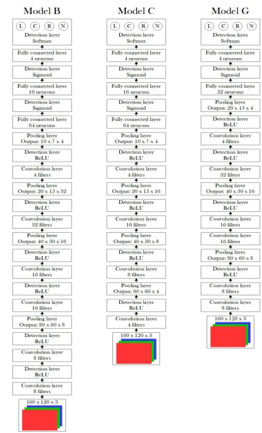
Figure 21 gives a more detailed description of 3 chosen topologies, namely models B, C and G. Note that model G which is the best performer on the training dataset has convolution layers that are immediately followed by an-other convolution layer. That is very benecial for the performance as this model converges much faster that all the other topologies while it reaches a 97% of accuracy which is the highest. The reason may be that by stacking two convolution layers after each other we increase the receptive eld of the second one. That means that we increase the area that a convolutional neuron of the second layer can 'see' through the rst. Doing so in our case, compensates the inability to use larger than3×3kernels. If an activation function is in between

(43)

Finally, gures 22, 23 and 24 depict the feature maps that are being gen-erated after each convolution layer of model C. The choice of model C derives from the fact that it has less convolution layers and the spacial information is better preserved. We show the results of evaluating the CNN with three images which have been generated with our algorithm.

(44)

[image:44.595.135.516.120.748.2]

(45)

[image:45.595.102.468.126.656.2]

(46)

[image:46.595.154.516.127.659.2]

(47)

[image:47.595.104.467.128.661.2]

(48)

3.2.4 Training Dataset Evaluation

The experience of training dierent ConvNets on the generated datasets suggests that they are not suitable for small CNNs and result to bad generalization. Contrary to the large number of false positive predictions that we get if we run the ConvNet on real images, gure 25 shows that this is not the case with the generated ones. We see that for all the models which are depicted in gure 25 the classication error is dominated by misclassication between the positions of the robot. Surprisingly, the existence or not of the robot is predicted almost perfectly even on a newly generated dataset, especially for model G. This leads us to the conclusion that the models overt on the generated dataset.

[image:48.595.198.438.350.612.2]

The later can be conrmed by the observation that the more we train the models, the worse they perform. Any model we train for a lot of epochs will eventually end up unable to detect anything on real images. Even if the robot is in the images the output is stuck into the non-visible (N) class. This indicates that we need a much larger number of dierent poses from the robot or a more sophisticated method to alter the few we already have.

(49)

3.3 Object Localization

Up to this point it has been described how based on the work of Moeys et al. we were able to train relatively small CNNs to perform loose object detection by segmenting the input image into three parts. This method could be sucient to create an end-to-end control like the system in gure 2. After the involvement of Matheus Terrivel[33] in the project though, we redened the specication of the neural network and it was decided to create a more conventional system where the CNN would be part of an object detection pipeline that will localize the GoPiGo robot in greater detail.

In part 3 of the second Chapter, two of the most successful object detectors were briey discussed. They represent two of the main methods that are based on convolutional neural networks for object detection. On one hand, R-CNN is region based and uses a CNN to classify multiple regions of the image. The main drawback of this approach is the number of CNN evaluations that is needed to draw the nal conclusion and this has a serious eect on the computation that is needed and subsequently on the latency of the system. On the other hand, YOLO is much faster and can detect multiple objects with only one evaluation of the CNN. This is possible because the neural network is trained to directly predict the bounding boxes around the objects it detects. A detailed comparison between object detection methods is done in [11].

In our case the most important factors were the time requirements to develop such a system and also its complexity due to the limited resources of the ZYBO board. A sliding-window or region selection based approach like the R-CNN can not be considered due to the aforementioned limitations. Subsequently, the only viable solution was the development of an 'one-shot' detector like YOLO.

In general it is well known that convolutional neural networks have the ability to preserve spatial information throughout the convolution layers [24]. This has been studied, utilized in numerous projects and has led to many state-of-the-art single shot detection algorithms like SSD[19] and Overfeat[30]. The training of those object detection CNNs is not easy though as it requires a training dataset with annotated bounding boxes around the objects to be tracked and expertise on machine learning. In this stage our dataset generation algorithm was proven not very helpful so it was decided to not put more eort and invest time towards altering the generation algorithm to also produce bounding boxes or to develop any new CNN architecture.

Instead we choose a dierent approach after the observation that the last convolutional layer of the ConvNets we trained give enough information to lo-calize the GoPiGo in a very simple way. This is done by summing all the feature maps of the last convolution layer and then just nding the highest value within the 2D matrix which is the result of the summation. This matrix can be inter-preted as a heat map where higher values strongly indicate the presence of the robot.

(50)

The advantage of our method is that we extract the location of the robot with very simple and quick algorithm. Additionally, we avoid any further de-velopment of the CNN or the dataset generation algorithm. We use a simple classier both for detection and localization. The experiments that were per-formed show that this localization technique is robust. Furthermore it can be also used for bounding box prediction if we apply a blob detection algorithm in order to specify the whole region of high activations around it. Instead of only extract the coordinates of the highest value.

Figure 26: The object detection pipeline.

The detection pipeline can be seen in gure 26. First we evaluate the classi-cation CNN on the input image and only if the result is positive we proceed to summing the feature maps and extracting the pixel coordinates of the highest value. A positive result here means when the classier predicts that the robot is in the left (L), central (C) or right (R) part of the image. This information can be used to further reduce the computation by summing and searching only the appropriate part of the image. For example, when the classier indicates that the GoPiGo lays within the left part of image we only need to sum the left half part of the feature maps and then search only there. This results to half the computation compared to the case that we add the feature maps on their full extend.

(51)

[image:51.595.104.440.123.555.2]

(52)

[image:52.595.154.492.123.554.2]