Towards quantification of normal evolution of the human head in order to develop new craniosynostosis measurements

normal evolution of the

human head in order to

develop new

craniosynostosis

measurements

Title Towards quantification of normal evolution of the human head in order to develop new craniosynostosis measure-ments

Author G.A. de Jong

Type Graduate thesis for Technical Medicine

Affiliations Radboudumc

University of Twente

Chairman Prof. dr. ir. C.H. Slump

Medical supervisor Dr. H.H.K. Delye

Technical supervisor UT Dr. ir. F. van der Heijden

Supervisor profession behaviour Drs. P.A. van Katwijk

External member Prof. dr. ir. C.H. Slump

Additional member Dr. T.J.J. Maal

Thesis Format

Some chapters of this thesis are written in article form when applicable. This choice was made since some of the chapters have already been submitted, published as articles or are the basis of a whitepaper for a patent file application. If parts of this article are published or presented it is stated at the beginning of the chapter.

Confidential Sections

Certain sections are marked as confidential as disclosed under NDA A16-0549. These sections were marked as such to allow Radboudumc to file a patent application or (instead of or in addition to filing a patent) to find a commercial partner for exploitation of the technique described in the corresponding section. Please see the non disclosure agreement for further details. The publicly available version of this thesis will only contain the chapter titles.

Digital Media Thesis Guideline

This digital thesis contains 3D models. If you use Adobe Acrobat 9 or higher, or another PDF reader that supports embedded 3D models you can watch this content. In case you have no PDF reader that supports such content you will see a static image. The readability of this document is not compromised by viewing it with the static images alone. The 3D content is solely for an enhanced reader experience.

Figure .0.1:A 3D demo figure of a teapot for testing.

3D . . . Three Dimensional

CCFP . . . Computed Cranial Focal Point

CI . . . Confidence Interval

CPU . . . Central Processing Unit

CT . . . Computed Tomography

CUDA . . . Compute Unified Device Architecture

DC . . . Dual Contouring

GPU . . . Graphics Processing Unit

HU . . . Hounsfield Unit

MC . . . Marching Cubes

MT . . . Marching Tetrahedra

MR(I) . . . Magnetic Resonance (Imaging)

NDA . . . Non-disclosure agreement

Preface ii

Abbreviations iv

1 General Introduction 1

1.1 Thesis outline . . . 2

2 The Computed Cranial Focal Point 7 2.1 Introduction . . . 7

2.2 Materials and Methods . . . 8

2.2.1 Computed Cranial Focal Point Calculation . . . 8

2.2.2 Method Robustness Test . . . 8

2.2.2.1 Shape selection . . . 8

2.2.2.2 CCFP outcome comparison . . . 10

2.2.3 Patient Study . . . 10

2.2.3.1 Patient Study Scan selection . . . 10

2.2.3.2 Segmentation . . . 10

2.2.3.3 Registration . . . 11

2.2.3.4 Patient study outcome comparison . . . 11

2.2.4 Case Studies: Matching of a CT-scan and a 3D photo . . . 11

2.3 Results . . . 12

2.3.1 Method Robustness Test . . . 12

2.3.2 Patient Study . . . 13

2.3.3 Case Studies: Matching of a CT-scan and a 3D photo . . . 14

2.3.3.1 Case 1 . . . 14

2.3.3.2 Case 2 . . . 14

2.4 Discussion . . . 15

2.5 Conclusion . . . 17

2.6 Appendix . . . 18

2.6.2 Calculation Software . . . 18

3 ISO-Surface Extraction for CCFP calculations 21 3.1 Introduction . . . 21

3.2 Criteria of ISO-surface algorithms . . . 21

3.3 History of ISO-surface algorithms . . . 22

3.4 Selection of ISO-surface algorithms . . . 23

3.5 Discussion . . . 24

3.6 Conclusion . . . 25

4 Real-Time Mesh Simplification Using Heterogeneous Computing 29 4.1 Confidential . . . 29

5 Computed Cranial Focal Point in the Adult Population Revised 31 5.1 Introduction . . . 31

5.2 Materials and Methods . . . 31

5.2.1 Segmentation . . . 32

5.2.2 Registration . . . 32

5.2.3 Mesh Simplification . . . 33

5.2.4 Sampling . . . 33

5.2.5 Computed Cranial Focal Point Calculation . . . 34

5.2.6 Hardware and Software . . . 34

5.2.7 Evaluation . . . 34

5.3 Results . . . 34

5.3.1 Segmentation, Registration, Simplification and Sampling . . . 34

5.3.2 Calculated Computed Cranial Focal Point . . . 35

5.3.2.1 Effect of Simplification and Sampling . . . 35

5.4 Discussion . . . 40

5.4.1 CCFP result difference . . . 40

5.4.2 New CCFP Calculation Method . . . 40

5.5 Conclusion . . . 41

5.6 Appendix . . . 41

5.6.1 Improving the CCFP Calculation . . . 41

5.6.1.1 Original CCFP Calculation . . . 41

5.6.1.2 Improved CCFP Calculation . . . 43

6.2 Materials and Methods . . . 46

6.2.1 Patient Study Scan selection . . . 46

6.2.2 Segmentation, Registration, Sampling . . . 47

6.2.3 CCFP Calculation . . . 48

6.2.4 Statistical analysis . . . 48

6.3 Results . . . 48

6.3.1 Trend interpretation . . . 49

6.3.2 Statistical Analysis . . . 50

6.4 Discussion . . . 50

6.5 Conclusion . . . 51

7 Radiation-free 3D head shape and volume evaluation after endoscopically assisted strip craniectomy followed by helmet therapy for trigonocephaly 53 7.1 Introduction . . . 53

7.2 Materials and Methods . . . 54

7.2.1 Orientation and Resampling . . . 55

7.2.2 Volume Analysis . . . 57

7.2.2.1 Statistical Analysis . . . 57

7.2.3 Shape Analysis . . . 57

7.3 Results . . . 58

7.3.1 Volume Analysis . . . 58

7.3.1.1 Comparison of anterior growth percentages . . . 60

7.3.1.2 Statistical Analysis . . . 61

7.3.2 Shape Analysis . . . 62

7.3.2.1 Absolute Shape . . . 62

7.3.2.2 Normalized Shape . . . 64

7.4 Discussion . . . 66

7.5 Conclusion . . . 68

7.6 Appendix . . . 68

7.6.1 Orientation Procedure . . . 68

7.6.1.1 CT-scans . . . 68

7.6.1.2 3D Photos . . . 69

8 General Discussion 73

Craniosynostosis is defined by the premature fusion of cranial sutures with an incidence estimated at 1 in 2000 to 1 in 2500 live births [1]. Classification of isolated craniosynostosis depends on the suture or sutures that are fused [2]. Scaphocephaly occurs with sagittal synostosis and is characterized by long and narrow head growth. Trigonocephaly is caused by the metopic synostosis resulting in a triangular shaped forehead. Plagiocephaly can either occur in anterior form (coronoal synostosis) or anterior form (lambdoid synostosis) with flattening of the affected side of the head. Brachycephaly is a form of craniosynostosis where both of the coronoal sutures are fused resulting in a flat elevated forehead. Oxycephaly occurs when both coronal and sagittal sutures are fused. Craniosynostosis can also occur as a part of a syndrome like Crouzon, Apert, or Pfeiffer [2].

Untreated craniosynostosis can result in increased intracranial pressure as well as impact mental development [2]. There is also an aesthetics aspect to perform an intervention for craniosynostosis. Treatment of craniosynostosis usually occurs by surgery [2, 3]. Each form of craniosynostosis requires different surgical strategies. Multiple strategies can also be present for a single form of craniosynostosis. For instance the open cranial vault reconstruction or (endoscopic) suturectomy with spring- or /helmet therapy for trigonocephaly [4, 5, 6]. The endoscopic suturectomy surgery was introduced as an alternative to the open surgery for sagittal craniosynostosis [7]. In the following years this technique was also adopted for other forms of craniosynostosis, including metopic suture craniosynostosis [8, 9]. However objective monitoring or comparison between techniques is limited.

markers to overlay and match sequential 3D photos for growth monitoring. The current golden standard for overlaying skulls uses the sella turcica, dorsum sella or a nearby structure as skull to skull overlay point due to the assumption that these structures remain immobile during skull growth [19]. However these structures cannot be captured on 3D photos.

The goal of this thesis is to create a method for quantification of the human head evolution based on 3D photogrammetry. Such quantification allows to objectively describe the morphology of the head. Using objective quantification furthermore allows comparison between human heads, or follow-up of the longitudinal evolution of heads. This is of interest after craniosynostosis interventions. Thus the final goal is to use this new method for longitudinal follow-up after craniosynostosis interventions.

1.1.

Thesis outline

Using 3D photos for longitudinal follow-up after craniosynostosis interventions requires a measure for overlaying and matching sequential 3D photos. In the following chapter [Section 2] a new method is proposed using the “Computed Cranial Focal Point” (CCFP) for overlaying CT-scans and 3D Photos with respect to the sella turcica. The robustness of the CCFP is tested in synthetic models. The mean position and standard deviation of the CCFP in the sella turcica-nasion orientation is determined for the adult population. Finally the CCFP is used in the overlaying of a set of 3D photos with CT-scans of children suspected for craniosynostosis.

For the initial CCFP computation certain compensations had to be made. One of the compensations was the volume reduction prior to ISO-surface extraction to reduce computation time. However this technique of volume reduction is slow and also results in loss of details. ISO-surface extraction creates a 3D surface from a set of voxels where the voxel values equal a certain ISO-value. There are many methods for ISO-surface extraction that differ in speed as well as surface properties like the amount of details, amount of faces (triangles) and the occurrence of noise or errors. The CCFP computation becomes slower if an extracted surface has more faces. However less faces can result in an inaccuracy of the surface as well as the CCFP position. Thus an optimum number of faces and details are needed for the CCFP computation. A set of ISO-surface extraction methods are explored in [Section 3]. In addition a scalable mesh simplification technique is introduces in [Section 4]. The combinations of these chapters result in a fast scalable detail preserving ISO-surface extraction and simplification combination that can be used for thus study and CCFP computations in CT-scans.

3D photos that by default have less faces in a mesh compared to surfaces of CT-scans.

With the growth of the human skull it could be possible that the CCFP also shows a change in position relative to the sella turcica over time. In order to quantify this effect a set of CT-scans of pediatric patients are analyzed in [Section 6] similar to that of the adult set from [Section 5]. The CT-scans of these pediatric patients are group by age to determine the change of the CCFP position over time.

Using the CCFP evolution as correction values in 3D photos it is possible to use these photos for longitudinal evaluation of the head shape and volume changes after craniosynostosis interventions. This resulted in the radiation-free 3D head shape and volume evaluation after endoscopically assisted strip craniectomy followed by helmet therapy for trigonocephaly in [Section 7].

Combining these techniques results in a thesis describing the path towards quantification of normal evolution of the human head in order to develop new craniosynostosis measure-ments. Finally this thesis describes a longitudinal follow-up after endoscopically assisted strip craniectomy using the quantification method.

References

[1] Bethany J Slater et al. “Cranial sutures: a brief review.” In:Plastic and reconstructive surgery

121.4 (2008), 170e–8e.issn: 1529-4242.doi: 10.1097/01.prs.0000304441.99483.97.

[2] D. Renier et al. “Management of craniosynostoses”. In:Child’s Nervous System16.10-11 (2000), pp. 645–658.issn: 02567040.doi: 10.1007/s003810000320.

[3] Jayesh Panchal and Venus Uttchin. “Management of craniosynostosis”. In:Plastic and reconstructive surgery111 (2003), 2032–2048; quiz 2049.issn: 0032-1052.doi: 10.1097/01.

PRS.0000056839.94034.47.

[4] Sassan Keshavarzi et al. “Variations of Endoscopic and Open Repair of Metopic Cran-iosynostosis”. In:Journal of Craniofacial Surgery20.5 (2009), pp. 1439–1444.issn: 1049-2275. doi: 10.1097/SCS.0b013e3181af1555.

[5] J. Hinojosa. “Endoscopic-assisted treatment of trigonocephaly”. In:Child’s Nervous System

28.9 (2012), pp. 1381–1387.issn: 02567040.doi: 10.1007/s00381-012-1796-7.

[7] D F Jimenez and C M Barone.Endoscopic craniectomy for early surgical correction of sagittal craniosynostosis.1998.doi: 10.3171/jns.1998.88.1.0077.url: http://www.ncbi.nlm.nih.

gov/pubmed/9420076.

[8] David F Jimenez et al. “Early management of craniosynostosis using endoscopic-assisted strip craniectomies and cranial orthotic molding therapy.” In:Pediatrics110.1 Pt 1 (2002), pp. 97–104.issn: 0031-4005.doi: 10.1542/peds.110.1.97.

[9] C M Barone and D F Jimenez. “Endoscopic craniectomy for early correction of craniosyn-ostosis.” In:Plastic and reconstructive surgery104.7 (1999), 1965–73; discussion 1974–5.issn:

0032-1052.doi: 10.3171/jns.1998.88.1.0077.

[10] JR Marcus, LF Domeshek, and Rajesh Das. “Objective three-dimensional analysis of cranial morphology.” In:Eplasty8 (2007), pp. 175–187.

[11] Jeffrey R Marcus et al. “Use of a three-dimensional, normative database of pediatric craniofacial morphology for modern anthropometric analysis.” In:Plastic and reconstructive surgery124.6 (2009), pp. 2076–84.issn: 1529-4242.doi: 10.1097/PRS.0b013e3181bf7e1b.

[12] Nikoo R Saber et al. “Generation of normative pediatric skull models for use in cranial vault remodeling procedures.” In: Child’s nervous system : ChNS : official journal of the International Society for Pediatric Neurosurgery28.3 (2012), pp. 405–10.issn: 1433-0350.doi:

10.1007/s00381-011-1630-7.

[13] Hans Delye et al. “Creating a normative database of age-specific 3D geometrical data, bone density, and bone thickness of the developing skull: a pilot study”. In:Journal of Neurosurgery: Pediatrics16.6 (2015), pp. 687–702.issn: 1933-0707.doi: 10.3171/2015.4.

PEDS1493.

[14] Jan-Falco Wilbrand et al. “Objectification of cranial vault correction for craniosynostosis by three-dimensional photography.” In: Journal of cranio-maxillo-facial surgery : official publication of the European Association for Cranio-Maxillo-Facial Surgery40.8 (2012), pp. 726– 30.issn: 1878-4119.doi: 10.1016/j.jcms.2012.01.007.

[15] Douglas R McKay et al. “Measuring cranial vault volume with three-dimensional pho-tography: a method of measurement comparable to the gold standard.” In: The Jour-nal of craniofacial surgery 21.5 (2010), pp. 1419–22.issn: 1536-3732. doi: 10.1097/SCS.

0b013e3181ebe92a.

[16] Robert Toma et al. “Quantitative morphometric outcomes following the Melbourne method of total vault remodeling for scaphocephaly.” In:The Journal of craniofacial surgery

[17] P. Meyer-Marcotty et al. “Three-dimensional analysis of cranial growth from 6 to 12 months of age”. In:The European Journal of Orthodontics36.March 2013 (2013), cjt010–.issn:

0141-5387.doi: 10.1093/ejo/cjt010.

[18] Heidrun Schaaf et al. “Three-dimensional photographic analysis of outcome after helmet treatment of a nonsynostotic cranial deformity.” In:The Journal of craniofacial surgery21.6 (2010), pp. 1677–1682.issn: 1049-2275.doi: 10.1097/SCS.0b013e3181f3c630.

This chapter was previously published: [de Jong G a., Maal TJJ & Delye H, The computed cranial focal point. J Cranio-Maxillofacial Surg, 43:1737-1742, 2015. doi: 10.1016/j.jcms.2015.08.023]. There are minor deviations between the this chapter and the publication for a better reading experience for this thesis.

Parts of this chapter were presented or are to be presented at the following events:

• Poster presentation at EANS 2014, Prague (Czech republic), 15th European Congress of Neurosurgery, 12-17 October 2014

• Oral presentation at NVSCA 2014, Rotterdam (Netherlands), 29e najaarsvergadering van de Nederlandse Vereniging voor Schisis en Craniofaciale Afwijkingen, 15 November 2014

• Oral presentation at ECC 2015, Gothenburg (Sweden), 1th European Craniofacial Congress, 24-27 June 2015

• Oral presentation at ESPN 2016, Paris (France), 25th Congress of the European Society for Pediatric Neurosurgery, 8-11 May 2016

• Poster presentation at ISPN 2016, Kobe (Japan), 44th Annual Meeting of the International Society for Pediatric Neurosurgery, 23-27 October 2016

2.1.

Introduction

In the general introduction [Section 1] we introduce one of the main problems of overlaying and matching 3D Photos for growth monitoring without knowledge of the bony structures.

points can be used for sequential photogrammetry matching, by defining the relation between the CCFP -skin and the CCFP-skull and their relative position to the sella turcica.

With the use of the CCFP we aim for a radiation free method to assist in objective sequential measurements of skull growth, to be used in craniosynostosis follow-up. This to reduce the need for CT-scans and thus to reduce the radiation exposure to pediatric patients with craniosynostosis.

2.2.

Materials and Methods

We developed the calculation of the CCFP and tested the robustness of this calculation method. Secondly, we performed an explorative patient study to define the relation between the CCFP-skin and the CCFP-skull and their relative position to the sella turcica. Finally, we used the CCFP-skin to match a CT-scan and 3D photo in two seperate cases to evaluate the potential of the CCFP for matching a CT-scan and 3D photo.

2.2.1. Computed Cranial Focal Point Calculation

The CCFP can be calculated by determining the mean virtual intersection point of all the surface normals. All these intersection points combined create a point cloud in the cranium with a center point and spread (CCFPσ). In depth calculation of the CCFP can be found in Appendix

2.6.

Please see [Section 5.6.1] for the improved CCFP Calculation.

2.2.2. Method Robustness Test

2.2.2.1. Shape selection

The method robustness test was done using a set of predefined shapes as meshes (triangulated objects). Since this is a new method no predefined set of shapes to benchmark the method exists. The shapes were chosen to distinguish the effect on the CCFP and CCFPσ caused by

the conditions that could appear in real world cases. All the shapes are spherically centered around the origin (0,0,0). The x-direction is from medial to lateral as seen from the left side, the y-direction from caudal to cranial and the z-direction from anterior to posterior. We used approximately 50.000 triangles per shape for optimum computation time versus accuracy.

The CCFP and CCFPσof these shapes were calculated and compared with known values

(0, 0, 0) in mm as xyz. The CCFPσis also defined inmmas xyz.

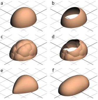
One shape is a sphere with a radius of 9.6cm. There also were 4 hemi-ellipsoid shapes originating from a hemi-ellipsoid with a height and length radius of 9.6cmand a width radius of 7.7cm[Figure 2.2.1(a)]. These measures were chosen to approximate the average human head size. The other 3 hemi-ellipsoid shapes were either asymmetrical cut to remove approximately 20% of the total surface at 15 degrees pitch and 5 degrees roll [Figure 2.2.1(b,d)] and/or irregular deformed up to 2.0cmof the original [Figure 2.2.1(c,d)]. This is to mimic irregular skull shapes and partial missing data as could occur on a CT-scan. There were also two other shapes based on the hemi-ellipsoid resembling respectively trigonocephaly [Figure 1(e)] and scaphocephaly [Figure 2.2.1(f)].

2.2.2.2. CCFP outcome comparison

The sphere, full hemi-ellipsoid and the cut hemi-ellipsoid shapes have a known geometric focal point at the origin. The deformed hemi-ellipsoids shapes and the trigonocephaly- and scaphocephaly- shapes are constructed around the origin but do not necessarily have a geometric focal point at the origin. The position of the CCFP relative to the origin and the CCFPσ to

(0,0,0) for the sphere is caused by polygon inaccuracy and the calculation itself. A similar comparison for the cut and full shapes give the difference caused by removing a part of the shape. Comparing the CCFP and CCFPσbetween the deformed and normal shapes gives the

difference caused by deformation.

The trigonocephaly- and scaphocephaly- shaped hemi-ellipsoid shapes originated from the hemi-ellipsoid with a known focal point at the origin and have been freeform scaled. The difference of the CCFP and the relative CCFP difference compared to the normal hemi-ellipsoid give the error caused by variation.

2.2.3. Patient Study

2.2.3.1. Patient Study Scan selection

For the explorative study, we used scans from patients that underwent a cranial CT-scan in the ER in RadboudUMC between June 2013 and June 2014. Scans showing cranial trauma or structural pathologies were excluded resulting in a group of 36 patients aged 18-65 y.o. (mean 42,6 y.o.) of which 19 were female. The scans were made with a Toshiba Aquilion ONE using a pixel spacing of 0.432mmand a slice thickness of 0.5mmwith a slice resolution of 512x512 by 302 to 376 slices. The scans were anonymized in accordance to local rules from the institutional board of the academic hospital.

2.2.3.2. Segmentation

All the CT-scans were segmented prior to the calculation of the CCFP to obtain the outer surface of the skull and the skin of the head as a mesh. A threshold of -150HUfor the skin and 500

2.2.3.3. Registration

The meshes underwent a translation so that the position of the sella turcica was aligned to the origin (0, 0, 0). Scaling was applied so that 1 unit in the mesh-space equals 1 mm.

The meshes were aligned with the sella nasion plane crossed with the horizon of the sphenoid at the sella turcica as the horizontal plane. Axis were directed so that sella to cranial is the positive y-direction, the sella to posterior is the positive z-direction, and the right to left is the positive x-direction. All triangles of the mesh y < -5mm of the sella turcica were omitted in further calculations.

2.2.3.4. Patient study outcome comparison

The main goal of the patient study is to investigate the relation between the CCFP-skull and CCFP-skin. The secondary goal is to determine the relation between the CCFP-skull/CCFP-skin and the sella turcica.

2.2.4. Case Studies: Matching of a CT-scan and a 3D photo

The first case was a 9 month old female suspected of craniosynostosis of which a 3D photo was made. A CT-scan followed 3 weeks after the photo disproving craniosynostosis. The second case was a 3 month old female patient with suspected craniosynostosis of which a CT-scan was made proving trigonocephaly. For further evaluation a 3D photo of this patient was made 6 weeks after the CT-scan. Both cases were individually used for matching the CT-scan and 3D photo using the CCFP.

In prospect to the results of the patient study we can say that the relative position between sella turcica, CCFP-skin and CCFP-skull is predictable. Due to this property of the CCFP values we can use the CCFP for matching. Hence the CCFP-skin of a 3D photo and CT-scan was used. Per case the CCFP-skin was calculated for both the CT-scan and 3D photo. We aligned and rotated the CT-scan similar to that of the patient study. We transformed the 3D photo with the CCFP-skin to the CCFP-skin of the CT-scan. The 3D photo was then manually rotated to match the CT-scan using the CCFP as a pivot.

2.3.

Results

2.3.1. Method Robustness Test

The method robustness test focused on the accuracy of the CCFP for a known focal point and the spread of the CCFPσfor various meshes. All given CCFP coordinates and CCFPσstandard

deviations are presented in [Table 2.3.1].

Table 2.3.1:The distance in for X, Y, Z from 0,0,0 to the CCFP and the standard deviation of X,Y,Z for the test models in mm.

CCFP(mm) CCFPσ(mm)

Structure X Y Z σ(X) σ(Y) σ(Z)

Sphere 0.0 0.0 0.0 0.01 0.01 0.01

Hemi-ellipsoid 0.0 7.7 0.0 8.3 2.7 5.6 Hemi-ellipsoid cut 0.8 7.0 1.1 9.2 2.5 6.0 Hemi-ellipsoid deformed -0.7 9.8 0.8 9.9 8.4 9.9 Hemi-ellipsoid deformed and cut -1.6 10.0 0.9 9.6 7.8 11.7 Hemi-ellipsoid trigonocephaly 0.0 -5.6 10.7 9.5 5.7 9.7 Hemi-ellipsoid scaphocephaly 0.0 -6.2 -0.1 12.1 24.5 7.2

In the sphere there was no measurable deviation for the CCFP and a (0.01, 0.01, 0.01)

mmspread for the CCFPσ. This can be considered negligible in CT-scans with a voxel spacing

size of 0.5mm3_.

The full, cut, and deformed hemi-ellipsoid shapes have a predominant y-component for the CCFP around 8mmand small x- and z-components (ranging from -0.7 to 1.1mm). Do note that the CCFP does not have to represent the geometrical focus. The distance between the full and the cut hemi-ellipsoid is 1.5mmand between the full and deformed hemi-ellipsoid is 2.4mm. The distance between the deformed ellipsoid and the deformed and cut hemi-ellipsoid is 0.9mm. Removing approximately 20% of the surface results in a smaller difference of the CCFP than applying up to 2cmdeformations to the surface. In case of deformations the difference caused by the cut is almost similar to the cut alone.

The trigonocephaly hemi-ellipsoid has a CCFP of (0.0, -5.6, 10.7). This deviates 17.1mm

from the full hemi-ellipsoid and is most present in the y- and z-direction. The scaphocephaly hemi-ellipsoid in contrast has a CCFP of (0.0, -6.2, -0.1) which only significantly deviates in the y-direction from the full hemi-ellipsoid (13.9mm).

The spread for the tirgonocephaly primarily deviates from the full hemi-ellipsoid in the y- and z-direction. The spread for the scaphocephaly deviates in all directions with the highest deviation in the z-direction up to 24.5mm.

2.3.2. Patient Study

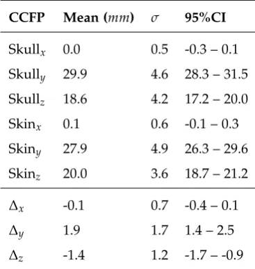
The results of the CT-scans can be found in [Table 2]. The CCFP (mm) is expressed as relative to the sella turcica (0, 0, 0) in the sella-nasion orientation. The average CCFP-skull is at (-0.4, 28.9, 18.0) with aσ(0.5, 4.5, 4.4) while the CCFP-skin is at (0.0, 27.1, 19.4) with aσ(0.6, 4.6, 3.9).

Using a Shapiro-Wilk test resulted in proven normal distributions in the x- and y-direction with CCFP-skull p-values of (0.226, 0.452, 0.000) and CCFP-skin p-values of (0.388, 0.526, 0.001).

The difference between theσof the CCFPs is in sub-millimeter scale. The mean CCFP

differs (-0.1, 1.9, -1.4) from skull to skin with a maximumσof 1.4mmand a maximum 95% CI

of mean±0.6mm.

Table 2.3.2:The mean CCFP, standard deviation and 95% CI for the population of 36 patients for the skull, skin and difference between the skull and skin (∆) in mm.

CCFP Mean (mm) σ 95%CI

Skullx 0.0 0.5 -0.3 – 0.1

Skully 29.9 4.6 28.3 – 31.5

Skullz 18.6 4.2 17.2 – 20.0

Skinx 0.1 0.6 -0.1 – 0.3

Skiny 27.9 4.9 26.3 – 29.6

Skinz 20.0 3.6 18.7 – 21.2 ∆x -0.1 0.7 -0.4 – 0.1

∆y 1.9 1.7 1.4 – 2.5

2.3.3. Case Studies: Matching of a CT-scan and a 3D photo

2.3.3.1. Case 1

Visual representation of the registration in 3D shows a nicely matched overlay [Figure 2.3.1]. The colors represent the difference between the 3D photo and CT-scan. The overlay shows the origin at the sella turcica as obtained from the CT-scan. A blue circle at the top shows the position of the maximum difference as caused by the hairnet.

The absolute average raycast difference was 0.7mmwith a standard deviation of 1.1mm. The biggest difference was 6.72mmat the bulge of the hairnet but did not seem to significantly impact the average.

Figure 2.3.1:Overlaying and distance map of a 3D photo and CT-scan using CCFP-skin matching and manual rotation in a 9 month old female patient.

2.3.3.2. Case 2

the position of the maximum difference as caused by the hairnet. Again the colors represent the difference between the 3D photo and CT-scan.

The absolute average raycast difference was 2.3mmwith a standard deviation of 1.1mm. The biggest difference was 6.44mmat the bulge of the hairnet at the back of the head.

Figure 2.3.2:Overlaying and distance map of a 3D photo and CT-scan using CCFP-skin matching and manual rotation in a 3 month old female patient.

2.4.

Discussion

The segmentation process was done in Matlab [20] resulting in some limitations. Es-pecially when CT scan was performed with considerable head flexion, segmentation and registration resulted in a smaller usable section for CCFP calculation. Missing data did not influence the CCFP calculation significantly in the robustness test, however accuracy improves utilizing all data. Changing the segmentation process in Matlab could resolve this issue. Another option is using software like ITK-snap to handle the segmentation [23].

The patient study consisted of 36 patients and was of an explorative nature. Hence the study only gives an indication of the distribution of the CCFP among the adult population. Using a larger sample results in even more accuracy, although this study showed a small 95% CI spread for CCFPs. Yet the few millimeter 95% CI spread for CCFPs suggest that the mean position for the CCFPs between individuals is at about the same position relative to the sella turcica. The 95% CI sub-millimeter spread for the mean difference between the CCFP-skin and CCFP-skull suggests that the position relative to each other is predictable.

The case studies of matching 3D photos with CT-scans using the CCFP showed a very high agreement. A follow-up study is needed to show pitfalls or problems during this process. Although the absolute average difference is bigger than in first case, the standard deviation of the difference is almost equal in both cases. This can be explained by the time between the CT-scan and 3D photo as well as the order in which these were taken. In the first case the 3D photo was made prior to the CT-scan which added the hairnet to the overall 3D photo volume but where growth added to the CT-scan volume and thus somewhat compensating each other’s additional volume. In the second case the CT-scan came prior to the 3D photo which allowed both the hairnet and the additional growth time (3 versus 6 weeks) to add to the volume of the 3D photo. Therefor it is to be expected that there was a bigger absolute average difference compared to the first case. Taking this in consideration as well as the near equal standard deviation and the visual inspection suggests that in both cases the overlay was performed with equal accuracy. Finally the trigonocephaly did not seem to impact the matching process. Further differences could be caused by inaccuracy of the 3D-photo system or the CT-scan and its segmentation or registration.

In a growing skull, the CCFP could change and might require parametric correction to be able to perform sequential overlay of 3D photo data. This should be the subject of a follow-up study with CT-scans in different pediatric age groups. The CCFPσwas only used

for the method robustness test and was not further evaluated in the patient study. The CCFPσ

might give insight in the shape of the head as well as the effect of possible abnormalities of the head as suggested in the robustness test for the trigonocephaly and scaphocephaly shapes. This should be looked into and can potentially be used in clinical practice.

process. This could result in small variation differences from patient to patient. An automated method to determine the rotations in these parts would be more objective and thus less vulnerable to these errors.

2.5.

Conclusion

We have shown that the calculation of the CCFP is reliable and robust against deformations and missing data. Furthermore there is a considerable relative difference for the CCFP position in the synthetic shapes of the simulated trigonocephaly and scaphocephaly compared to the other shapes. This relative difference could potentially be used to quantify and/or qualify these conditions in CT-scans or 3D photos. Future research should be directed to investigate these features.

In the adult population, the CCFP-Skin and CCFP-Skull only differ a few millimeter in mean, 95% CI and standard deviation. Thus obtaining either of these values can be used to accurately estimate the other value. Since the difference of the CCFP-skin and CCFP-skull show few millimeter variations in individuals, the CCFP-skin can be used as an indication to where the sella turcica is located.

The CCFP-skull lies at average 1.9mmmore cranial and 1.4mmmore anterior than the CCFP-skin. The CCFP-skin is at (0.0, 27.1, 19.4)mmand the CCFP-skull at (-0.1, 28.9, 18.0)mm

with a few-millimeter 95% CI, in relation to the sella turcica.

We have shown that the alignment of the skin surface of a 3D photo to a CT-scan while using the CCFP translation and manual rotation results in a near perfect match. We have shown a fit with an average sub millimeter difference in the first case and 2.3 mm difference in the second case which can be explained by growth and the use of a hairnet. In both cases there was a very small standard deviation for the difference (1.1 mm) suggesting that both cases were matched with equal accuracy. The hairnet in the 3D photo, and the missing data in the CT-scan had no observable impact on the CCFP calculation and matching. Hence the CCFP matching method is a viable option to match 3D photos with CT-scans. This could be done with sequential 3D photos as well, reducing the need for CT-scans and the radiation dose in the follow-up of cranial development.

and in relation to other cranial measurement methods. Distinguishing between age and sex can give insight in the CCFP in the developing cranium. But most important is the potential to reduce the need for CT-scans, along with the radiation exposure in the follow-up of cranial development by using the CCFP.

2.6.

Appendix

2.6.1. CCFP Calculation

The CCFP is calculated by determining the average of so called center points in a triangulated spherical object. Each face/triangle/polygon in the triangulated object has a center and a normal. Each center and normal can be considered as a skew line with the origin in the face center and the direction as the face normal. A so called center point can be calculated for each combination of skew lines that can be made. A center point is a point between two skew lines that has the closest and equal distance to two skew lines. For this the positions s and t on lines

Ln(s)andLm(t)are used to calculate the center point as shown in Ericson, Real-Time Collision

Detection, 2005, (Chapter 5.1.8) [24]. An example of two skew lines and their center point is given in [Figure 2.6.1].

Averaging all skew line combinations for one given face gives the center-point (Pc,Ln) for

that face as can be seen in [Equation 2.6.1]. Only skew line combinations that have an absolute angle between each other larger than 30 degrees (and smaller than 330 degrees) will be used in the calculation. These cases will be add to the count of nf,Ln as well. This is to exclude

near-parrallel face calculations that would result in outliers.

Pc,Ln =

1

nf,Ln

∑

Ln(s) +Lm(t)

2 (2.6.1)

Finally all center points are averaged to get the CCFP as can be seen in [Equation 2.6.2].

CCFP= 1 nf aces

nf aces

∑

n=1

Pc,Ln (2.6.2)

2.6.2. Calculation Software

−10 −5

0 5

10

−10 −5 0 5 10 −10 −5 0 5 10

Figure 2.6.1:Example of two skew lines and the center point in 3D. A green line is drawn between two non-intersecting skew lines (red and blue) where the distance between these skew lines is shortest. The center of this green line is a center point. The distance from the center point to the each skew lines is equal.

the standard deviation and average of these center points. The software used was as proof of concept and thus the CCFP calculation is not limited to Matlab or C++. Other software (e.g. the free alternative Octave [25]) could be used to implement the CCFP calculation. Other acceleration techniques like CUDA [26] instead of OpenCL could also be used. Due to the simple math in the CCFP calculation completely stand-alone software could be written if desired.

References

[20] The MathWorks Inc. “MATLAB and Statistics Toolbox Release 2014a”. In:Natick, Mas-sachusetts, United States(2014).

[21] Tomas Möller and Ben Trumbore. “Fast, minimum storage ray/triangle intersection”. In:

[22] JE Stone, David Gohara, and Guochun Shi. “OpenCL: A parallel programming standard for heterogeneous computing systems”. In:Computing in science & engineering(2010).doi:

10.1109/MCSE.2010.69.

[23] L Ibanez et al.The ITK Software Guide. Vol. Second. May. Kitware, Inc., 2005, p. 804.isbn:

1930934157.

[24] Christer Ericson. “Chapter 5 - Basic Primitive Tests”. In:Real-Time Collision Detection. Ed. by Christer Ericson. The Morgan Kaufmann Series in Interactive 3D Technology. San Francisco: Morgan Kaufmann, 2005, pp. 125–233.isbn: 978-1-55860-732-3.doi: 10.1016/

B978-1-55860-732-3.50010-3.

[25] John W. Eaton.GNU Octave.url: http://www.gnu.org/software/octave/ (visited on

08/19/2015).

culations

3.1.

Introduction

CT-scans and other volume based imaging modalities use a set of voxels (3D pixel) to describe a volume. Certain computations executed on CT-scans are only possible or greatly benefit from vectorized surface data rather than voxel based data.

There are several methods of obtaining vectorized surface information from voxels; a process called (ISO-)surface extraction. ISO-surface extraction extracts a surface from a set of voxels where the voxel value equals a certain ISO-value. However there are differences between the ISO-surface extraction methods. This can for instance be the amount of details, the overall number of faces, the occurrence and amount of artifacts, the computation time.

The Computed Cranial Focal Point (CCFP) is a point in the cranium with a fixed position relative to the sella turcica that can be calculated based on such vectorized data [27]. This point can be calculated by using 3D models obtained from CT-scans or 3D Photos. The CCFP calculation uses surface normals and surface normal origins to determine the CCFP and its point-cloud.

The goal of this chapter is to perform a literature study to determine what the best ISO-surface algorithm is for the use in a CCFP computation pipeline. We look at the differences in the ISO-surface extraction methods regarding the numbers of faces, details, and artifacts of the mesh as well as the algorithms’ computation times.

3.2.

Criteria of ISO-surface algorithms

consideration is speed. With the current processing power there should be no need for long processing times. The amount of generated triangles was also of importance. More triangles describing the same surface usually accounts for more processing time in later steps. Another aspect to look at was the presence of artifacts and in what form they occurred.

Finally we looked if there were readily available implementations of the algorithm that could be integrated in Matlab 2015a (8.5) [28] with or without the use of C++.

3.3.

History of ISO-surface algorithms

The oldest forms of (ISO-)surface extraction methods either focused on specific structures [29] or had know artifacts in the contour line implementation [30, 31].

A newer form of ISO surface extraction was the so called “Marching Cubes” (MC) algorithm (patented 1985-2005) [32]. MC uses look-up tables to define the set of triangles to be used as a replacement of a voxel. This was done by checking the ISO-values of neighboring voxels to choose an appropriate set of triangles from the look-up table. The use of look-up tables inspired another ISO-surface algorithm: “Marching Tetrahedra”[33] (MT). MT was a patent free alternative to MC with a different look-up table, triangle set and look-up method. Several suggested improvements on these algorithms have been made tackling specific per solution issues [34, 35, 36, 37, 38, 39].

A known property of the look-up table based algorithms was the inability to vary triangle size other than defined in the look-up table. This means that every triangle created would fit inside a voxel. As a result large flat surfaces that could easily described with a few triangles are still described with at least as many triangles as there are voxels multiplied by the result of the look-up table. A single flat surface inside a voxel can hold up to 6 triangles in MC. A combination of both these properties can result in a very large amount of triangles for a single ISO-surface [40, 37, 41, 42].

In 1998 the surface nets method was introduced [43]. This is an iterative method that smooths out a cubic mesh based on the ISO-values to an optimum value for surface approximation. The issue with surface nets is that it is unable to produce sharp contours. A similar method called dual contouring was introduced to enable sharp corners [44]. As an addition it also includes a level of detail implementation based on octree simplification guided by quadric error functions.

reduce the triangle count as well [42]. Another early example utilizes merging and patching based on marching cubes and octree data [41]. Other forms combining MC with octree data are also known [45].

One of the latest known generations of ISO-surface algorithms are based on (surface) distribution algorithms of points or rays. The use of these algorithms require other techniques to acquire the point clouds. These can for instance be based on voronoi diagrams [46], on partial differential equations [47], or on least-squares projection [48]. Using the ISO-surface point cloud determination on a volume allows the use of techniques like interpolation, splines and quadrics to determine a more accurate and smooth point cloud. However these latest generations are more commonly used with point clouds acquired from laser scanners, IR based 3D cameras or similar rather than on volume datasets.

3.4.

Selection of ISO-surface algorithms

The oldest techniques from the inventory are unsuitable due to not being suitable for true ISO-surface extraction.

The latest known generations are also unsuitable due to the use of additional point cloud generation techniques contributing in a large degree to the extraction time. For instance the least-squares projection technique takes from 21.3 to 36.8 seconds for a 75 thousand points point cloud in 2010 excluding the actual ISO-surface extraction itself [48]. Comparing this to a graphics processing unit (GPU) implementation using CUDA[26] MC algorithm of a magnetic resonance (MR) Brain results in processing from 10 to 305 million voxels per second in 2008 [49]. Although voxels and points in a point cloud are different objects in processing, comparing these speeds gives an idea of the difference in performance while trying to achieve a similar result; ISO-surface extraction.

So in essence the techniques to be further investigated are based on look-up tables (marching cubes or marching tetrahedra) and on interpolating methods (surface nets and dual contouring). All of these techniques so far have native or later implemented GPU implementations [49, 50, 51, 44, 52, 53] which is a good indication of fast processing.

MT is known to have an approximately four times higher triangle count compared to MC. Variations to reduce the amount of triangles using MT have been made [37]. However the GPU implementation is based on the original MT method [53]. Due to the high amount of triangles created (16 million is easily possible in a skull-ct) MT is no feasible option for now.

DC and surface nets have much in common. However dual contouring is able to represent sharp edges [54, 44, 51]. With the optional level of detail feature this is an interesting algorithm.

So in essence we have come to MC and DC as the final options. In the basic form both MC and DC have issues with non-manifold regions if two non-connected voxels are near. For both of these algorithms solutions have been proposed to fix these non-manifold regions [34, 54]. Furthermore in general DC produces less or an equal amount triangles than MC at the highest level of detail. Unfortunately the GPU implementations of both MC and DC do not have the non-manifold region fixes.

There is a small difference in quality for the GPU implementations of MC and DC. DC generally produces better quality meshes regarding the radii-ratio [51, 55].

Thus in the preference for the ISO-surface algorithm would be DC. Unfortunately there is no public GPU implementation of DC. Implementing the algorithm on the GPU from scratch was not a part of the scope of this study.

So in the end we will fall back on the OpenCL implementation of Marching Cubes as a second best. The algorithm, source code, and article [50] on this implementation are publicly available and thus our preferred choice.

3.5.

Discussion

OpenCL Accelerated MC was our second best choice for ISO-surface extraction. DC is a promising measure with a higher quality however not readily available for implementation in Matlab 2015a. In future work we will look at the possibility for implementing DC in Matlab.

To date new ISO-surface algorithms are developed and older algorithms are updated to specifically target issues for certain applications. One of the main issues is the great number of available ISO-surface algorithms and the lack of systematic reviewing. Most articles will focus on just reviewing a single algorithm and comparing that towards other algorithms that they consider either standard, new, or otherwise relevant [35, 56, 51, 57]. This makes it difficult to properly select the ISO-surface algorithm that is best suited for a study or project.

study or project.

3.6.

Conclusion

We reviewed a set of ISO-surface extraction algorithms to use on medical volume data. We looked into execution time, amount of generated triangles, accuracy, occurrence of artifacts and the availability of the algorithm for implementation in Matlab.

Our initial pick was Dual Countours based on the execution time, amount of triangles, and the accuracy. However there was no implementation with public source code available to implement in Matlab. Hence we choose for OpenCL accelerated Marching Cubes. With somewhat lesser accuracy and more triangles compared to DC this was our second choice based on the figures. However due to the availability we finally picked MC.

There are a large amount of other ISO-surface algorithms and the lack of standardized testing and evaluation made this review cumbersome to say the least. We reviewed the most common ISO-surface algorithms available. Many “exotic” ISO-surface algorithms were not reviewed for this study. We would like to suggest that ISO-surface algorithms in the future to be all tested in a similar fashion covering the most important aspects like computation time, triangle count, accuracy, artifacts, etc. This should greatly help to choose the ISO-surface algorithm best suited for a study or project in the future.

Furthermore we will look into dual contouring on the GPU in a generalized form for implementation in Matlab or similar software in future studies.

References

[26] John Nickolls et al. “Scalable parallel programming with CUDA”. In:Queue6.2 (2008), p. 40.issn: 15427730.doi: 10.1145/1365490.1365500.

[27] G. A. De Jong, T. J J Maal, and H. Delye. “The computed cranial focal point”. In:Journal of Cranio-Maxillofacial Surgery43.9 (2015), pp. 1737–1742.issn: 18784119.doi: 10.1016/j.jcms.

2015.08.023.

[28] United States Natick, Massachusetts.Matlab 2015a. Massachusetts, United States, 2015. [29] Christian Barillot et al. “3D Reconstruction of Cerebral Blood Vessels”. In:IEEE Computer

Graphics and Applications5.12 (1985), pp. 13–19.issn: 0272-1716.doi: 10.1109/MCG.1985.

276258.

[31] Larry Cook et al. “A Three-Dimensional Display System for Diagnostic Imaging Applica-tions”. In:IEEE Computer Graphics and Applications3.5 (1983), pp. 13–19.issn: 0272-1716. doi: 10.1109/MCG.1983.263180.

[32] William E. Lorensen and Harvey E. Cline. “Marching cubes: A high resolution 3D surface construction algorithm”. In:ACM SIGGRAPH Computer Graphics21.4 (1987), pp. 163–169.

issn: 00978930.doi: 10.1145/37402.37422.

[33] Jules Bloomenthal. “Polygonization of implicit surfaces”. In:Computer Aided Geometric Design5.4 (1988), pp. 341–355.issn: 01678396.doi: 10.1016/0167-8396(88)90013-1.

[34] Sundaresan Raman and Rephael Wenger. “Quality Isosurface Mesh Generation Using an Extended Marching Cubes Lookup Table”. In: 27.3 (2008), pp. 3–10.

[35] Paul Ning and Jules Bloomenthal. “Evaluation of implicit surface tilers”. In:IEEE Computer Graphics and Applications13.6 (1993), pp. 33–39.issn: 02721716.doi: 10.1109/38.252552.

[36] Samir Akkouche and Eric Galin. “Adaptive implicit surface polygonization using march-ing triangles”. In:Computer Graphics Forum20.2 (2001), pp. 67–80.issn: 01677055.doi:

10.1111/1467-8659.00479.

[37] G M Treece, R W Prager, and A H Gee.Regularised marching tetrahedra: improving iso-surface extraction. Tech. rep. CUED/F-INFENG/TR 333. 1998.doi: http://dx.doi.org/10.1016/

S0097-8493(99)00076-X.

[38] Leif Kobbelt et al. “Feature Sensitive Surface Extraction from Volume Data”. In:Siggraph

D (2001), Pages: 57–66.doi: 10.1145/383259.383265.

[39] S.L. Chan and E.O. Purisima. “A new tetrahedral tesselation scheme for isosurface generation”. In:Computers & Graphics22.1 (1998), pp. 83–90.issn: 00978493.doi: 10.1016/

S0097-8493(97)00085-X.

[40] Heinrich Müller and Michael Stark. “Adaptive generation of surfaces in volume data”. In:

The Visual Computer9.4 (1993), pp. 182–199.issn: 01782789.doi: 10.1007/BF01901723.

[41] R. Shekhar et al. “Octree-based decimation of marching cubes surfaces”. In:Proceedings of Seventh Annual IEEE Visualization ’96(1996).doi: 10.1109/VISUAL.1996.568127.

[42] C. Montani, R. Scateni, and R. Scopigno. “Discretized Marching Cubes”. In:Proceedings Visualization ’94(1994).issn: 10702385.doi: 10.1109/VISUAL.1994.346308.

[43] Sff Gibson. “Constrained elastic surface nets: Generating smooth surfaces from binary segmented data”. In:Medical Image Computing and Computer-Assisted Interventationâ ˘A ˇ TMIC-CAI’98(1998), pp. 888–898.issn: 16113349.doi: 10.1007/BFb0056277.

[45] Scott Schaefer and Joe Warren. “Dual marching cubes: Primal contouring of dual grids”. In:Computer Graphics Forum24.2 (2005), pp. 195–201.issn: 01677055.doi:

10.1111/j.1467-8659.2005.00843.x.

[46] M. Alliez, P. and Cohen-Steiner, D. and Tong, Y. and Desbrun. “Voronoi-based variational reconstruction of unoriented point sets”. In:Proceedings of the fifth Eurographics symposium on Geometry processing(2007), pp. 39 –48.issn: 17278384.doi: 10.1145/1281991.1281997.

[47] Paul Rosenthal and Lars Linsen. “Smooth surface extraction from unstructured point-based volume data using PDEs”. In: IEEE Transactions on Visualization and Computer Graphics14.6 (2008), pp. 1531–1538.issn: 10772626.doi: 10.1109/TVCG.2008.164.

[48] Dong Jin Yoo. “Rapid surface reconstruction from a point cloud using the least-squares projection”. In:International Journal of Precision Engineering and Manufacturing11.2 (2010), pp. 273–283.issn: 12298557.doi: 10.1007/s12541-010-0031-2.

[49] Christopher Dyken et al. “High-speed marching cubes using histopyramids”. In:Computer Graphics Forum27.8 (2008), pp. 2028–2039.issn: 01677055.doi: 10.1111/j.1467-8659.2008.

01182.x.

[50] Erik Smistad, Anne C. Elster, and Frank Lindseth. “Real-Time Surface Extraction and Visualization of Medical Images using OpenCL and GPUs”. In:Nik-2012november (2012), pp. 141–152.

[51] L. Schmitz et al. “Efficient and quality contouring algorithms on the GPU”. In:Computer Graphics Forum29.8 (2010), pp. 2569–2578.issn: 01677055.doi: 10.1111/j.1467-8659.2010.

01825.x.

[52] ARM Limited.Procedural modelling with geometry shaders.url: https://malideveloper.arm.

com/resources/sample-code/procedural-modelling-with-geometry-shaders/.

[53] Miłosz Ciznicki et al. “Efficient isosurface extraction using marching tetrahedra and histogram pyramids on multiple GPUs”. In:Lecture Notes in Computer Science (including subseries Lecture Notes in Artificial Intelligence and Lecture Notes in Bioinformatics) 7204 LNCS.PART 2 (2012), pp. 343–352.issn: 03029743.doi: 10.1007/978-3-642-31500-8_35.

[54] Scott Schaefer, Tao Ju, and Joe Warren. “Manifold Dual Contouring”. In: (), pp. 1–10. [55] C. A. Dietrich et al. “Edge transformations for improving mesh quality of marching

cubes”. In:IEEE Transactions on Visualization and Computer Graphics15.1 (2009), pp. 150– 159.issn: 10772626.doi: 10.1109/TVCG.2008.60.

[57] Timothy S. Newman and Hong Yi. “A survey of the marching cubes algorithm”. In:

Computers and Graphics (Pergamon)30.5 (2006), pp. 854–879.issn: 00978493.doi: 10.1016/j.

Heterogeneous Computing

4.1.

Confidential

The current chapter "Real-Time Mesh Simplification Using Heterogeneous Computing" is confidential, disclosed under NDA A16-0549.

Adult Population Revised

5.1.

Introduction

The Computed Cranial Focal Point (CCFP) was introduced byDe Jong et al. (2015)as a tool to assist head comparison based on soft-tissue from 3D Photos or CT-scans [27]. This method was improved by accounting for triangle size differences as could occur in 3D Photos or surfaces of CT-scans [Chapter 5.6.1]. Additional suggestions were made in the original article to further improve the calculation in the segmentation and registration process.

We aim for the best possible results and continuous improvement of the CCFP computa-tion making it available for public use. Since we are aware that there were uncertainties in the original computation pipeline we decided to revise the original CCFP calculation pipeline.

Our goal of this chapter is to revise and optimize the original CCFP calculation pipeline for CT-scans. We look in depth in improving the segmentation, registration and simplification process. For longitudinal and grouped comparison we introduce sampling. We will test several levels of sampling where we will look at execution time, duplicate face samples and the CCFP positions relative to the sella turcica.

5.2.

Materials and Methods

Segment ation Registration Simpl ification

Sampl ing

CCFP Calc .

Start

OpenCL 16 to 8 bit clamping around ISO-value OpenCL 8-bit Marching Cubes Small Object Removal

Align Nasion on y-axis

Align clenoid processes perpendicular to

y-axis Sella Turcica at

(0,0,0) OpenCL Mesh Simplification OpenCL Icosphere Raycasting from Sella turcica Improved CCFP Calculation End Gap filling

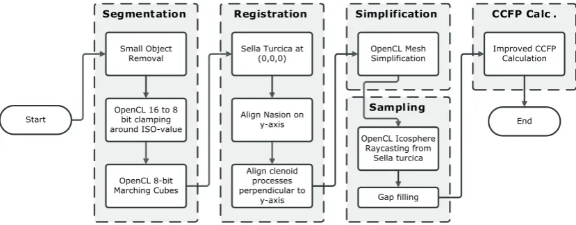
Figure 5.2.1:The revised CCFP calculation pipeline for CT-scans

5.2.1. Segmentation

We started with small object removal for objects with a Hounsfield unit (HU) of 167 and above. Objects not connected with a 18-connected neighborhood to the biggest object (skull) with a HU of 167 and above were removed. Segmentation was performed by a modified version of the OpenCL Marching Cubes (MC) implementation bySmistad et al. (2012)at an ISO-value of 167 HU[50]. The original implementation only accepted 8-bit volume data due to memory limitations while nearly all modern CT volume data uses 16-bit values storing the HU as signed 16-bit integers. Converting the volume by directly applying the threshold to have a binary image could result in jagged edges on the reconstruction. In order to overcome this issue we clamped the CT-scan in the range of -128 to 127 (signed 8 bit limit) with the threshold at 0 [Equation 5.2.1]. We subtracted the original threshold value and added 127 to every voxel value while clamping values <-128 to -128 and >127 to 127. This allowed 8-bit signed storage of the CT-scan in the range of the threshold. This is a lossless conversion regarding output mesh quality when compared to true 16-bit MC. Applying the MC algorithm on this new 8-bit dataset at an ISO-value of 0 resulted in a mesh with several millions of faces.

HU8bit,clamp=clamp(HU16bit−iso,−128, 127) (5.2.1)

5.2.2. Registration

the y-axis with the top of the skull in the z-direction. The clinoid processes are used to rotate the skull around the sella-nasion axis to place the midsaggital plane of the skull in the y-z plane. Manual rotational correction was applied if necessary due to the error in rotation caused by the natural variation in the clinoid processes [59, 60].

5.2.3. Mesh Simplification

Since a mesh with several million faces is impractical for the calculation time mesh simplification is an option. Furthermore in [Section 2] it is stated that we would require approximately 50.000 triangles for optimum computation time versus accuracy [27]. However this was based on some of the limitations that were in the original [Section 2]. Thus we used two levels of mesh simplification to reduce the number of triangles while maintaining the shape of the skull [See Section 4]. In this step we reduce the amount of triangles with 128-grid and 256-grid simplification. As a reference we also use no simplification at the cost of computation time.

5.2.4. Sampling

In order to further reduce the amount of triangles and explore a new optimum amount of triangles for computation we use sampling with an OpenCL implementation of raycasting [21]. Sampling is the technique of picking a (sub)set of datapoints from another set of datapoints or to approximate the original object. Since the original mesh is already sampled due to the simplification process we perform resampling to further reduce the number of data points. In our case the process of resampling allows to describe the surface as a set of datapoints of a reference shape. Raycasting is the technique of retrieving a data point from an intersection of a ray and a (triangulated) surface.

The resampling is done using raycasting [21] and a generated hemi-icosphere (half icosphere) as reference shape [61]. Each ray for sampling starts at the origin and crosses a vertex from the icosphere from where it can intersect with the registered and simplified CT-scan. Ray lengths of the intersection are stored and used to determine a new vertex point for resampling. We sample with different hemi-ico spheres with different numbers of vertices. We start at 91 samples up to 82241 samples.

A single triangle can be sampled multiple times by different rays depending on the size and position of the triangle as well as the direction and amount of rays. The amount of double samples indicate the usefulness of the sampling. In general the usefulnesses of the sampling deceases if the amount of double samples increase.

by ring loop over 50 iterations to fill the small gaps. This was also execution with the aid of OpenCL.

5.2.5. Computed Cranial Focal Point Calculation

Although the mesh achieved from the sampling has relatively small deviations in face size compared to 3D Photos we still used the improved CCFP Calculation [Section 5.6.1]. This improved calculation compensates for face size differences that can occur in meshes. Using this method gives us the CCFP location per skull expressed as the relative position inmmas oriented in the sella-nasion orientation with midsaggital symmetry.

5.2.6. Hardware and Software

All calculations were performed using Matlab 2015a (8.5) [28] with C++ and OpenCL 1.2 [22]. OpenCL and C++ were used for the 16 to 8 bit clamping, the MC, mesh simplification, sampling and CCFP calculation.

All computations were executed on a Xeon E5 1620 v3 (3.5 Ghz) with 32 Gb RAM. As an OpenCL accelerator we used a GeForce GTX 970 with 4 Gb RAM.

5.2.7. Evaluation

For evaluation we compare the new CCFP value with the earlier reported CCFP value as found in the original study [27]. We further look into effect of the number of raycast samples on the mean CCFP, theσof the CCFP, 95% CI, the amount of doubles as well as the computation time.

For the computation time we look at the time for raycasting, gap filling and CCFP calculation.

5.3.

Results

5.3.1. Segmentation, Registration, Simplification and Sampling

The small object removal worked similar as in the original CCFP study. There was no resampling of the volume data so there was no data loss prior to the ISO-surface/marching cubes. As a result a lower amount of HU threshold could be used for the segmentation to yield similar quality. The meshes obtained after marching cubes had a roughly 10-20 fold more triangles compared to the old method.

alignment. In the original case the sphenoid base was used as a whole. It was visually observable that certain meshes showed a small lateral head tilt (roll) in the new method. This was corrected manually where visible.

The simplification correctly reduces the amount of triangles between 200.000 and 300.000 while maintaining the overall shape of the skull. As described in [Section ??] face inversion did occur occasionally. However since the sampling method can handle both inverted as non-inverted faces and thus this was not an issue. Smaller details like the sutures were no longer visible after the simplification as expected.

Sampling used a hemi-icosphere as raycast reference shape. The use of this shape minimizes any irregularities in sampling due to the uniform distribution of samples.

5.3.2. Calculated Computed Cranial Focal Point

The original results of the CCFP calculation can be found in [Table 5.3.4] [27]. The revised CCFP values with 128-grid simplification can be found in [Table 5.3.1], with 256-grid simplification can be found in [Table 5.3.2], and with no simplification can be found in [Table 5.3.3].

5.3.2.1. Effect of Simplification and Sampling

For lower numbers of samples there is at most a 0.1mmdifference in each direction between the mean CCFP that was either not simplified [Table 5.3.3], 128-grid simplified [Table 5.3.1] or 256-grid simplified [Table 5.3.2]. This effect goes up to 20641 point sampling.

The CCFP-x and CCFP-z values are respectively 1.6±0.1mmand 18.7±0.1mmfor each degree of sampling and simplification except for the lowest sampling (91 points). However the CCFP-y value is less consistent. Up to 20641 point sampling there is only a±0.1mmdifference between each simplification degree again with the exception for the lowest sampling (91 points). For the two highest forms of sampling (46321 and 82241 points) there is a difference up to 0.6

mmbetween the observed CCFP-y values.

If we consider that no simplification at the highest number of samples for a CT-scan yields the most accurate result we can see that the CCFP value is (-1.6, 30.7, 18.6). Using a 3D Photo we would have a large degree of oversampling since the complete 3D photo would typically consist of a 50 to 80 fold less triangles compared to a CT-scan. The high number of triangles obtained via the CT-scans is due to the use of high resolution CT-scans (approximately 0.5mm3_{voxels). If we would have a lower resolution or simplification prior to the sampling we}

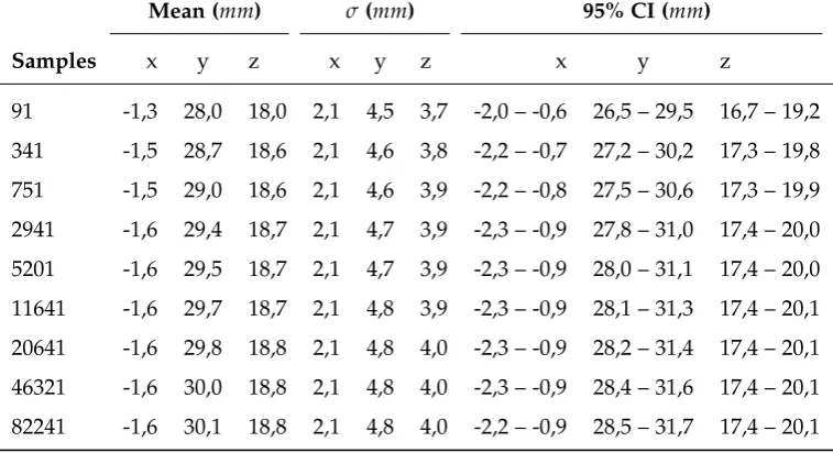
Table 5.3.1:The recalculated mean CCFP, standard deviation and 95% CI for the population of 36 patients for the skull in mm using various numbers of point samples with 128-grid simplification.

Mean (mm) σ(mm) 95% CI (mm)

Samples x y z x y z x y z

91 -1,3 28,0 18,0 2,1 4,5 3,7 -2,0 – -0,6 26,5 – 29,5 16,7 – 19,2 341 -1,5 28,7 18,6 2,1 4,6 3,8 -2,2 – -0,7 27,2 – 30,2 17,3 – 19,8 751 -1,5 29,0 18,6 2,1 4,6 3,9 -2,2 – -0,8 27,5 – 30,6 17,3 – 19,9 2941 -1,6 29,4 18,7 2,1 4,7 3,9 -2,3 – -0,9 27,8 – 31,0 17,4 – 20,0 5201 -1,6 29,5 18,7 2,1 4,7 3,9 -2,3 – -0,9 28,0 – 31,1 17,4 – 20,0 11641 -1,6 29,7 18,7 2,1 4,8 3,9 -2,3 – -0,9 28,1 – 31,3 17,4 – 20,1 20641 -1,6 29,8 18,8 2,1 4,8 4,0 -2,3 – -0,9 28,2 – 31,4 17,4 – 20,1 46321 -1,6 30,0 18,8 2,1 4,8 4,0 -2,3 – -0,9 28,4 – 31,6 17,4 – 20,1 82241 -1,6 30,1 18,8 2,1 4,8 4,0 -2,2 – -0,9 28,5 – 31,7 17,4 – 20,1

Table 5.3.2:The recalculated mean CCFP, standard deviation and 95% CI for the population of 36 patients for the skull in mm using various numbers of point samples with 256-grid simplification.

Mean (mm) σ(mm) 95% CI (mm)

Samples x y z x y z x y z

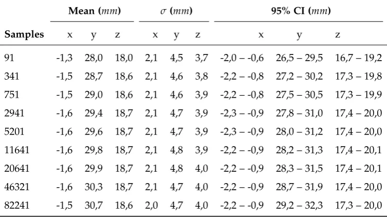
Table 5.3.3:The recalculated mean CCFP, standard deviation and 95% CI for the population of 36 patients for the skull in mm using various numbers of point samples without simplification.

Mean (mm) σ(mm) 95% CI (mm)

Samples x y z x y z x y z

91 -1,3 28,0 18,0 2,1 4,5 3,7 -2,0 – -0,6 26,5 – 29,5 16,7 – 19,2 341 -1,5 28,7 18,6 2,1 4,6 3,8 -2,2 – -0,8 27,2 – 30,2 17,3 – 19,8 751 -1,5 29,0 18,6 2,1 4,6 3,9 -2,2 – -0,8 27,5 – 30,5 17,3 – 19,9 2941 -1,6 29,4 18,7 2,1 4,7 3,9 -2,3 – -0,9 27,8 – 31,0 17,4 – 20,0 5201 -1,6 29,6 18,7 2,1 4,7 3,9 -2,3 – -0,9 28,0 – 31,2 17,4 – 20,0 11641 -1,6 29,8 18,7 2,1 4,8 3,9 -2,2 – -0,9 28,2 – 31,3 17,4 – 20,1 20641 -1,6 29,9 18,7 2,1 4,8 4,0 -2,2 – -0,9 28,3 – 31,5 17,4 – 20,1 46321 -1,6 30,3 18,7 2,1 4,7 4,0 -2,2 – -0,9 28,7 – 31,9 17,4 – 20,0 82241 -1,5 30,7 18,6 2,0 4,7 4,0 -2,2 – -0,9 29,2 – 32,3 17,3 – 20,0

Table 5.3.4:The original mean CCFP, standard deviation and 95% CI for the population of 36 patients for the skull in mm.

CCFP Mean (mm) σ 95%CI

Skullx 0.0 0.5 -0.3 – 0.1

Skully 29.9 4.6 28.3 – 31.5

Skullz 18.6 4.2 17.2 – 20.0

An effect of higher sampling is oversampling. Oversampling can result in a mesh consisting of more triangles than the original mesh that was sampled. The effect of oversampling can best be illustrated trough the number of duplicate face samples. In [Tables 5.3.5,5.3.6,5.3.7] the number and percentage of double samples is shown for each number of samples taken respectively for 128-grid, 256-grid and no simplification. Independent of the prior simplification there is only a small difference in double samples up to 5201 sampling. For 11641 and above there is an increasing difference in double samples between the levels of simplification varying from 1.0% to 40.8 %. The effect of the double samples on the CCFP position is limited as can be seen in [Tables 5.3.1,5.3.2,5.3.3]. As said earlier, up to 20641 samples there is a±0.1mm

Table 5.3.5:The timing and double samples per sampling after raycasting using 128-grid simplifiaction.

Samples Timing (s) Double samples

Raycast Gap fill CCFP Total (#) (%)

91 0.37 0.18 0.19 0.74 2 2.2 341 0.38 0.18 0.19 0.74 5 1.5 751 0.37 0.17 0.18 0.72 11 1.5 2941 0.38 0.19 0.19 0.75 37 1.3 5201 0.38 0.20 0.20 0.79 70 1.3 11641 0.38 0.22 0.21 0.82 304 2.6 20641 0.46 0.31 0.27 1.04 1361 6.6 46321 0.87 0.71 0.53 2.11 10392 22.4 82241 1.45 1.68 1.26 4.39 33520 40.8

Table 5.3.6:The timing and double samples per sampling after raycasting using 256-grid simplifiaction.

Samples Timing (s) Double samples

Raycast Gap fill CCFP Total (#) (%)

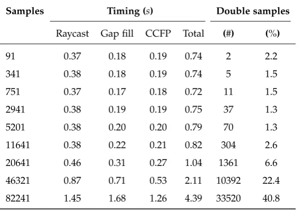
Table 5.3.7:The timing and double samples per sampling after raycasting using no simplifiaction.

Samples Timing (s) Double samples

Raycast Gap fill CCFP Total (#) (%)

91 3.15 0.16 0.17 3.49 2 2.2 341 3.16 0.16 0.17 3.49 5 1.5 751 3.10 0.16 0.16 3.43 10 1.3 2941 3.11 0.16 0.16 3.43 35 1.2 5201 3.36 0.18 0.18 3.72 59 1.1 11641 3.41 0.19 0.18 3.77 125 1.1 20641 4.03 0.29 0.25 4.57 216 1.0 46321 9.13 0.71 0.50 10.34 483 1.0 82241 16.52 1.68 1.19 19.39 1043 1.3

Finally there is computation time. We measured the most computational intensive tasks (Raycasting, Gap filling, CCFP calculation) for each number of sampling per simplification [Tables 5.3.5,5.3.6,5.3.7]. The simplification process in all cases was below 100msand therefor not reported. The total execution time for the 128-grid simplification is below one second up to 11641 samples. At 20641 samples this is just above one second. For 46321 and 82241 samples this is respectively 2.11 and 4.39 seconds. The 256-grid simplification starts at 1.28 seconds and increases to 1.81 seconds at 20641 samples. Again a bigger increase in computation time can be seen for the highest two forms of sampling up o 7.58 seconds. Using no simplification results in a 3.49 second execution time at the lowest sampling up to 19.39 seconds for the highest sampling. The primary cause for the increased execution time is the raycasting. Logically both the gap fill and CCFP computation show similar execution times for each form of sampling regardless of prior simplification due to processing the same amount of data.