Wind tunnel Investigation on Trailing Edge
Noise Mitigation via Sawtooth Serrations
C u s t o m e r
University of Twente
N a t i o n a l A e r o s p a c e L a b o r a t o r y N L R A n t h o n y F o k k e r w e g 2
CLASSIFIED
EXECUTIVE SUMMARY
CLASSIFIED Report no. NLR-TR-2014-310 Author(s)D. Engler Faleiros
Report classification
UNCLASSIFIED
Date
13-10-2014
Knowledge area(s)
Aëro-akoestisch en experimenteel aërodynamisch onderzoek Descriptor(s) Serrations Trailing Noise Acoustics
Wind tunnel Investigation on
Trailing Edge Noise Mitigation
via Sawtooth Serrations
Problem area
National Aerospace Laboratory NLR Anthony Fokkerweg 2, 1059 CM Amsterdam,
P.O. Box 90502, 1006 BM Amsterdam, The Netherlands
Telephone +31 (0)88 511 31 13, Fax +31 (0)88 511 32 10, Website: www.nlr.nl CLASSIFIED
Description of work
Enhance the potential of the use of sawtooth serrations on the trailing edge of wind turbine blades, in order to reduce noise at all frequency ranges, especially by investigating the influence of misalignment of the serrations with the flow.
Results and conclusions
Flexible serrations (FS) are more efficient than regular sawtooth serrations. Most of the high frequency noise previously reported in literature that was caused due to the application of serrations was eliminated. FS consistently showed great benefits with reductions up to 13 dB. Serrations, in general, decrease the aerodynamic efficiency and the pros and cons of using it need to be taken into account when considering full scale application.
Applicability
Serrations can be applied on wind turbine blades to decrease airfoil self-noise that occurs due to boundary-layer turbulence that passes over the trailing edge. This is the main noise mechanism of wind turbines, considering everything else is adequately treated.
Wind tunnel Investigation on
Trailing Edge Noise Mitigation
via Sawtooth Serrations
D. Engler Faleiros
C u s t o m e r
University of Twente
2 |
NLR-TR-2014-310No part of this report may be reproduced and/or disclosed in any form or by any means without the prior written permission of NLR (and contributing partners).
Customer University of Twente Contract number
Owner Not applied
Division NLR Aerospace Vehicles Distribution Limited
Classification of title Classified
Date 13-10-2014
Approved by:
Author
David Engler Faleiros
Reviewer Marthijn Tuinstra
Managing department Joost Hakkaart
NLR-TR-2014-310
|
3
Summary
This report investigates the performance of sawtooth serrations in mitigating
trailing edge noise from a DU-96-W-180 airfoil section, which is designed
especially for wind turbines. The experiments were realized at NLR’s Open-Jet
Anechoic KAT wind tunnel. Acoustic measurements were performed with a
48-microphone array. Aerodynamic experiments were done via hot-wire traverses
to obtain the boundary-layer and wake parameters.
The main conclusion of this work is that the use of a flexible mechanism, that
allows the serrations to auto-align with the flow, makes them effective over
almost the complete operational range. Furthermore, the high-frequency noise
penalty that was often reported in literature, no longer occurs. The hinge
mechanism that provides auto aligning with the flow should have a smooth
surface. The removal of material by making cuts inside the serrations was also
tested as a way of increasing flexibility. This concept however increased
significantly the produced noise.
Lastly, the mounting strategy in case of retro-fitting of an existing wind turbine
blade was investigated. Serrations fixed on the suction side of the airfoil
performed better than serration mounted on the pressure side.
NLR-TR-2014-310
|
5
Content
Abbreviations ... 7
List of Symbols ... 8
1
Introduction ... 10
1.1 Research Questions 11
2
Bluntness Noise ... 12
3
Full Scale to Wind Tunnel ... 13
4
Flow Similarity at the TE from the Acoustic Perspective ... 16
5
Serrations Design ... 18
5.1 Literature Review on Serrations 18 Discussion on literature reviewed 20 5.1.1 5.2 Hinge Mechanisms 21 5.3 Sawtooth Serration Models 25
6
Drag in the Far Wake ... 25
7
Experimental setup and test programs ... 31
7.1 Balance Measurements 31 7.2 Hot-wire 32 Boundary-Layer Measurements 32 7.2.1 Wake Measurements 32 7.2.2 7.3 Acoustic Measurements 33
8
Results ... 34
8.1 Lift Coefficients 34
8.2 Hot-wire 36
Boundary-Layer 36
8.2.1
Wake 38
8.2.2
8.3 Acoustics 41
Flexible Serrations 41
6
|
NLR-TR-2014-310Uncutted Serration Mounted on the Suction Side (US-TOP) 42 8.3.2
Uncutted Serration Mounted on the Pressure Side (US-BOT) 44 8.3.3
Cutted Serration (CS) and Serration with Cutted Plate (SCP) 44 8.3.4
9
Conclusions and Recommendations ... 45
9.1 Conclusions 45
9.2 Recommendations 46
Figures ... 47
NLR-TR-2014-310
|
7
Abbreviations
Acronym
Description
NLR National Aerospace Laboratory NLR
TE Trailing Edge
LE Leading Edge
BL Boundary Layer
TBL Turbulent Boundary Layer
LBL Laminar Boundary Layer
VS Vortex Shedding
SPL Sound Pressure Level
AoA Angle of Attack
Re Reynolds Number
Ma Mach Number
TBL-TE Turbulent Boundary Layer – Trailing Edge Noise TEB-VS Trailing Edge Bluntness – Vortex Shedding Noise
PNS Point of Noise Source
FS Flexible Serration
US-TOP Uncutted Serration fixed on the Suction Side (Top) US-BOT Uncutted Serration fixed on the Pressure Side (Bottom)
CS Cutted Serration
8
|
NLR-TR-2014-310List of Symbols
Symbol
Description
a Axial Induction Factor
a' Angular Induction Factor
αgeo Geometric Angle of Attack
αeff Effective Angle of Attack
b Half Width of the wake
B Number of Blades
c Chord Legth
c Speed of Sound
Cl Coefficient of Lift
Cd Coefficient of Drag
Cp Coefficient of Pressure
D’ Drag per unit span
δ Boundary Layer Thickness
δ* Displacement Thickness
FD Drag Force
FN Normal Force
FL Lift Force
h Half amplitude of the sawtooth serration
J’ Momentum per unit span
k Trip Height
L Wetted Span
ℒ Correlation length of the turbulence
λ Width of the sawtooth serration
λr Ratio of local tangential velocity and wind free stream velocity
M0 Mach Number of the undisturbed upstream flow
MV Component of the boundary layer Mach Number perpendicular to the
edge
μ Dynamic Viscosity
ν Internal angle between height and side of the serration
ν Kinematic viscosity
Ω or ω Rotational Speed of the blade
〈𝒑𝟐〉 Mean-square sound pressure at the observer
ρ0 Medium fluid density
ρ Density of the fluid
ϕ Angle of the serration with the chord line
ϕ Relative Wind Angle
NLR-TR-2014-310
|
9
Ѱ0 Nondimensional edge noise spectrum in the absence of the serration
Q Torque
r Distance from the edge to the observer
r/R Ratio of radius location at the blade an the total blade radius
t Trailing Edge Thinkness
T Thrust
θ Pitch Angle
θtop Angle at the TE between the airfoil top surface and the chord line
θbot Angle at the TE between the airfoil bottom surface and the chord line
u Local velocity in stramwise direction
u1 Velocity deficit
𝒖
̅ Temporal mean velocity in streamwise direction
U Velocity
Uc Convection Velocity
𝐔∞ Free Stream Velocity
𝐔𝒆 Edge Velocity
v Local velocity in transverse direction
v Tangential Velocity
v’ Turbulent transverse velocity
v'² Mean-square turbulence velocity
10
|
NLR-TR-2014-3101
Introduction
On a wind turbine different noise sources can be identified, such as hub noise or the noise generated by the blades moving through the air. Studies performed by other authors showed that aeroacoustic noise is most relevant, provided that all the other ones are adequately treated
(1).The aerodynamic sources are divided into two main groups: inflow-turbulence noise, which is caused by upstream turbulent flow around the Leading Edge (LE), and airfoil self-noise (2), which is caused by the interaction between the airfoil blade and the turbulence produced in its own boundary layer and near wake (3).
The airfoil self-noise mechanisms are (3):
Turbulent Boundary Layer – Trailing Edge (TBL-TE) Noise, caused by the interaction between the TBL and the TE;
Laminar Boundary Layer – Vortex Shedding (LBL-VS) Noise, which is caused by large LBL,
whose instabilities result in Vortex Shedding (VS) at the Trailing Edge (TE);
Flow separation close to the TE on the suction side for small angles of attack (AoA), producing noise due to shed turbulent vorticity;
Deep Stall (high AoA), causing the airfoil to radiate low-frequency noise, similar to a blunt body;
And Trailing Edge Bluntness – Vortex Shedding (TEB-VS) Noise, which is noise generated due to VS at a blunt TE.
Wind turbines extract power from the wind at relatively low wind velocities, from 7.5 m/s to 10 m/s in average. However, when taking into account the rotation of the blades, the relative velocity of the blades can become ten times higher or more, depending on the rotational speed and on the spanwise location at the blade. Thus, Reynolds Numbers based on chord length of O(106) are achieved and a TBL (Turbulent Boundary Layer) develops over the blade. Therefore, as long as separation does not occur and the TE is sufficiently sharp to avoid bluntness noise, TBL-TE noise is the dominant mechanism.
According to Howe (4), at right angles to the flow, the edge noise scales with 𝐿ℒ𝑉5(1 − 𝑀0−
𝑀𝑉1), where L is the wetted span, ℒ the correlation length of the turbulence parallel to the edge, V the characteristic edge convection velocity, M0 the undisturbed upstream flow Mach Number
NLR-TR-2014-310
|
11
The attenuation of noise by serrations may be attributed to an effective reduction of the
spanwise length at the trailing edge that actually contributes to the generation of sound, even
though the physical wetted length increases with the serrations (5). It is derived in Howe (6) for
sawtooth serrations that
Ψ(ω) ≈ Ψ0(ω)
[ 1 + (4ℎ𝜆 )2]
, λ
h< 1, 𝜔ℎ
𝑈 ≫ 1 (1)
where 𝛹(𝜔) is the nondimensional edge noise spectrum, 𝛹0(𝜔) is the noise in absence of the
serration, ω the acoustic frequency, U is the main stream velocity and λ/h is the width over the
half amplitude of the serrations (Figure 1). Therefore, if the ratio λ/h is reduced the attenuation
of noise increases, i.e. slender serrations are more effective.
Nonetheless, experimental investigations show that Howe’s prediction overestimates the amount of noise that can be reduced (7; 8) and that noise reductions are also obtained at low frequencies. According to these studies, sawtooth serrations presented low to mid frequencies moderate TBL-TE noise reduction up to 7dB and even increased the amount of TBL-VS noise at high frequencies. The misalignment of the serrations with the flow was suggested, e.g. by Braun
(9), as a possible cause of noise level increase at high frequencies.
The objective of this report is to verify the impact of sawtooth serrations on TE noise mitigation on a wind turbine blade, with different configurations. The most important point of this study was to attempt to improve noise reduction via mechanisms that allow auto-alignment of the sawtooth serrations with the flow. Experimental investigations were carried out in the NLR’s Small Anechoic Wind Tunnel (KAT) on a DU-96-W-180 airfoil, which is specifically designed for wind turbine applications (10).
1.1
Research Questions
The research questions that motivated this experimental investigation are:
1) How much noise can be mitigated from the airfoil DU-96-W-180 by the use of serrations?
2) Does the alignment of the serrations affect the amount of sound reduced? 3) Is the aerodynamic efficiency of the airfoil affected by the use of serrations?
12
|
NLR-TR-2014-310Before starting the experiments, there were other definitions to be made in order to accomplish a relevant investigation:
a) Which part of the blade should be studied? b) Is it necessary to apply trips in the airfoil?
c) What should be the dimensions of the serrations (λ/h) to maximize the noise reduction? d) What mechanisms can be used to auto-align serrations with the flow?
e) How to evaluate the aerodynamic efficiency of the airfoil?
Chapter 2 discusses the presence of bluntness noise. Chapter 3 makes a comparison between the model scale and the full scale. Chapter 4 discusses the flow similarity at the trailing edge from an acoustic perspective. Chapter 5 show some literature review and simulations performed that led to the serration models to be tested. Chapter 6 explains how drag can be calculated from the wake, derive the equations and show some simulations of the wake development. Chapter 7 describes the experiments setup and test programs. In the Chapter 8, the results are presented. And finally, in Chapter 9 the conclusions and recommendations are presented.
2
Bluntness Noise
A description of the noise mechanisms was done in the introduction and a more detailed description was done by Brooks et al (3). With high wind tunnel speeds and small angles of attack, the presences of fully laminar BL or strong separation are not a concern. Turbulent boundary-layers are present in all conditions tested and are the dominant noise mechanism. Bluntness noise due to a TE with finite thickness is discussed in this section.
Empirical evidence (11) shows that for t/δ* < 0.3 bluntness noise can be neglected. The thickness of the TE is small (t/c = 0.0027) and its ratio with the displacement thickness δ*at different conditions were simulated using Xfoil, which is an interactive program for the design and analysis of subsonic isolated airfoils (12). The results are shown in Table 1. Angles of attack were varied from 0° until 9° and the free stream velocities simulated are 70 m/s, 40 m/s and 20 m/s for an airfoil of 0.15 m chord. In this table only δ*top is considered. If δ*bot had been added to the total
δ* the ratios t/δ* values would be even smaller.
TE thickness over displacement thickness (t/δ*
top)
AoA
70 m/s
40 m/s
20 m/s
NLR-TR-2014-310
|
13
1°
0.26
0.22
0.16
2°
0.24
0.20
0.15
3°
0.22
0.19
0.13
4°
0.20
0.17
0.12
5°
0.18
0.16
0.11
6°
0.16
0.14
0.09
7°
0.15
0.13
0.09
8°
0.13
0.11
0.09
9°
0.10
0.10
0.08
Table 1 – Bluntness Factor t/ δ* simulated in the Xfoil
These results show that bluntness noise can be neglected. However, during the experiments serrations were inserted in the trailing edge of the airfoils, which change the nature of the flow at that region. Thus, there is still a possibility that bluntness noise is present in the serrated configurations.
3
Full Scale to Wind Tunnel
Flow similarity is an important parameter in an experimental investigation, not only to translate the wind tunnel results into practical wind turbines conditions, but also to provide information on characteristics that must be present in the experiment. Two non-dimensional parameters define if one flow can be considered similar to another. The Re (Reynolds Number)
Re =ρ𝑈∞c
μ =
𝑖𝑛𝑒𝑟𝑡𝑖𝑎𝑙 𝑓𝑜𝑟𝑐𝑒𝑠
𝑣𝑖𝑠𝑐𝑜𝑢𝑠 𝑓𝑜𝑟𝑐𝑒𝑠 (2)
where ρ is the density, μ is the dynamic viscosity 𝑈∞ is the free stream velocity and c is the chord length. And the Ma (Mach Number)
Ma =𝑈∞
c (3)
where c is the speed of sound.
14
|
NLR-TR-2014-310turbulence intensity and the boundary layer (BL) thickness are different at the TE in these two cases.
The Mach Number does not play a vital role here, since the velocities in the wind tunnel are not very different from the real flow condition and the rule of thumb for Ma < 0.3 here applies and the assumption that the flow is imcompressible is used.
In the experiments a 2D situation is investigated (i.e. a section of an airfoil spanned across the wind tunnel section). On a wind turbine the flow is 3D and the cross sections of the blade vary in chord length and also in the twist angle. The relative wind speed and subsequently the Re also change through the blade as a function of span. Consequently, natural transition will be located in different points and the boundary layer characteristics will vary. Hence, when studying an airfoil for wind turbine purposes one region needs to be chosen that represents a section of the blade. Since most of the noise is produced on the 25% outer part of the blade (12), this is the focus here. Specifically it was chosen to work with a blade section at 90% span (r/R = 0.9).
Using generic design rules for a wind turbine blade the typical chord length and the relative velocity at that section was assessed. For this, it was used Blade Element Momentum (BEM) Theory, as it is described in the book ‘Wind Energy Explained’ (13). The following assumptions are made in order to simplify the calculations:
No rotor plane deflection with the wind;
Wake rotation is not considered (a’ = 0);
There is no drag, 𝐶𝑑= 0;
Effects of tip vortices and downwash are not considered;
The axial induction factor a = 1/3.
With the above assumptions the following relations are derived (13):
𝜑 = tan−1 2
3𝜆𝑟 (4)
𝑈𝑟𝑒𝑙 = 2/3 ( 𝑈
sin 𝜑 ) (5)
𝑐 =8𝜋𝑟 sin 𝜑
NLR-TR-2014-310
|
15
Where 𝜑 is the angle of relative velocity, 𝜆𝑟= 𝜔𝑟/𝑈 is the ratio of tangential and free stream velocity, 𝑈𝑟𝑒𝑙 is the relative wind velocity, c is chord length and B is the number of blades (B=3).
Using data from a typical wind turbine of 2MW and the Equations 4, 5 and 6 the chord length and consequently the Re were determined. The data used and calculations are summarized at the
Table 2.
Reference Reynolds Number at Wind Turbine Conditions
Rotational Speed (rpm) 19.0
Rotational Speed - ω (rad/s) 2.0
Rotor Radius - R (m) 45.00
Local radius Position - r (m) 40.50
Tangential Velocity at r - v (m/s) 81.00
IEC Wind Class IIA
Wind Average Speed - U (m/s) 8.5
Axial Induction factor - a 1/3
λr = v/U 9.53
Angle of relative wind ϕ (rad) 0.070
Angle of relative wind ϕ (degrees) 4.00
Relative Velocity - Urel (m/s) 80.39
Lift Coefficient - Cl 1
Number of Blades - B 3
Chord Length at r (m) 0.85
Density of Air - ρ (kg/m³) 1.225
Dynamic Viscosity of Air - μ 1.8E-05
Reynolds Number at r 4.5E+06
Table 2- Chord Length and Reynolds Number Calculation for the airfoil section at r/R = 0.9
16
|
NLR-TR-2014-3104
Flow Similarity at the TE from the Acoustic
Perspective
As explained in the last section, it is not possible to achieve full similarity between model scale
and full scale, since the maximum Re achieved at the wind tunnel is six times lower than
required. Ffowcs Williams and Hall’s theory (14) applied to the problem of turbulence convecting
at low subsonic velocity Uc above a large plate and past the trailing edge into the wake yields as a
primary result (3)
〈𝑝2〉 ∝ 𝜌 02𝑣′2
𝑈𝑐3
𝑐 ( 𝐿ℒ
𝑟2) 𝐷̅ (6)
where ρ0 is the medium density, v’² is the mean-square turbulence intensity velocity, c is the
speed of sound, L is the spanwise extent wetted by the flow, ℒ is a characteristic turbulence
correlation scale, r is the distance from the edge to the observer and 𝐷̅ is the directivity factor,
which equals 1 for observers normal to the surface from the leading edge. The usual assumptions for the boundary layer flow (3) are that 𝑣′∝ 𝑈𝑐 ∝ 𝑈∞ and ℒ ∝ 𝛿 𝑜𝑟 𝛿∗. Thus, trailing edge noise scales with 𝑈∞5𝛿∗. Comparing noise emission between model and full scale, these two parameters should be similar in both flows. 𝑈∞ is approximately the same at model and full scale
and δ* in both cases are compared in this section.
According to Boundary-Layer Theory (15)the BL thickness δx at a specific point x/c should grow
while decreasing the Reynolds Number, given that in both situations they have the same nature (laminar or turbulent). This is because for lower Re the viscous forces start to play a more fundamental role than the inertia forces (Equation 2), causing the BL thickness to increase. A second effect on the BL thickness is that a TBL grows faster with x than a laminar one (15). For instance, a TBL thickness in a flat plate grows proportionally to x0.8, while a LBL (laminar BL) grows proportionally to x0.5. For higher Re transition occurs earlier and therefore δTE (BL thickness at the
TE) increases with Re. With these two effects acting together, one increasing and the other decreasing δ with Re, it was uncertain whether the BL thickness would be smaller or bigger in the wind tunnel. Thus, simulations on the Airfoil DU-96-W-180 were required, which were performed using Xfoil.
NLR-TR-2014-310
|
17
effective and actual shapes is equal to the local displacement thickness δ*. This is only about 1/3 to 1/2 as large as the overall boundary layer thickness.
Figure 2 shows that for a fixed transition position and AoA = 8.2°, the displacement thickness δ* (and consequently δ) reduces with Re. This plot was made for the suction side, where Re = 0.72×10⁶ corresponds to the situation in the wind tunnel (c = 0.15 m and U = 70 m/s) and Re = 4.5×10⁶ to the wind turbine. Comparing these two cases, δ* almost halved.
Figure 3 shows δ* when natural transition occurs. After Re = 1.7×10⁶, the effect of the boundary layer increasing due to turbulent flow starts to dominate. One can see in Figure 4 that the transition point on the suction side reduces with increasing Re, i.e. the transition occurs closer to the LE. Therefore, the higher the Re the bigger the turbulent region is.
In Figure 3, δ* = 0.022 for both Re of interest at AoA = 8.2°, which is the ideal case for flow similarity. Indeed, δ* was first plotted for Re = 0.72×10⁶ (model scale) and Re = 4.5×10⁶ (full scale) at various AoA (Figure 5). There is a region between AoA = 8.2° and AoA = 10.5° where the δ* is
similar for both flows. Hence, working with AoA = 8.2° provides the flow similarity required for
the acoustic measurements. Moreover, δ* = 0.02 and AoA = 8° are typical values found in wind
turbines in the region closer to the blade tip, according to NLR’s confidential database. Thus,
working at this angle also provides insight on the region of interest (r/R = 0.9).
For angles below 8.2°, the boundary layer thickness is already thicker in the wind tunnel than in
the full scale. The technique of tripping, used in other experiments (17) to force transition, would
only increase δ* even more. Going further than 8.2° (effective AoA) would be a problem in noise
investigation because of the deflection of the jet by the airfoil in the open-jet wind tunnel outside
the collector, which would cause an extra background noise. Finally, it is also important to realize
that at AoA = 8.2° and Re = 0.72×10⁶, natural transition on both sides of the airfoil occurs, which
is crucial for the analysis of TBL-TE (Turbulent Boundary Layer - Trailing Edge) noise.
Lower velocities were also tested and they also showed good approximation at a region close to
8.2°.The possibility of using c = 0.20 m (Re=0.96×10⁶) was also verified, but yielded only a minor
improvement. Since the lift increases, the flow deflection would increase, which could demand a
reduction in flow velocity or angle of attack. Thus, chord length of 0.15 meters remained as the
18
|
NLR-TR-2014-3105
Serrations Design
This section is divided in three parts. The first is a literature review on typical serrations that has been tested and the conclusions that were drawn by the authors. The second talks about hinge mechanisms, which were applied in the root of some serrations in order to enable auto-alignment with the flow. The third part presents the final models of the serrations which were selected for the experiments.
5.1
Literature Review on Serrations
Theoretical investigation pointed out that the serration geometry determines the magnitude of
the noise reduction (6). In theory, noise reduction is expected to increase as λ∕h (width over half
length) decreases, meaning that narrow serrations are predicted to outperform wide serrations
in terms of noise attenuation at all frequencies and flow speeds.
Moreau & Doolan (7) used a flat plate model at 0° AoA and with low and moderate Re in their
study. Three configurations with 0.5 mm thick trailing edge plates were tested: a straight
unserrated configuration, a narrow serration (λ/h = 0.2) and a wide serration (λ/h = 0.6). The
frequency range in the analysis was separated using the non-dimensional Strouhal Number,
based on the BL thickness, Stδ = fδ/U. The narrow serrations (Table 3) reduced noise up to 2.5 dB
at region R1 (Stδ < 0.13), increased the noise up to 3dB at region R2 (0.13 < Stδ < 0.7) and reduced
up to 10 dB of blunt vortex-shedding noise at R3 (0.7 < Stδ < 1.4). The wide serrations (Table 4)
reduced noise up to 3 dB at region R1 (Stδ < 0.2), barely changed at region R4 (0.2 < Stδ < 0.7) and
reduced up to 13 dB of blunt vortex-shedding noise at R3 (0.7 < Stδ < 1.4). In general, wider
serrations outperformed the wider ones.
Serration λ/h λ (mm) h (mm) R1 (Stδ < 0.13)
R2
(0.13 < Stδ < 0.7)
R3
(0.7 < Stδ < 1.4)
Narrow 0.2 3 15 ↓2.5 dB ↑3 dB ↓10 dB
Table 3 – Narrow Serrations Results from Moreau & Doolan (2003)
Serration λ/h λ (mm) h (mm) R1 (Stδ < 0.2)
R4
(0.2 < Stδ < 0.7)
R3
(0.7 < Stδ < 1.4)
Wide 0.6 9 15 ↓3 dB 0 dB ↓13 dB
Table 4 – Wide Serrations Results from Moreau & Doolan (2003)
Gruber et al (8) did extensive work on sawtooth serrations applied to the airfoil NACA 651-210.
NLR-TR-2014-310
|
19
mm for both h = 10 mm and h = 15 mm (halve lengths). For this case, the narrowest serrations,
with λ = 1.5 mm and λ = 3 mm, gave the best results at middle frequencies (300Hz < f < 7000Hz)
with a reduction up to 5dB for h = 10 mm and 7dB for h = 15mm. For higher frequencies all
serrations increased the noise levels, being higher for smaller λ and with maximum of 3dB. In the
second part the authors fixed λ = 3 mm and varied h between 1 and 40 mm, building up a total of
27 sawtooth configurations. One important finding is that a sawtooth with root-to-tip distance
smaller than the boundary layer thickness is inefficient in noise reduction, i.e. h/δ should be
higher than 0.5. The frequency range where serrations were efficient to reduce noise was
reported to be in the range 0.5 < Stδ < 1, where Stδ = fδ/U. Gruber et al agreed with Howe’s
theory in the sense that the sharper the serration, the more noise is reduced. Finally, they
showed by flow visualization that there is crossflow within the teeth of the sawtooth serrations,
which the authors considered to be the cause of high frequency noise generation.
Braun et al (9), realized experiments with sawtooth serrations in six different configurations
which included λ/h of 0.33, 0.67 and 1 and serrations with different alignment angles with the
suction side, which the authors called straight, bent and curved. For these configurations they
tested AoA from 0 to 14°. The results found by Braun et al are summarized in the Table 5
considering AoA from 6° to 8°. The results are not discrete as presented here, since for a
continuous range of frequencies and AoA it is difficult to summarize with a unique value.
Nevertheless, the table gives a good summary, which helps to understand some important
conclusions from Braun:
A reduction from 2 to 3.5 dB was found to occur in low frequencies and medium AoA.
Serrations aligned with the suction side of the airfoil increased the noise production in
high frequencies.
Aligning the serrations with the flow at the TE by curving or bending the serration,
caused reduction of noise in high frequencies as well.
Serration* λ/h λ (mm) h (mm) Geometry Low Freq. (0.63 -2 kHz)
Medium Freq.
(2 - 4 kHz)
High Freq.
(4 - 6 kHz)
Straight 2:1 1.00 20 20 Straight ↓2 dB ↑6 dB ↑8 dB
Straight 6:1 0.33 6.66 20 Straight ↓2 dB ↑6 dB ↑8 dB
Curved 2:1 1.00 20 20 Curved ↓3.5 dB ↓4 dB ↓2 dB
Bent 2:1 1.00 20 20 Bent ↓3 dB ↓3 dB ↓2 dB
Bent 3:1 0.67 20 30 Bent ↓3.5 dB ↓3 dB ↓3 dB
Table 5 - Results from Braun et al for different types of serrations
20
|
NLR-TR-2014-310One conclusion from Braun that is not apparent from the table is that in the range of frequencies around 1 kHz for almost all configurations, a tone appeared, reducing the absolute noise reduction benefit. Lastly, it is important to emphasize is that the work from Braun et al argues that the misalignment of the serration with the flow is what causes noise increase at high
frequency. These findings support the idea for testing flexible serrations in this project.
Discussion on literature reviewed
5.1.1
Moreau and Doolan obtained significant reductions in high frequencies, however it should be noted that those were attenuations of bluntness noise, which apparently was not present in the other studies.
Moreau and Doolan found contradictory results compared to Gruber et al in respect to whether narrow or wide serrations perform better. Though, a possible reason is that the former used a flat plate and the latter analysed an airfoil. Besides, when looking into the whole data of Gruber et al, one can find trends and draw conclusions, however when comparing the serrations in pairs, it is sometimes unclear if a wide or a narrow serration performs better. As discussed by Gruber et al, it is uncertain if the ratio λ/h is the independent variable to be analysed or if h and λ should be verified separately. One guideline to be followed is that h should be bigger than δ. Another appears to be that sharper serrations gives better noise reduction until Stδ = 1, at least for airfoils. However it should not be too sharp since in this case high frequency noise can be produced.
Finally, the ratio for the sawtooth serrations chosen for this experimental investigation is λ/h =
0.5. To support this decision Figure 6 from Gruber et al (8) is reproduced here. In the figure, it is
shown the difference in sound power level ΔPWL in third octave bands and within limits of +- 2
dB. The experimental parameters are AoA = 5° and U = 60 m/s (Re = 0.62×10⁶). For λ/h = 0.5 (h/λ
= 2 in the figure) reductions on the radiated sound are obtained in the range 0.3 < Stδ < 0.8, while
for Stδ > 0.8 noise increase is not relevant. Thus, λ/h = 0.5 appears to be an adequate choice.
Besides, the investigation here reported focused on other aspects of the serrations than to find
the most optimal ratio λ/h.
The sawtooth amplitude was calculated as h = 5δ*, in order to obtain h/δ ~ 1, assuming that δ ~
5δ*. Therefore, the half length and width of the sawtooth used in the experiments are,
NLR-TR-2014-310
|
21
5.2
Hinge Mechanisms
According to Braun (1998), aligning the serrations with the flow by bending them, can be a solution for the noise increase caused by serrations in high frequency band. However, only bending them would not completely solve the problem as the AoA is not always constant during the operation of a wind turbine. For instance, the blade is rotated around its own axis in order to apply pitch control for the purpose of adjusting the output power. The solution then appears to be increasing the flexibility of the serrations, allowing it to auto-align with the flow when a new AoA is imposed.
To define the initial bent position, Xfoil simulations were performed at AoA = 8.2° and Re = 0.72×10⁶. In order to do so, first a 3 cm plate extension was included into the Airfoil geometry in Xfoil, aligned with the chord line ϕ = 0°, where ϕ is the angle between the serration and chord line. This is only an approximation method, since Xfoil only simulate 2D flow and does not consider 3D effects caused by a serrated profile. In this manner, a graph of Cp vs. x/c was
obtained and the torque around the trailing edge was calculated.
Different angles ϕ were evaluated until the orientation where the torque equals zero was found at ϕ = 2.1° (Figure 7). The pressure distribution on the 2D serration, obtained in the Xfoil can be seen in Figure 8. The same routine was realized for a second configuration, in which a plate length of 3.6 mm was added between the serrations and the airfoil TE, increasing the torque around the TE. The 3.6 mm length is part of one of the tested serrations which is explained later in this section in more details. For this new configuration, ϕ = 2.3° was obtained. From these values the bent angles for pressure or suction side mounting were derived. In order to do so, the internal angles close to the trailing edge θtop (top side) and θbot (bottom side) were taken into
account (Figure 9).
In Table 6, the values for the bending angle between the serration and the chord line ϕ for the regular serration (ϕser) and for the serration with a plate of 3.6 mm preceding the serration (ϕpla)
are given.
θ
topθ
botϕ
serϕ
plaϕ
ser+ θ
topϕ
pla+ θ
topθ
bot- ϕ
ser13.0° 3.9° 2.1° 2.3° 15.1° 15.3° 1.8°
Table 6 – Bent Angles for the serrations
22
|
NLR-TR-2014-310angle is tested, such as AoA = 0°, a torque is experienced (Figure 10). The use of a serration that auto-aligns with the flow through a hinge mechanism is therefore considered.
Two different methods were used as a way of improving the flexibility of the serrations. One of them is a mechanical hinge mechanism created by laser cutting the sawtooth serrations, in such a way that separated small beams are shaped in the metal sheet, close to the root of the teeth. Through torsion these small bars twist and the serrations can pivot around the TE. This first technique is the basis of two different serrations, which will be referenced with the term “cutted”, to indicate that the laser cuttings are present. Another approach is to create a hinge by connecting the serrations to the trailing edge via a flexible material, such as adhesive tape. This latter method is referenced to as Flexible Serrations (FS).
In order to design the laser cuts, some basic solid mechanics modelling was performed. The Assumption is that the beam in which torsion occurs is only formed by the spring connection l between structural connections which would only act as links (Figure 11). The total torque acting on one spring connection is given by (18):
𝑇 =𝜃𝐺𝐽
′
𝑙 (7)
Where θ is the angle which one spring connection turns when torque is applied, G is the torsional modulus for steel (~77 GPa) and J’ the polar moment of inertia. For a solid rectangular section
with side 2a and thickness 2b, J’ is defined by (18)
𝐽′= 𝑎𝑏3[16
3 − 3.36 𝑏 𝑎(1 −
𝑏4
12𝑎4)] (8)
in which a ≥ b. The total bent angle of the serration due to torsion is then defined as:
𝛩 = 𝜃. 𝑛
(9)
NLR-TR-2014-310
|
23
ground. Furthermore, the weight is one order of magnitude lower than that due the torque applied by the flow.
Using a Matlab program, predictions were carried out on the flexibility of each serration concept in order to design the hinge layout. The thicknesses (2b) of the material tested were 0.3, 0.4 and 0.5 mm. The distance between the cuts (2a) was set as 0.6 mm, because it was the maximum precision that could be obtained in the workshop. J’ was then calculated for each half thickness b. Then, the number n of springs was plotted against the connection length l for each model of serration. The first prototype simulated was the one with laser cuts inside the serration. From now one, this model will be referenced here as Cutted Serration (CS) (Figure 13). In this case, the maximum spring beam size is determined by the width of the serration. Furthermore, the number of springs is restricted, because the surface of the serration cannot be completely covered with cuts. Therefore, a choice was made of n = 6, to provide a hinge that covers 14% of the surface of the serration at maximum.
The results for the Cutted Serration are plotted in Figure 16. The objective was to verify how much deflection could be obtained for the l and n parameters that are defined by the serration geometry. Notice that the spring length l is not constant for this concept and it is reduced when moving towards the tip of the sawtooth serration, because of its triangle shape. Therefore, in the
Figure 16 the horizontal axis represents the average length of the connection, which for n = 6 is l = 1.4 mm. Figure 16 shows that t = 0.3 mm, l = 1.4 mm and n = 6 is a viable solution for a total bending of 𝛩 = 0.8°.
The second concept includes a small plate of 3.6 mm before the serrations to facilitate the hinge mechanism. The length of 3.6 mm was chosen in order to make it possible at least four springs. This way, the serration was freed from cuts in the triangle area. This model is referenced as Serration with Cutted Plate (SCP) (Figure 14). In this case,n = 4 and l = 5.1 mm. The maximum
bending was 𝛩 = 3.2° (Figure 17).
However, what is the required angle at which a serration should be able to bend as to fully align with the flow? Considering the range of AoA from 0° to 8.2°, this range of angles ϕ was estimated using Xfoil as follows:
Applying AoA = 0° and U = 70 m/s, it was found that ϕCS/US, α=0° = -2° and ϕSCP, α=0° = -1.5°
24
|
NLR-TR-2014-310 Comparing these neutral positions with the ϕ values found before for AoA = 8.2° (ϕCS/US,α=8.2° = 2.1° and ϕSCP,α = 2.3°) it was estimated that the serration should be able to
pivot 4.1° and 3.8° around the TE for CS/US and for SCP models, respectively.
Therefore, the simulations show that SCP should be able to align with the flow in 85% of the range (3.1° of 3.8°) from 0° to 8.2°, while for CS only 20% (0.8° of 4.2°). Even though it is not as efficient as required, any gain in flexibility should represent some noise reduction, at least at angles close to 8.2°, which is the AoA in which the serrations are designed to be initially aligned.
The simulations done here have some limitations such as the fact that Xfoil is 2D flow simulator and also the fact that only torsion was considered and not bending. This latter phenomenon would probably help the serrations to better align with the flow, increasing the deflection and giving a slightly curved profile. However, it was assumed here that torsion is the most influent phenomena and responsible for most part of the serration rotation.
The reference torque values used in the simulations were also compared with the maximum torques supported by the internal beams and it was confirmed that the torsional stress caused by the air is below the maximum stress the material can handle without plastic deformation to occur. The maximum stress at the midpoint of one beam with a solid rectangular section is (18):
𝜏𝑚𝑎𝑥 =
3𝑇𝑚𝑎𝑥
8𝑎𝑏2 [1 + 0.6095 (
𝑏
𝑎) + 0.8865 ( 𝑏 𝑎)
2
− 1.8023 (𝑏 𝑎)
3
+ 0.9100 (𝑏 𝑎)
4
] (10)
So, using 58% of the yield stress (Von Mises Criterion) of stainless steel (~520Mpa) the maximum torque that one beam can hold depending on b (half thickness) and a (half distance between cuts) were calculated (Table 7).
Torque Simulated in Xfoil (Maximum at AoA = 0°)
US or CS 0.0005 Nm
SCP 0.0016 Nm
Maximum Torque supported depending on thickness
t = 0.3 mm 0.0040 Nm
t = 0.4 mm 0.0067 Nm
t = 0.5 mm 0.0099 Nm
NLR-TR-2014-310
|
25
5.3
Sawtooth Serration Models
Until this section it was discussed all the theory used and simulations performed to define the serration models to be tested. In this section it is summarized the models to be tested:
Clean Configuration (just the airfoil without serrations);
Uncutted Serration fixed on the suction side (US-TOP) (Figure 12 A1);
Uncutted Serration fixed on the bottom side (US-BOT); (Figure 12 A2); Cutted Serration (CS) (Figure 13);
Serration with Cutted Plate (SCP) (Figure 14);
Flexible Serration (FS) (Figure 15);
6
Drag in the Far Wake
This section explains how the drag on an airfoil is calculated in the far wake of an airfoil, which helps to answer the question: “Is the aerodynamic efficiency of the airfoil significantly affected by the use of serrations?” Moreover, the width increase of the wake moving downstream from the TE is estimated, to determine the measuring locations in the experiments.
A wake is a so-called free turbulent flow, because it is not confined by a solid wall. It is formed behind a body that is being dragged in a fluid at rest or behind a body which has been placed in a stream fluid. The velocities in the wake are smaller than the edge velocity, due to momentum losses, caused by airfoil drag. The width of the wake increases as it moves away from the body and the deficit velocity decreases. The drag in the body can then be calculated through the momentum equation (15).
26
|
NLR-TR-2014-310The velocity depression behind the wake is expressed as the difference between the stream velocity and the flow velocity, being the depression maximum at the center of the wake and zero in the half width b, where 𝑢1= 𝑈∞. Thus, the velocity depression is defined as
𝑢1= (𝑈∞− 𝑢) (11)
where 𝑈∞ is the free stream velocity and u the local velocity in the wake. Problems in free turbulent flow are of boundary-layer nature. This means that the region in the space where the solution is being pursued does not extend far in the transverse direction, as compared with the main direction of the flow and that transverse gradients are large compared to gradients in streamwise direction. Consequently it is permissible to study such problems using the boundary-layer equations. In two-dimensional motion, neglecting compressibility effects the momentum equation is then given by
𝜕𝑢 𝜕𝑡+ 𝑢
𝜕𝑢 𝜕𝑥+ 𝑣
𝜕𝑢 𝜕𝑦= 1 𝜌 𝜕𝜏 𝜕𝑦 (12)
and continuity by
𝜕𝑢 𝜕𝑥+
𝜕𝑣
𝜕𝑦= 0 (13)
where x is the streamwise direction, y is the transverse direction and u and v the local velocities
at x and y directions, respectively.
Prandtl’s mixing-length hypothesis allows expressing the shear stress as follows
𝜏 = 𝜌𝑙2|𝑑𝑢
𝑑𝑦| 𝑑𝑢
𝑑𝑦 (14)
where 𝑢̅ is temporal mean velocity in x direction, ρ is the density of the fluid and l is the so-called mixing length. Furthermore, in the far wake of 2D flow the term 𝑣𝜕𝑢/𝜕𝑦 is small and can be neglected. Hence, assuming steady flow and substituting (11) and (14) in (12) yields
−𝑈∞
𝜕𝑢1
𝜕𝑥 = 𝑙2 𝜕𝑢1
𝜕𝑦 𝜕2𝑢
1
𝜕𝑦2 (15)
When dealing with turbulent wakes it is usually assumed that l is proportional to the width of the wake 2b. Hence:
𝑙
NLR-TR-2014-310
|
27
Additionally the following rule endured with time:
𝐷𝑏 𝐷𝑡~ 𝑣′
This equation states that the rate of increase of the half width b is proportional to the transverse turbulent velocity v’. In Prandtl’s mixing-length theory, it was derived that:
𝑣′~𝑙𝜕𝑢
𝜕𝑦
Thus:
𝐷𝑏 𝐷𝑡~ 𝑙
𝜕𝑢 𝜕𝑦
The mean value of 𝜕𝑢/𝜕𝑦 taken over half of the width of the wake is assumed to be proportional to 𝑢1/𝑏. So,
𝐷𝑏
𝐷𝑡 = 𝑐𝑜𝑛𝑠𝑡 × 𝛽𝑢1 (16)
Now, using the definition of the material derivative:
𝐷𝑏 𝐷𝑡 =
𝜕𝑏 𝜕𝑡+ 𝑢𝑖
𝜕𝑏 𝜕𝑥𝑖
Using assumption of steady state and since b is only function of x:
𝐷𝑏 𝐷𝑡 = 𝑢
𝑑𝑏
𝑑𝑥 (17)
So, because 𝑢=(𝑈∞− 𝑢1) and under the assumption (𝑢1≪ 𝑈∞):
𝐷𝑏 𝐷𝑡 = 𝑈∞
𝑑𝑏
𝑑𝑥 (18)
Equating (16) to (18):
𝑈∞ 𝑑𝑏
𝑑𝑥= 𝑐𝑜𝑛𝑠𝑡 × 𝛽𝑢1
28
|
NLR-TR-2014-310𝑑𝑏 𝑑𝑥~ 𝛽
𝑢1
𝑈∞ (19)
To calculate the drag from wakes, it is used a direct relation between momentum and the drag
on the body. Considering the drag per unit span D’ and J’ the momentum per unit span, the
following relation is used:
𝐷′= 𝐽′= 𝜌 ∫ 𝑢(𝑈
∞− 𝑢)𝑑𝑦 (20)
Equation 20 is valid, provided that the control surface has been placed so far behind the body
that the static pressure has become equal to that in the undisturbed stream. This is equation is
fundamental to determine the drag from the hot-wire experiments.
To determine the wake width and velocity deficit with distance, it is assumed that at a large
distance behind the body, 𝑢1=(𝑈∞− 𝑢) is small compared to 𝑈∞, and then it is possible to use
the following simplification:
𝑢(𝑈∞− 𝑢) = (𝑈∞−𝑢1)𝑢1= 𝑈∞𝑢1
And equation (20) becomes:
𝐷′= 𝐽′= 𝜌 𝑈
∞∫ 𝑢1𝑑𝑦 (21)
The drag per unit span can also be expressed in terms of the drag coefficient:
𝐷′= ½𝜌𝑈
∞2𝑐𝑐𝑑 (22)
where c is the chord of the airfoil. Equating (21) to (22) and using 𝐽′ ~ 𝜌 𝑈∞𝑢1𝑏 , it is thus
obtained:
𝑢1
𝑈∞ ~
𝑐𝑑𝑐
2𝑏 (23)
Then, inserting Eq. (20) into (23):
2𝑏𝑑𝑏
𝑑𝑥~ 𝛽𝑐𝑑𝑐 or
NLR-TR-2014-310
|
29
Inserting Eq. (24) back to (23), it is found the rate at which the depression in velocity curve
decreases downstream to the TE:
𝑢1
𝑈∞ ~ (
𝑐𝑑𝑐
𝛽𝑥)
0.5
(25)
The results from (25) and (24) show that the half width of the 2D wake increases with √𝑥, while the velocity decreases with 1/√𝑥.
Equation 25 can also be expressed in the form:
𝑢1 ~𝑈∞(
𝑥 𝑐𝑑𝑐)
−0.5
(𝑙 𝑏)
0.5
In the view of similarity of profiles the ratio 𝜂 = 𝑦/𝑏(x) is introduced as the independent variable and it is assumed that:
𝑢1= 𝑈∞(
𝑥 𝑐𝑑𝑐)
−0.5
𝑓(𝜂) (26)
And from Eq. (24) it is assumed that:
𝑏 = 𝐵(𝑥𝑐𝑑𝑐)0.5 (27)
Inserting Eq. (26) and (27) into Eq. (15), it is obtained the following differential equation for the
function f(η):
1
2(𝑓 + 𝜂𝑓′) = 2𝛽2
𝐵 𝑓′𝑓′′
Integrating this equation with the boundary conditions
𝑢1= 0
(𝜕𝑢1)/𝜕𝑦 = 0 at 𝑦 = 𝑏
or
30
|
NLR-TR-2014-310It is obtained
1 2(𝜂𝑓) =
2𝛽2
𝐵 𝑓′2
And integrating once again
𝑓 =1 9
𝐵
2𝛽2(1 − 𝜂 3 2)
2
Then, using ∫ (1 − 𝜂32) 2
𝑑𝜂 = 9/10
1
−1 , one can obtain that B = √10𝛽 and the final solution becomes:
𝑏 = √10𝛽(𝑥𝑐𝑑𝑐)0.5 (28)
𝑢1
𝑈∞=
√10 18𝛽(
𝑥 𝑐𝑑𝑐)
−0.5
{1 − (𝑦 𝑏) 3 2 } 2 (29)
The use of equations (28) and (29) in practice has the inconvenient that β needs to be determined experimentally. To solve this problem, it was used data from Hah and Lakshminarayana (19), where it was available information about the wake width and velocity deficits at 3°, 6° and 9° angles of attack, Re = 0.38×10⁶and x/c = 1.5 downstream the TE. Inputting this data into a Matlab program values for β were estimated. Interpolating and extrapolating the obtained values it was also determined β for 0° and 8.2° angle of attack. Moreover, β was considered to be the same at other free stream velocities, due to a lack of more precise values. The calculated values are shown in Table 8.
AoA
0°
3°
6°
8.2°
β 0.200 0.220 0.250 0.305
Table 8 – β values estimated for the wake simulations
NLR-TR-2014-310
|
31
Table 9 – Wake width simulated with Matlab for Re = 0.412×10⁶ and 0.514×10⁶
Table 10 – Wake width simulated with Matlab for Re = 0.617×10⁶ and 0.720×10⁶
7
Experimental setup and test programs
In September 2014, acoustic and aerodynamic measurements were performed on the TU-Delft airfoil DU-96-W-180 at the NLR’s Small Anechoic Wind Tunnel KAT. The main goal was to observe the efficiency of sawtooth serrations on TE noise mitigation and also to verify how the aerodynamic properties of the airfoil are modified with them. The KAT is an open circuit, open jet wind tunnel, with a nozzle of 0.51 x 0.38 m, connected to two parallel end plates (0.90 × 0.70 m²), providing a semi-open test section. The airfoil was fixed in a vertical position, spanning between the plates (Figure 19). The anechoic room surrounding the test section is 5×5×3 m³, which was completely covered with 0.5 foam wedges (Figure 20) yielding more than 99% absorption above 500 Hz (17). First, balance measurements were carried out that allow for a correction of the effective angle of attack. Then hot-wire experiments were performed, followed by acoustic measurements using a 48-microphone phased array. The considered serration configurations are described in section 5.3.
7.1
Balance Measurements
Balance measurements were performed in order to compare the measured lift with Xfoil simulations to derive an effective angle of attack. The airfoil was mounted on a rotating balance, which allows remotely changing the AoA. The tests were performed within the range of -5° to 25° geometric angles of attack and for wind tunnel free stream velocities of 40, 50, 60 and 70 m/s. The measured lift force was non-dimensionalized as:
𝐶𝑙,𝑚𝑒𝑎𝑠=
𝐿𝑚𝑒𝑎𝑠
32
|
NLR-TR-2014-310The effective angles of attack are obtained by the following correction:
𝛼𝑒𝑓𝑓 =
𝛼𝑡
1.7523 (31)
Where 𝛼𝑡 is the geometrical AoA, and the value 1.7523, which is dependent on the chord length and the wind tunnel geometry, determined by a correction given by Brooks (1989).
7.2
Hot-wire
The probe was mounted on the AVHA 3-axis traversing system (AVHA-3ATS) (Figure 21). The support strut resembles a thick symmetrical airfoil (Figure 22). A single hot-wire was used that was orientated parallel to the spanwise direction (Figure 23), with a CTA (Constant Temperature Anemometry) system. In Figure 24 the coordinate system is shown. The origin is defined at the airfoil span centre, approximately 1.5 mm from the TE. A new origin was defined with respect to
the varying TE position for each angle of attack.
Boundary-Layer Measurements
7.2.1
Boundary Layer measurements were obtained perpendicular to the camberline of the airfoil at 1% chord downstream the trailing edge. The data was obtained for the free stream velocities 40, 50, 60 and 70 m/s (Re 0.412, 0.514, 0.617 and 0.72×10⁶) and for effective angles of attack 0°, 3°, 6° and 8.2° corresponding to geometric angles of attack 0°, 5.26°, 10.51° and 14.37°, respectively. The BL measurements were taken only for the Clean Configuration (without serrations). Each traverse consisted of 40 points, with 20 on each side of the airfoil.
Wake Measurements
7.2.2
NLR-TR-2014-310
|
33
wakes (Figure 25). Note that the first two traverses are perpendicular to the wind tunnel axis and not the chordline or camberline. Besides, the center of the traverses does not coincide with the center of the wind tunnel it depends on the angle of attack.
The center and width of the wakes were approximately determined with the help of a HW connected to an oscilloscope, which enables to quickly visualize the turbulence of the flow at different positions of the wind tunnel. This way, it was guaranteed that the whole wake was measured and that the required precision was obtained, without oversetimating the wake width. The data was obtained for the free stream velocities 50 and 70 m/s (Re 0.514 and 0.72×10⁶) and for the effective angles of attack 0°, 6° and 8.2°, corresponding to the geometric angles of attack 0°, 10.51° and 14.37°, respectively. The same traverses were used for the measurements in 50 and 70 m/s, since the differences in wake size or location with 𝑈∞were found to be negligible.
7.3
Acoustic Measurements
Acoustic Measurements were realized using a microphone array with 48 microphones located at the suctions side of the model at a distance of 0.6 m from the center of the Small Anechoic Wind Tunnel KAT from NLR (Figure 26). To obtain good resolution at low frequencies the array had 0.6 × 0.8 m² (Figure 27). The coordinate system used for the microphone array (Figure 28) had its center located at mid span and in the rotating axis of the airfoil, which is 31.3% c from the leading edge. The y-axis here is positive in the opposite direction in comparison with the hot-wire coordinates, i.e. in the direction of the microphone array.
The acoustic measurements were performed for the six configurations mentioned in section 5.3 at four different wind tunnel speeds 40, 50, 60 and 70 m/s (Re 0.412, 0.514, 0.617 and 0.72×10⁶) and at geometric angles of attack ranging from -4° to 20° with steps of 2°.
Figure 29 shows an example of one acoustic source map obtained through the experiments for the clean configuration with 𝐔∞ = 40 m/s, αeff = 6° at f = 3150 Hz. The grey rectangle represents
the airfoil model. The colour graph represents the SPL (Sound Power Level) in dB, while the range was always 12 dB. The flow goes from left to right. It is clear from this graph that noise is emitted from the trailing edge.
34
|
NLR-TR-2014-310and the upper end plate. On the lower part there is also small gaps on the junction between the lower plate and the airfoil, where the airfoil is fixed. However, they are smaller than at the upper part. When the wind tunnel is running, air flows through these gap and tip vortices are created, increasing significantly the turbulence at these locations. With this, noise sources are created close to the plates, the so-called “corner-sources”, which are stronger than the acoustic disturbances at other regions of the airfoil. This way, the acoustic source maps cannot show clearly the noise sources of interest, such as at the TE of the airfoil middle span. To fix this problem, these gaps need to be treated, which was done using silicone (Figure 30).
Figure 31 shows the effectiveness of the treatment via the acoustic source maps at 𝐔∞ = 40 m/s, AoA = 10.5° (αeff = 6°) and f = 2000 Hz, with the US-BOT serration installed. In this figure it is
shown the situations before (LEFT) and after (RIGHT) the gap between the airfoil and the wind tunnel plate has been filled with silicone. The corner-source on the upper part of the airfoil before the treatment was 60 dB, which after the treatment reduced to approximately 58 dB (note that the figures are not in the same scale). This two dB reduction enables other noise sources to become clearer in the graph, which has a maximum of 12 range dB. One can see that filling the gaps with silicone, provided a better visualization (RIGHT) showing also noise in the range of 46 to 49 dB that was hidden before. Also, the silicone increased leading edge noise on the upper part, which changed to around 51 dB (light green) and it was less than 49 dB (white) before. This side effect does not influence the results, since the noise in the trailing edge is still much higher and around 56 dB. The important outcome of this treatment is that the middle span-trailing edge noise becomes easier to distiguish.
8
Results
8.1
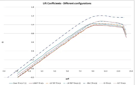
Lift Coefficients
Figures 32 to 35 show the Cl- curves for the Clean Configuration plotted together with the Xfoil Simulations. The experimental values are plotted in two ways: Cl vs. the geometrical angle of attack αgeo and Cl vs. the effective (corrected) angle of attack αeff. The measured lift approximates
to Xfoil predictions when plotted against effective angle of attack, in particular in the region where the Cl- curve is linear. A shift of approximately one degree to the right is found when compared with simulations. Furthermore, stall starts earlier in the wind tunnel (αeff ~ 9.1°) than in
NLR-TR-2014-310
|
35
The balance measurements were realized several times and presented good repeatability. Figure 36 shows six different measurements for the clean configuration at 70 m/s, where F stands for Forward (increasing AoA) and R stands for Reward (decreasing AoA), indicating which direction the balance was being turned. No hysteresis effect was found. The only case that measurements presented some difference was in the stall region for the US-TOP, when comparing two different measurements days. Because of this, two curves for the US-TOP are presented in the general comparison amid all configurations (Figure 37 and 39).
Figure 37 shows the balance measurements for all configurations (section 5.3), with exception of the FS. In the first figure, the Cl values were normalized taking into account also the area provided by the serration. Neglecting the small angle of 2.1° between the serration and the chord line, the new surface area, projected on the plane z =0, becomes
𝐴𝑠𝑢𝑟𝑓𝑎𝑐𝑒= 𝐴𝑎𝑖𝑟𝑓𝑜𝑖𝑙+ 𝐴𝑠𝑒𝑟𝑟𝑎𝑡𝑖𝑜𝑛
𝐴𝑠𝑢𝑟𝑓𝑎𝑐𝑒= (𝑏 × 𝑐) + (½ × 𝑏 × 𝑙𝑠𝑒𝑟𝑟𝑎𝑡𝑖𝑜𝑛)
where b is the span and l the length of the serration. And because 𝑙𝑠𝑒𝑟𝑟𝑎𝑡𝑖𝑜𝑛= 0.2𝑐:
𝐴𝑠𝑢𝑟𝑓𝑎𝑐𝑒= 𝑏 × 1.1𝑐 (32)
This is equivalent to say that a new chord 10% higher is being used. For the SCP, however, because of the extra 3.6 mm plate 𝑙𝑆𝐶𝑃= 0.224𝑐 and 𝐴𝑆𝐶𝑃= 𝑏 × 1.112𝑐.
Figure 38 shows the Cl-α curve with Cl values normalized with the airfoil chord only. In both
Figures 37 and 38, the measured Cl-α curves in the linear region (before stall) are parallel to each other, with a slightly difference in slope compared to the Xfoil curve. Also in the linear region, independently of the normalization method, the Cl is highest for the clean configuration, followed by (in order) SCP, CS, US-TOP, US-TOP (2) and US-BOT. Also interesting to note is that the stall region starts later for the serrated configurations, with a maximum lift around αeff ~
10.3°, while it was αeff ~ 9.1° for the clean configuration. Finally the biggest difference between
both normalization methods is that if the first one is considered (Figure 37), then the clean configuration has a higher maximum lift than all the serrated configuration, while for the second method (Figure 38) the serrations have comparable maximum lift coefficients, with SCP and
36
|
NLR-TR-2014-310because the drag is not sufficiently accurate measured by the balance, due to the precision of the
machine, the drag coefficient must be deduced from the momentum deficit in the far wake.
8.2
Hot-wire
This section presents the results obtained for the Hot-wire measurements for the Boundary Layer (4.2.1) and for the Wake (4.2.2).
Boundary-Layer
8.2.1
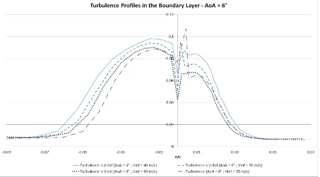
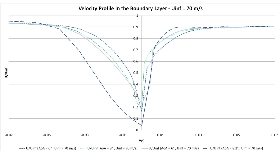
Figures 39 to 42 show a comparison among the velocity profiles in the Boundary Layer of different free stream velocities and Figures 43 to 46 compare the turbulence profiles. The pressure side is represented by the positive part of n/c (normal coordinates to the camber line over chord length), while the suction side is represented by the negative axis.
For αeff = 0° (Figure 39) the profiles are similar, not varying much with velocity. Figure 43 shows
the turbulence graphs for the same angle. The turbulence intensity is lower and returns to free stream levels faster for higher 𝑈∞, that is, in a smaller transverse distance. Hence, the boundary layer is thinner for higher 𝑈∞.
For αeff = 3° (Figure 40), at lower 𝑈∞ the velocity profiles are less full and takes longer in the transverse direction to reach the edge velocity. This also indicates bigger boundary layer thicknesses for lower 𝑈∞. Figure 44 shows the turbulence once again returning faster to free stream levels for higher 𝑈∞.
For αeff = 6° (Figure 41) again the velocity profiles are fuller for higher 𝑈∞. However, in the pressure side an exception to this trend occured, in which the 70 m/s velocity profile is the least full. This difference also is noted in the turbulence intensity graph (Figure 45), where the 70 m/s turbulence profile takes to return to free stream levels than the 60 m/s profile.
For αeff = 8.2° (Figure 42), the deficit in velocity for 60 m/s and 70 m/s are more intense in the