Tube mill optimization at Tata Steel
Tubes
Kevin R. Commandeur
B.Sc. Thesis
July 2018
Supervisors: prof. dr. ir. J. Van Hillegersberg
dr. ir. J.M.J. Schutten
Faculty of Behavioural Management and Social Sciences. Department Industrial Engineering and Business Information Systems
University of Twente P.O. Box 217 7500 AE Enschede The Netherlands
Faculty of BMS
Committee:
1st supervisor External supervisor
prof. dr. ir. J. Van Hillegersberg Sanne Kramer
Faculty: BMS Site manager
Department: IEBIS Tata Steel Tubes
2nd supervisor
dr. ir. J.M.J. Schutten Faculty: BMS
Department: IEBIS
Preface
September 2015, I attended the Kick-In introduction week at the University of Twente as a
freshman. Now, at the end of my third academic year, I am writing this preface. I realise that I have
almost finished my bachelor’s degree, which is amazing. I remember the orientation day of Industrial
Engineering and the lecturer was talking about the graduation at the end of the bachelors. It seemed so far away. In my third academic year, I went to Jyväskylä (Finland) to study abroad at the
Jyväskylän ylipisto. I followed some totally un-IEM-related courses in Finland; politics and
communication. It was a great adventure and a change of perspective. I am looking forward to the future.
First, I would like to thank Sanne Kramer, who was my supervisor at Tata Steel tubes. You gave me a lot of freedom and space to create my own ‘project’, but provided guidance when necessary. Also, I really liked our talks about people management, organizational issues and strategic planning with all the practical examples from the Tata Steel organization.
Second, I would like to thank Jos van Hillegersberg, who was my first supervisor at the University of Twente. I would like to thank you for your time, your guidance and support. We discussed many research related topic and you advised me on all the issues I encountered during the project. Third, I would like to thank Marco Schutten. Thank you for making time to be the second supervisor of my thesis.
I wish Sanne, Jos and Marco all the best in the upcoming future in both their personal and professional lives.
Management summary
The aim of the research was to alter the processing speed of the bottleneck in the M-93 (tube mill at Tata Steel Tubes). Increasing the processing speed of the bottleneck implies that the speed at which the tubes arrive in the outside storage increases and since the demand of the tubes in the research scope is higher than the supply, an increased speed implies an increased turnover and profit. The
goal was set to increasing the bottleneck’s processing speed up to the speed of the tube mill, since the bottleneck is stalling the tube mill massively. The research scope was set to the tubes that are bundled with 2 tubes in one bundle, which are the 323 and 273 (tube diameter). These numbers will be used to refer to the tubes with the corresponding diameter.
We conducted literature research to set up a theoretical framework to support the reasoning and decisions in the field research. The topic of the theoretical framework is the Theory of Constraints (TOC). In the field research, several TOC tools, TOC methodology, TOC definitions and TOC logic is used to form arguments and describe phenomena. The first step in the field research was to identify the constraining process of the production line. This turned out to be the bundling process. We distinguish two processes in the bundling process:
1. Forming the desired bundle shape: how many tubes per bundle and how are they stacked upon each other?
2. Strapping the bundle.
The second step turned out to be the bottleneck. We took time samples from the strapping process and set up a timeline of the process. Additionally, we analysed the strapping process with the use of a Current Reality Tree (CRT). The combination of the timeline and the CRT provided a clear picture of the current situation and has set the direction of the solution generation phase. The process
downstream of the strapping process, which is the placement of the previously strapped bundle in the draining queue, turned out to be stalling the strapping process. This is the most prominent constraining factor of the strapping process. Reducing the processing time of placing the previously strapped bundle in the draining queue will decrease the time that the strapping process is hindered. Furthermore, with the use of 3 Evaporation Clouds (a TOC tool), 3 additional improvement
possibilities have been identified:
1. Invest in an additional strapping machine to increase capacity
2. Strap with a stronger strapping material to reduce the number of straps needed from 6 to 4. 3. Increase the number of tubes in one bundle from 2 to 5 tubes.
We determined the effectiveness of reducing the processing time of placing the previously strapped bundle and the 3 additional improvement possibilities with the use of a simulation study. A decrease in processing time of 25% of placing the previously strapped bundle in the draining queue, would increase the strapping speed with approximately 17%. Furthermore, combining this intervention with an extra strapping machine or stronger strapping material increases the strapping speed with approximately 40%. Finally, increasing the tubes per bundle from 2 tubes to 5 tubes will increase the strapping speed to 70.6 meter per minute, however this intervention can only be implemented for the 323 and 273 with a wall thickness up to 5 mm and only a part of the customers can process bundles of 5 tubes.
Based on the research we recommend taking the following steps:
1. Identify customers that can process bundles of 5 tubes for the 323 and 273 with a wall thickness up to 5 mm. Supply those customers, the bundles consisting of 5 tubes.
3. Decrease the time that the strapping process is hindered by placing the previously strapped bundle in the draining queue.
4. Switch from the 31.75x0.8 MK strapping material to the 31.75x0.8 HT strapping material, which has a higher break force. This will result in a reduced strapping time and reduces the number of straps needed to strap one bundle. Further research is required to determine the effect of the increased strap strength on the tubes outside of this research scope.
The goal has been met for a part of the tubes in the research scope. After the recommended
interventions for 55% of the tubes in the research scope, the strapping speed is higher than the tube
mill’s speed and for 85% of the tubes the difference between tube mill speed and strapping speed is only 6.5 meter per minute or lower. Figure 1 shows the distribution of the difference between tube mill speed and strapping speed in the current reality and future reality. Future reality refers to the scenario after the recommended interventions have been implemented. The centre of mass in the current reality is mostly focussed on the right side of the graph, which implies a big difference between tube mill speed and strapping speed. In the future reality, the centre of mass has moved to the left side, which implies a very low difference or non-existing difference between the tube mill speed and strapping speed.
Figure 1: Distribution of the difference between the tube mill speed and strapping speed
0% 10% 20% 30% 40% 50% 60%
<0 <0, 6.5> < 6.5, 13> <13,19.5> >19.5
FR
A
CT
IO
N
O
F T
H
E
TUBE
S
IN
R
ES
EA
R
CH
S
CO
PE
DIFFERENCE BETWEEN TUBE MILL'S SPEED AND STRAPPING SPEED = TUBE MILL SPEED - STRAPPING SPEED
Distribution of the difference between tube mill speed and strapping
speed
Contents
1 Definitions ... 1
2 Introduction ... 3
2.1 Intro to Tata Steel Tubes ... 3
2.2 The problem ... 3
2.3 The problem-solving approach ... 3
2.4 Research ... 3
2.5 Report outline ... 4
3 Theoretical framework ... 5
3.1 Optimal process optimization methodology ... 5
3.2 The TOC methodology ... 6
3.3 TOC measurement ... 6
3.4 Drum-Buffer-Rope principle... 7
3.5 TOC application: Drum-Buffer-Rope ... 8
3.6 TOC application: the thinking processes ... 9
3.6.1 Current reality tree ... 10
3.6.2 Evaporating cloud ... 11
3.6.3 Future reality tree ... 11
3.6.4 Prerequisite tree ... 11
3.6.5 Transition tree ... 12
3.6.6 Conclusion literature review ... 12
4 Production line analysis ... 13
4.1 Process description of the M-93 ... 13
4.2 Data gathering: processing speed ... 14
4.2.1 Tube mill ... 14
4.2.2 Bundling process ... 15
4.2.3 Draining process ... 15
4.2.4 Transportation process ... 16
4.2.5 Processing speed analysis ... 17
4.3 Deep-dive research into the bundling process ... 18
4.4 Current Reality Tree ... 20
4.5 Intermediate conclusion: RQ1 ... 21
5 Solution generation... 23
5.1 Evaporation clouds... 23
5.2 Bottleneck: downstream process hinders strapping ... 23
5.4 Additional improvement possibility 2 ... 26
5.5 Additional improvement possibility 3 ... 26
5.6 Future Reality Tree (FRT) ... 28
6 Simulation study ... 29
6.1 The model in general ... 29
6.2 Input: ... 30
6.3 Output: ... 30
6.4 Assumptions ... 30
6.5 Simplifications ... 31
6.6 Technical details of the model ... 32
6.7 Model Verification ... 34
6.8 Model validation ... 34
6.9 Output verification & analysis... 34
6.9.1 Differing experiment setups & the same output: ... 36
6.9.2 Cross-case analysis ... 36
6.10 Intermediate conclusion: answer to RQ2 ... 37
7 Investments ... 38
8 Conclusion ... 39
9 Discussion ... 40
10 Bibliography ... 42
11 Appendix ... 44
11.1 Appendix A ... 44
11.2 Appendix B ... 44
11.3 Appendix C ... 45
11.4 Appendix D ... 45
11.5 Appendix E ... 46
11.6 Appendix F ... 49
11.7 Appendix G ... 53
11.8 Appendix H ... 53 12 Reflection ... Error! Bookmark not defined.
1
1
Definitions
General definitions
TOC: Theory of constraints
KPI: Key performance indictor
WIP: Work in progress
Chain: The chain of processes
Workstation: One of the processes in the chain
Tube profile: The shape of the tube, which can be round, rectangular or squared.
ROI: Return on investment
Net profit: Profit minus all operating expenses
Cash flow: Cash and cash-equivalents moving into and out of a business
Downstream: All the workstations after the workstation in question
Upstream: All the workstations before the workstation in question
Plant Simulation: The software program that is used to simulate the M-93
Processing time: The time it takes for a workstation to produce 1 product
OEE: Overall equipment effectiveness, which is determined by quality, speed and availability.
In-line measurement data: measurements taken in the tube mill while producing tubes. TOC definitions
The system: The whole chain of processes that start when an order is received and ends when the order has been paid for.
The bottleneck: the process which capacity equals or is below the demand (Goldratt, 1999)
Throughput rate: The rate at which the system generates money through sales (Naor & Coman, 2013), (Tulasi & Rao, 2012)
Inventory: All the money that the system invests in purchasing things it intends to sell (Naor & Coman, 2013), (Tulasi & Rao, 2012)
Operations expenses: All the money the system spends to turn inventory into money (Naor & Coman, 2013), (Tulasi & Rao, 2012)
DBR: Drum-Buffer-Rope concept
Thinking Processes (TP): Logic diagrams that are used identify the constraint and increase its performance
Current Reality Tree (CRT): One of the TP tools, for more info see the section on TP
Evaporating Cloud (EC): One of the TP tools, for more info see the section on TP
Future Reality Tree (FRT): One of the TP tools, for more info see the section on TP
Prerequisite Tree (PT): One of the TP tools, for more info see the section on TP
Transition Tree (TP): One of the TP tools, for more info see the section on TP
UDEs: Undesired effects
3
2
Introduction
2.1
Intro to Tata Steel Tubes
Tata Steel Tubes is a subsidiary of Tata Steel Europe. Tata Steel Tubes has 3 sites in the Netherlands: one in Zwijndrecht, one in Oosterhout and one in Maastricht. All these sites are located near rivers to ensure a constant supply of steel from Tata Steel IJmuiden. This research has been conducted at the production site in Zwijndrecht and focussed on the tube mill called the M-93. The tubes
produced at the M-93 are used in the construction industry. In this report M-93 refers to the whole chain of processes from tube mill to the outside storage.
2.2
The problem
The speed at which the 323 and 273 (tube diameter in mm) arrive in the outside storage is too low. Currently, the processing speed of the tube mill is far higher than the speed at which the tubes arrive in the storage. This indicates that the output speed is constrained by one of the processes between the tube mill and the outside storage. This constraining factor leads to the tube mill being
stalled, which implies that the tube mill’s capacity is lost. The goal of this graduation project is to find an interventention that can alter the processing speed of the bottleneck up to the processing speed of the tube mill. The exact bottleneck still has to be pinpointed. Furthermore, the demand of the 323 and 273 is bigger than the current supply, so an increase in output speed implies an increase in sales. The processing speed of the tube mill differs depending on the wall thickness, diameter and length of the tube. The research scope consists of the 273 and 323. The total product range, concerning wall thickness is included and the tube length equals 12 meters. The tube length has been set to 12 meters, because that is the most common tube length that is produced. Appendix A shows the processing speed of the tube mill when producing the tubes in the research scope (norm values).
2.3
The problem-solving approach
First, we conducted a literature review on production process optimization theory. Second, we performed an in-depth analysis of the production line to find the cause for the underperformance on the output speed. The research variable ‘processing speed per workstation’ in combination with a current reality tree were used to find the cause. We found appropriate solutions after implementing the evaporation cloud and future reality tree (Theory of Constraints). Finally, we determined the effectiveness of the solutions with the use of a simulation study.
2.4
Research
The research is guided by the following questions:
(1) What is the cause of the underperformance on the speed at which the tubes arrive in the outside storage of the M-93 at Tata Steel Tubes?
Goal: To identify the bottleneck and to understand the cause of the problem, such that the proposed interventions address the problem accurately.
(2) What interventions can eliminate the cause of the underperformance on the speed at which the tubes arrive in the outside storage of the M-93 at Tata Steel Tubes?
Goal: To find effective solutions to the problem.
Sub1-RQ1: What is the processing speed of the tube mill, bundling process, draining process and transportation process to the outside storage in meters of tube per minute?
Goal: To find the bottleneck workstation, after which it can be analysed in detail to find the root cause.
Sub2-RQ2: How to apply the Theory of Constraints to (1) identify the constraint and (2)
increase the constraint’s capacity?
4 The sub-research questions were used to answer the main questions 1 and 2.
2.5
Report outline
5
3
Theoretical framework
The theoretical framework answers the question: How to apply TOC to (1) identify the constraint and (2) increase the constraint’s capacity? Before TOC has been chosen as a theoretical framework,
a preliminary literature review has been conducted on different process optimization theories. This preliminary research will be explained in 2.1. The main part (starting from 2.2) consists of two parts. The first part consists of an introduction on TOC. It’s problem solving methodology, TOC
measurement, the reasoning behind TOC and the Drum-Buffer-Rope principle (DBR) will be
explained. The second part will go into the application of TOC, so the thinking processes (TOC tools) and the application of DBR are described.
Note: Some of the terms used below are defined differently compared to their definition in other scientific literature. The definitions can be found in 1. definitions –‘TOC definitions’.
3.1
Optimal process optimization methodology
We compared the Theory of Constraints (TOC), Lean and Six Sigma to find the best fitting process optimization methodology to address the problem at Tata Steel Tubes. This paragraph describes the differences between the three. The focus of the three methodologies differ. TOC focusses on the bottleneck in the chain to increase the chain’s throughput, Lean focusses on the reduction of waste
in the whole chain and Six Sigma focusses on the reduction of variance (Nave, 2002). The effect of a reduced variance in the chain because of Six Sigma is a more uniform and reliable output. The reduced waste (Lean) leads to decreased costs and reduced flow time. The Six Sigma approach relies heavily on measurement, data and statistical analysis. Unfortunately, Tata Steel Tubes does not have the measures to perform such an advanced analysis concerning the problem at hand. The big
difference between TOC and Lean is that Lean has a ‘whole chain’ approach and TOC takes a ‘bottleneck‘ approach (Dettmer, 2008). Since, reduced waste is the desired effect of Lean, it is best
to analyse the whole chain and remove all the identified waste. The purpose will be achieved. However, this is not the best way to increase the throughput. The throughput is determined by the processing speed of the bottleneck, thus reducing waste in non-bottleneck processes will not increase the throughput. In the first phase of TOC, the bottleneck is identified and the next four steps focusses explicitly on the bottleneck. The methodologies have secondary effects, for example the reduced variance (Six Sigma) will increase throughput and the reduced waste (Lean) will decrease flow time and increase throughput, but the methodologies have the biggest impact on their primary focus. The focus of the study is to increase the output speed of the whole chain. Currently, the output speed is lower than the tube mill’s speed. This implies that the output speed is constrained by one of the processes between the tube mill and the outside storage. The focus of the study should be in line with the focus of the optimization methodology. TOC meets this criterium most accurately.
Some scholars criticize TOC. They argue that the TOC results are feasible, but not optimal (Watson, Blackstone, Gardiner, 2006). However, Mabin (2003) conducted a study on the success of TOC. She conducted a meta-analysis of 80 TOC applications. All the TOC applications showed significant improvements in both operational and financial performance. Despite, extensive searches, the research found no reports of failures (Mabin, 2003). Noar, Bernardes and Coman (2012) evaluated
the Theory of Constraints on whether it is a valid theory of not. They used Wacker’s framework for theory building for the evaluation. Wacker’s framework was used, because it reflects apparent
6
3.2
The TOC methodology
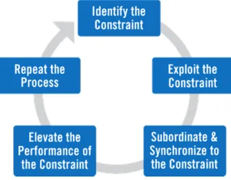
Eliyahu M. Goldratt is the originator of the Theory of Constraints (Goldratt, 2004). The TOC philosophy focusses on continuous improvement of a certain system. The theory has been applied by many companies with tremendous success (Mabin, 2003). A major component of TOC that underpins all the other parts of the methodology is the TOC Thinking Processes. They address the 3-fundamental questions of (1) What to change? (2) What to change it into? (3) How to cause the change? They guide the user of the TOC methodology through the decision-making process of the problem structuring, problem identification, solution building, identification of barriers to be overcome and implementation of the solution.
TOC views the system as a chain and each process in the chain as a link. All the links need to work together to achieve the goal of the chain. In the TOC literature the chain is called ‘The system’. It is assumed that there always is 1 constraining factor that limits the performance level of the chain. The theory of constraints does not view this constraining factor in a negative way, but to the contrary in a positive way. The constraining factor is the key to optimization. If the constraining factor is identified, it can be acted upon or the other operations can be set to operate with it. The TOC methodology follows the following steps:
(1) Identify the constraint in the system.
(2) Exploit the constraint. Exploiting the constraint implies that the constraint performs at its 100% capacity.
(3) Subordinate the other processes in the system to the constraint. The performance of the other processes should meet the performance of the constraint to prevent excessive inventory and high operation expenses.
(4) Elevate the performance of the constraint and by doing so, elevate the performance of the system.
(5) Repeat the process
Mabin (2018) and
Ş
imşit et al. (2014) argue that TOC does not contain 5,but 7 steps. The two additional steps need to be performed before the 5 aforementioned steps. The two additional steps are: (1) Determine the goal of the system (2) Set up measures of the system. If the goal and measures are defined, the 5 steps above can be executed.
3.3
TOC measurement
TOC argues that, in the end, the goal of each company is to earn as much profit as possible. If this is
not the company’s ultimate goal, it is certainly a critical success factor (Dettmer, 2008). This implies that the output of the system must be money and that the system must be designed in such a way that it generates the highest profit possible. The goal of generating the highest amount of money can be translated to a high net profit, a high Return on Investment (ROI) and a high cash flow. We have introduced measurable terms for the goal, but these measures are calculated at the end of the whole process, so we lack the measures that represent how well the system is performing in terms of its goals during operation time. Goldratt (1999) introduced throughput rate, inventory and operating expenses to be able to measure the performance of any system during operations hours. Those terms are defined differently compared to their definitions in most of the scientific literature (1. Definitions)
If those KPIs represent the goal, there must be a relationship between the net profit, ROI and the throughput rate, inventory and operational expenses. The net profit (1) is expressed as the
[image:13.595.402.569.306.436.2]difference between the throughput rate and the operational expenses, ROI (2) equals the division of the difference between throughput rate and operating expenses by inventory and cash flow equals
7 net profit divided by the increase or decrease of inventory (Naor & Coman, 2013), (Tulasi & Rao, 2012).
(1) 𝑁𝑒𝑡 𝑝𝑟𝑜𝑓𝑖𝑡 = 𝑇ℎ𝑟𝑜𝑢𝑔ℎ𝑝𝑢𝑡 𝑟𝑎𝑡𝑒 − 𝑜𝑝𝑒𝑟𝑎𝑡𝑖𝑜𝑛 𝑒𝑥𝑝𝑒𝑛𝑠𝑒𝑠
(2) 𝑅𝑂𝐼 =𝑁𝑒𝑡 𝑝𝑟𝑜𝑓𝑖𝑡𝐼𝑛𝑣𝑒𝑛𝑡𝑜𝑟𝑦= 𝑇ℎ𝑟𝑜𝑢𝑔ℎ𝑝𝑢𝑡 𝑟𝑎𝑡𝑒−𝑜𝑝𝑒𝑟𝑎𝑡𝑖𝑜𝑛 𝑒𝑥𝑝𝑒𝑛𝑠𝑒𝑠𝐼𝑛𝑣𝑒𝑛𝑡𝑜𝑟𝑦
(3) 𝐶𝑎𝑠ℎ 𝑓𝑙𝑜𝑤 = 𝑇ℎ𝑟𝑜𝑢𝑔ℎ𝑝𝑢𝑡 𝑟𝑎𝑡𝑒−𝑜𝑝𝑒𝑟𝑎𝑡𝑖𝑜𝑛 𝑒𝑥𝑝𝑒𝑛𝑠𝑒𝑠∆ 𝐼𝑛𝑣𝑒𝑛𝑡𝑜𝑟𝑦
*The operation expenses and inventory should be measured over the same time period as the throughput rate *All the variables are expressed in the same units (1. Definitions)
The formulas above show the relationship between the KPIs and the goal. To achieve a high net profit, the throughput rate should be as high as possible and the operating expenses should be as low as possible. To achieve a high ROI, the throughput rate should be as high as possible and the operation expenses and inventory should be as low as possible. To achieve a high cash flow, the throughput rate should be as high as possible and the operation expenses and inventory as low as possible (Tulasi & Rao, 2012). To conclude: the aim of a company is to increase the throughput rate, while decreasing the inventory and operation expenses (figure 3).
Figure 3: Relationship between earning profit and through put, operations expenses and inventory
3.4
Drum-Buffer-Rope principle
The Drum-Buffer-Rope (DBR) principle ensures that the bottleneck is exploited and the other processes in the system are subordinated to the bottleneck. There are two important factors that
affect the system’s performance. The first factor is the relation between statistical fluctuation and dependent events and the second factor is the utilization of the workstation capacity of the different workstations in a production line. DBR, takes those factors into account and minimizes their negative effect on the throughput, inventory and operations expenses. An explanation of the two factors is presented below.
Imagine a production line with 5 workstations. Each workstation can start its process, if the
workstation before the workstation in question provides the workstation with input or if there still is remaining input in the buffer. This implies that if the output of workstation 1 + the buffer prior to workstation 2 does not meet the potential capacity of workstation 2 at that moment, that the capacity of workstation 2 will not be fully utilized for that time period. Strategically placed buffers can prevent this from happening. On the other hand, buffers are additional costs, so a trade-off between the costs of the buffer and its positive effect on the output should be made.
8 Figure 4 presents a visualization of a production line that will support the explanation of the effect of statistical fluctuation and dependent events. The workstations do not have buffers. The numbers in the circles represent the interval of the output per hour of each workstation, so the output varies between 3 and 5 per hour. The average output will be 3+52 = 4. Instinctively, most people would argue that this production line will produce 24 × 4 = 96 products per day (assuming a uniform distribution). This is not the case, due to statistical fluctuation and dependent events. Dependent events are events that can only start, if another event has finished. In the production line, each process in the chain is a dependent event of the process prior to the process itself. Furthermore, each workstation shows statistical fluctuation in its output, so with a certain probability the output varies between 3 and 5. The output of the whole chain equals the output the workstation with the lowest output in the chain. This implies that if one of the 5 workstations in the chain has an output of 3, the output of the chain will equal 3 and if and only if, all the workstations in the chain have an output of 5, the output of the chain equals 5. The probability that one of the workstations will have an output below average is higher than the probability that all the workstations will have an output above average, therefore the output of the chain will be below the suggested 4 products per hour. However, if strategic buffers were added to this production line, the negative effect of the statistical fluctuation on the output can be absorbed. More on the buffers 2.5.
The second factor is the utilization of the workstation capacity of the different workstations in the production line.
Figure 5: Visualization of a production line (numbers represent maximum capacity)
In the visualization of a production line in figure 5, the circles represent workstations and the numbers in the circles represent maximum capacity per hour and therefore the workstation’s
maximum output per hour. It seems intuitively that working hard will achieve the goal, however if the workstations in the production line above will work at their 100% capacity Work in Progress (WIP) will accumulate in front of the workstation with maximum capacity 8 and 5, since the input of those workstations is higher than their output. This implies that output of the whole chain is set by the workstation with the lowest capacity. In terms of TOC, inventory and operation expenses are unnecessary high. Inventory is high, because the amount of money spend on intermediate goods in the production line rises and the operation expenses are high, because the workforce of the
workstation with maximum capacity 10, 9 and 8 are working harder than required, since the output of the chain will not increase if those workstations have an output above 5. Subordination of the output of those workstations to the output of the workstation with the lowest output will minimize inventory and operation expenses.
3.5
TOC application: Drum-Buffer-Rope
The statistical fluctuation in combination with dependent events and capacity utilization are important factors that influence the output of the production line. It is important to protect the system against the effect of the relation between statistical fluctuation and dependent events and to subordinate the utilization of the workstations to the capacity of the bottleneck. Drum-buffer-rope is TOC production principle that takes those factors into account. It is named after the 3 core
9 that protects the drum from statistical fluctuation upstream in the production line. The rope is symbolic for the timing of the release of products by the workstations upstream of the drum. The drum-buffer-rope application starts with an already identified bottleneck. The bottleneck is the drum, which sets the pace of all the other workstations in the system. Since the bottleneck
determines the output of the whole system, the bottleneck should always work on its full capacity to achieve maximum output of the system. In other words: “the bottleneck should be exploited”.
Exploitation of the drum is achieved with the use of a time-buffer. The buffer is the time interval that predates the release of work relative to the date on which the constraint will process the work. This differs from the more common perception of a buffer, which is measured in terms of physical goods. The time buffer in the TOC will, however, result in an accumulation of physical goods in front of the bottleneck for a large percentage of the operating time of the system. This accumulation protects the drum from statistical fluctuation upstream of the production line. When determining the length of the time buffer, the statistical fluctuations should be considered. This implies that the buffer should be longer than the sum of the waiting time in the queue + the average processing time of all the workstations upstream + the variance of the processing time of all the workstations upstream. This is a very simplified description of how to determine the buffer length. Ye and Han (2008) have developed mathematical models to determine the buffer length. The time buffer ensures that the bottleneck will always be working.
We protected the drum, now it is time to protect the system by subordinating all the workstations to the drum. Subordination of the processes to the drum is key to inventory reduction. The buffer must
be stable; thus, the system’s input must equal the drum’s output. If the bottleneck is not working for
a period of time, this must be reflected in the system’s input, otherwise the WIP will increase each time the bottleneck is in down-time. This is the job of the constraint rope. The constraint rope can be seen as a real-time feedback loop between the drum and input of the system. The constraint rope coordinates the input of the system with the output of the drum.
Until now we have discussed the part upstream of the bottleneck. Now it is time to discuss the part downstream of the bottleneck. The output of the system must be on time. To ensure that the output is on time, we introduce the shipping buffer. The shipping buffer is the time interval that predates the release of work relative to the date on which the product should be shipped. The definition is the same as with the bottleneck buffer, but it covers a different part of the system. Again, to prevent accumulation of inventory, we will need a mechanism that relates the market demand with the drum. This mechanism is the shipping rope and it works according to the same principles as the constraint rope.
3.6
TOC application: the thinking processes
The Thinking Processes (TPs) tools are a set of logic diagrams that are used to answer the
3-fundamental questions in TOC: (1) What to change? (2) What to change to? (3) How to change? The TPs can be used individually or in combination. The TPs consists of five logic diagrams:
(1) Current Reality Tree (CRT) (2) Future Reality Tree (FRT) (3) Prerequisite Tree (PT) (4) Transition Tree (TT)
(5) Evaporating Cloud (EC), also referred to as the Conflict Resolving Diagram (CRD)
The CRT, FRT and TT are build up by constructing connections between observed effects and their
causes based on ‘sufficient cause’. A cause is a sufficient cause if the cause inevitably leads to a
certain consequence. An example: ‘if it rains, the earth gets wet’. In this case, the rain is a sufficient
10 necessary of condition B if condition A is necessary to achieve condition B. An example: a bike (A) is necessary to cycle to school (B).
The problem analysis in the TOC methodology is based on the assumption that undesired effects exist because of a few number of root causes. The TPs identify those root causes and offer solutions to eliminate them. (Librelato & Lacerda & Rodrigues, 2013). The purposes of the individual TPs and the relationship between the fundamental question and the TPs are presented in figure 6.
Figure 6: Relationship between TPs and the 3 fundamental questions in TOC
(Librelato & Lacerda & Rodrigues, 2013)
3.6.1
Current reality tree
The current reality tree is a logic diagram that is used to find the root-cause of a problem. The CRT is based on cause-effect logic. It aims to identify the cause that is responsible for most of the
Undesired Effects (UDEs). By focussing on that particular cause, we can address multiple UDEs at the same time. The use of the CRT will help to identify physical as well as non-physical constraints. Setting up a CRT starts with identifying all the undesirable effects (UDEs). The next step is to examine the cause-effect relations between the UDEs. The easiest way to do this is to set the UDE that does not cause an other UDE at the top of the CRT and work downwards to find the root-cause of the UDEs in the CRT. When examining the relationships between the UDEs it is important to distinguish between the following cause-effect relations (Scoggin &
Segelhorst & Reid, 2003):
• 1 UDE can be the cause for multiple UDEs
• multiple UDEs, together, are the cause of one UDE
• 1 UDE can be the cause for another UDE In the graphical representation of the hypothetical CRT (figure 7) ellipses represent an ‘AND’ relation, which means that the causes, together, result in the effect. Neutral effects are effects that are, on itself, neither positive nor negative, but cause a UDE. Neutral effects can be added to create a better representation of reality in the CRT (Based on: Scoggin & Segelhorst & Reid, 2003) (Based on: Umble & Murakami, 2006).
11
3.6.2
Evaporating cloud
The Evaporating Cloud (EC) or the Conflict Resolving Diagram (CRD) is used to ‘evaporate’ or ‘resolve’ a conflict between ideas or opinions. A conflict can exist in many scenarios; therefore, the EC can be used in many situations. The EC consists of ‘wants’, ‘needs’ and an‘objective’. The
conflicting ‘wants’ of two people, are the result of their ‘needs’ and those needs should be in line with a common objective.
The CRT has been used to identify the core problem that needs to be addressed. In most of the cases the core problem is caused by two conflicting ‘wants’ of two people. TOC offers the evaporating cloud to resolve this conflict and turn it into a desirable solution for all the parties involved. The EC is based on the assumption that conflicts are the result of believing an incorrect assumption, therefore conflicts can be solved by correcting the incorrect assumption. The EC helps to do so. It examines the logic behind the conflict and its underlying assumptions. (Based on: Chaudhari & Mukhopadhyay, 2003)
Setting up the EC starts with the two conflicting ‘wants’. The two conflicting ‘wants’ are a result of the two conflicting ‘needs’. The needs are necessary to meet a certain objective. I want D, because I need B/C to meet A (figure 8).
The next step is to add the assumptions on which the relationships (denoted by the arrows) are based. One of the assumptions will be incorrect and therefore the initially seeming logical
relationship will not be so logical anymore and the conflict will be resolved. Finding the incorrect assumption will help to find an injection (solution). The evaporating cloud ensures that the user thinks critically of all the components in the conflict and challenges the assumptions that are made.
3.6.3
Future reality tree
The Future Reality Tree (FRT) is used to examine the
effectiveness of the solution that has been found with the use of the EC. Basically the injection (solution) that comes out of Evaporation Cloud is added to the CRT. The logic behind the FRT is that, the moment that the injection is inserted in the CRT, UDEs should turn into Desirable Effects (DEs) based on valid cause-effect logic. By doing so, the FRT serves as a tool to evaluate the effectiveness of the injection. (Based on: Scoggin & Segelhorst & Reid, 2003)
3.6.4
Prerequisite tree
The aim of the Prerequisite Tree (PT) is to set up the goals of the implementation plan of the
solution. It allows us to overcome the obstacles that stop us from implementing our plan. Setting up the Prerequisite Tree starts with the injection that came out of the analysis of the EC. Each injection requires its own PT. The next step is to determine the obstacles that hinder us from implementing the injection and by determining the obstacles we can simultaneously determine the intermediate objectives. The last step is to decide the order in which the intermediate objectives should be met, which is the same as deciding on the order in which the obstacles should be overcome. This order is set by necessity logic: intermediate objective A should be met before objective Q can be met.
12
3.6.5
Transition tree
The transition tree is a tool that sets the actual implementation plan. It connects the intermediate goals to actions based on if-then logic and sets the order in which the intermediate objectives should be met. It also adds a reason on why the action will result in meeting the demand. (Based on: Scoggin & Segelhorst & Reid, 2003)
3.6.6
Conclusion literature review
Sub2-RQ2: How to apply the Theory of Constraints to (1) identify the
constraint and (2) increase the constraint’s capacity?
The Theory of Constraints offers a framework for continuous improvement.
The process starts with a goal and measurement. The end-goal of each company is to earn money. In the production scene, this goal can be measured by measuring throughput, operation expenses and inventory. When the goal and the measurement is set, the bottleneck of the system must be identified. Second, the bottleneck should be exploited. Third, the other processes should be
subordinated to the bottleneck. The fourth step is to elevate the constraint. The identification of the bottleneck can be conducted by an analysis of the measure ‘throughput’ in combination with a Current Reality Tree. The subordination and exploitation phase can be executed through the application of the Drum-Buffer-Rope principle. The evaporation cloud can be used to determine the appropriate injection (solution) to address the problem in the elevation phase. The future reality tree provides a check-up of the effectiveness of the injection based on cause-effect logic. Lastly, the prerequisite tree identifies the obstacles and intermediate objectives for the implementation of the injection and the transition tree draws up the implementation plan.
13
4
Production line analysis
4.1
Process description of the M-93
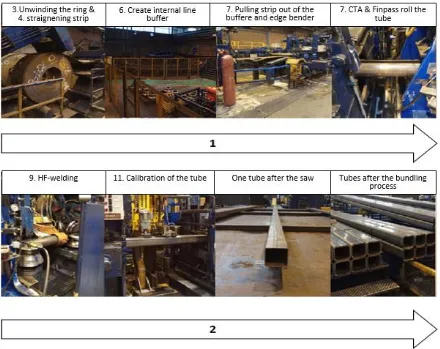
The steps below present the process of the M-93 from coil to a bundle of tubes in the outside storage.
1. The input of the production process is a coil (1. Definitions) and the output is a bundle of tubes.
2. The coil, which is the input product, goes through the slitting machine to get the right proportions depending on the tube produced. The output of the slitting machine is a rolled up narrow strip, this intermediate good will be referred to as ‘ring’.
3. The ring gets transported to the decoiler, which unwinds the ring.
4. The narrow strip goes through the straightening machine, which straightens the narrow strip. Before the straightening machine, the narrow strip tends to bend, because it has been rolled up.
5. The MIG welder welds the previous ring of narrow strip to the new ring of narrow strip. This ensures that the tube production is a continuous process.
6. The ring gets unrolled. A buffer is created. The buffer is needed, because the MIG welding takes time and the aim of the production line is to have continuous stream output. 7. The narrow strip in the buffer gets pulled out of the buffer into the edge bender. The edge
bender bends the edges of the narrow strip. The bended edges are required for the HF welding, later in the production line.
8. The narrow strip goes through the CTA and Finpass, which roll the steel into a round profile. 9. HF welding of the tube. The two sides are welded together. A round tube is created.
10. Cooling down of the hot tube
11. The tube goes through a calibration machine. If required the machine forms the round tube into a square or rectangular one.
12. The saw makes sure the tube has the right length
13. The singular tubes with the right profile and length are bundled together with 1, 4 or 6 extra tubes
14. The tubes are drained. During the production process, the tubes are sprayed with an emulsion. This emulsion is environment unfriendly, therefore they need to be drained. 15. The tubes are transported to the outside storage.
14
4.2
Data gathering: processing speed
The research variable ‘processing speed per workstation for the tubes in the research scope in
meters of tube per minute’ has been used to identify the bottleneck. Meetings with experts on the M-93 identified potential bottleneck workstations. The potential bottlenecks are the workstations between the tubemill and the outside storage, which is obvious since the output speed is
constrained by one of the workstation between the tube mill and the outside storage as stated in the introduction. The workstations in the research population are:
• Tube mill (consisting of the CTA, Finpass, HF-welding, calibration and saw)
• Bundling process
• Draining process
• Transportation process
The tube mill is added to the research population, since the bottleneck should meet the tube mill’s
processing speed.
4.2.1
Tube mill
The maximum processing speed of the tube mill is already measured by Tata Steel Tubes. This data is presented in appendix A. The data has been validated with an interview with Eric van de Steen. The data shows 2 important patterns:
[image:21.595.87.527.77.426.2]15 2) When the diameter of the tube increases, the production speed decreases, because the
width of the narrow strip increases when the diameter of the tube increases. The increased width of the narrow strip implies that the welding torch, which welds the previous ring to the new ring, covers a longer distance, which takes more time.
4.2.2
Bundling process
The bundling process involves 3 machines: the MAIR and 2 strapping machines. The MAIR creates the shape of the bundle, by stacking the required number of tubes in the desired order. After the bundle shape is created, the tubes are strapped with several straps, depending on the tube type. The two strapping machines work simultaneously. The necessary number of straps depends on the length and weight of the tubes in the bundle. In the case of the tubes in this research scope, currently, 6 straps are necessary.
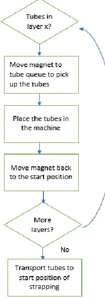
To create the shape of the bundle, the MAIR places a layer of tubes on top of another layer with the use of a magnet. In case of the first layer, the MAIR places the layer of tubes on the bottom of the machine. A layer can consist of multiple tubes depending on the diameter of the tubes, because the magnet has a fixed length. The process of the MAIR consists of the following steps:
(1) Start in the start position
(2) Move to the queue of tubes and pick up the necessary number of tubes for 1 layer
(3) Move the layer into the machine (4) Return to the start position
This cycle takes 25 seconds and is repeated until the necessary shape has been created. The tubes in research scope are bundled with 2 tubes in one bundle (24 meter of tube). The MAIR can pick up two tubes at the same time, therefore it needs to create one layer and since one layer takes 25 seconds, the MAIR has a processing speed of 24 ∗ (60
25) = 57.6 meters of tube per minute. Figure 11 shows a visualization of the process of the MAIR.
When the bundle shape is created, it is transported to the 2 strapping machines, which strap 2 straps simultaneously. 6 straps are used, so one bundle needs to pass the two machines 3 times. One cycle, that starts when the bundle is transported to the strapping machine and ends when the bundle has left the strapping machine, takes approximately 70 seconds. In those 70 seconds, the strapping machine processes 24 meters of tube, which implies a processing speed of approximately 21 meters of tube per minute.
The measures above, already existed at Tata Steel Tubes. I validated them with time-samples.
4.2.3
Draining process
[image:22.595.457.561.232.525.2]The draining process quickly drains the accumulated emulsion of two bundles by lifting one side of each bundle; the emulsion flows to the lower side. When the bundles are strapped they are moved to the queue in front of the draining process. When the second bundle enters the queue, a sensor sends a signal to the computer which lowers the draining bundles and moves those to the bundle stacking process. Simultaneously, the tubes in the draining queue move to the draining machine and the whole cycle starts all over again. The important thing to note is that, in the current reality, the draining time depends on the number of bundles in the queue; at Tata Steel Tubes it is assumed that the time it takes for 2 tubes to enter the draining queue is always bigger than the time it takes to sufficiently drain a bundle of tubes. When the bundles enter the queue at a fast pace, the draining
16 time becomes shorter, since the sensor is activated more frequently. Since the draining time is dependent on the number of bundles in the queue and therefore dependent on the speed at which the bundles arrive in the queue, the draining process cannot be a bottleneck.
4.2.4
Transportation process
The transportation process is a difficult process to analyse, because it is not an automated process and fully initiated by the Tata Steel Tubes’ workforce, which makes it prone to variability on its speed performance. The transportation process follows the following steps:
(1) An X number of bundles of tubes are stacked together and lifted on a truck. (2) The truck drives the stack of bundles to the outside storage
(3) The stack of bundles is lifted from the truck, by a forklift and placed in the outside storage. (4) The truck returns to the M-93 to pick up a new stack of bundles.
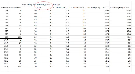
Time estimations of each step in the process are displayed in figure 12 and 13. The estimations are ranges that indicate the smallest and largest time one step in the transportation process can take. The transportation process differs between the 323 and 273 in the loading capacity of the truck. The loading capacity of the 323 is 192 meters of tube and the loading capacity of the 273 is 384 meters of tube. Furthermore, in case of the 273 it is impossible to load all the tubes at once, therefore it takes two hoists. Loading the 323 tubes only takes one hoist. ln figure 12 and 13, the red bars show the lowest time each step in the process can take and the grey bars show the longest time each step in the process can take. The actual time will be somewhere in the middle. The diagrams sum up the smallest and longest times and by doing so it shows the time the transportation process takes in the worst-case and best-case scenario. These scenarios are quite unlikely to happen, since the
probability that all the steps in the transportation process are in their worst-case or best-case scenario is low.
Tata Steel Tubes has one truck that can transport the tubes from the M-93 to the outside storage. This truck also transports the output of the M-92 tube mill, thus it must divide its operating time between the M-93 and M-92. The truck has an availability of 30%-50% for the M-93 (based on an estimation of Chris). This greatly reduces the effective transport speed. If the transportation process cannot handle the output rate of the M-93, one of the trucks of International Transport BV Van Meeteren is used to support the truck of Tata Steel Tubes. The extra truck increases the capacity of the transportation process drastically as can be seen in the table 3. If needed, Chris will even add a second truck to increase the capacity even further (based on the interview with Chris).
Figure 12: Timeline transportation process of the 323
17
Since the processing speed depends on the truck availability of Tata Steel Tubes and on Chris’
decision to use one of his own truck, the processing speed is not stable. This could lead to potential problems, since the output speed of the M-93 is stable. I will explain this with an example. Suppose the M-93 produces tubes at a rate of 21 meter of tube per minute (which is the current reality, when producing 323 and 273) and in the initial stage, the transportation to the outside storage solely relies on the Tata Steel Tubes’ truck. The Tata Steel Tubes’ truck does not have enough capacity and Chris
might have to decide to increase the transport capacity by using one of his own trucks. However,
there is a set up time for Chris’ truck to become fully operational and since the M-93 produces at a constant rate, the transportation process could, potentially, hinder the production speed of the 93. However, this is not the case, because Tata Steel Tubes created a buffer storage next to the M-93. When the transportation process does not have enough capacity temporarily, the tubes are moved to the buffer storage, so the buffer storage eliminates the negative effect of the varying capacity of the transportation. The buffer has a storage capacity of 6144 meter of tube. If the M-93 is producing with an average speed of 21 meter of tube per minute and all the tubes are placed in the buffer storage, the buffer storage is full after approximately 4.5 hours (which is never the case, since the Tata Steel Tubes truck has an availability of 30%-50%). This simple calculation shows that the buffer storage has enough capacity to minimize the effect of the changing transportation speed. If the buffer’s utilization starts to approach 100%, Chris can easily decide to use on of his own trucks to empty the buffer storage.
The analysis of the transportation process is not so easy to quantify, because of the differing
scenarios that can exist. As explained above, those scenarios depend on the tube type, the Tata Steel
Tubes’ truck availability and Chris’ decision to increase the transportation process’ capacity with one
of his own trucks. This leads to varying values of the processing speed of the transportation process (table 1).
4.2.5
Processing speed analysis
This cross-case analysis will compare the processing speed of the tube mill, bundling process and the transportation process to identify the bottleneck workstation.
Tube Speed in meter per minute (m/m) Tata Truck availability 30%
Speed m/m Tata Truck availability 50%
Speed m/m Tata Truck availability 30% + Chris’ Truck
Speed m/m Tata Truck availability
50% + Chris’ Truck
323 5.9 9.8 25.6 29.5
273 8.5 14.2 36.9 42.6
18 Table 2: Processing speed per workstation in the research population
Table 2 shows the current values for the research variable ‘processing speed per workstation for the
tubes in the research population in meters of tube per minute’ The data is gathered through interviews, an analysis of previous studies and an analysis of in-line processing data.
The process corresponding to the column with the lowest value is the constraining workstation. This obviously is the Tata Truck with an availability of 30%, however as described in the transportation paragraph above, the transportation capacity varies which implies a differing processing speed. If needed, Chris increases the capacity with one truck, which increases the processing speed with 19.7 meter per minute as can be seen in the table above. So, the ‘true’ processing speed of the
transportation process is described by the columns ‘Tata truck (30%) + Chris’ and ‘Tata truck (50%) + Chris’. The combination of the buffer storage and the varying capacity excludes the transportation process from being the constraining factor.
Based on the data in the table, the bundling machine is the constraining factor that limits the output speed of the chain, because compared to the other workstations it has the lowest processing speed for most of the tubes. There is one exception, which are the tubes with a wall-thickness above 10 mm, but if further research is conducted to increase the processing speed of that workstation, the output will still be limited by the bundling process. So, we can conclude that the constraining workstation is the bundling process. The next chapter will deep-dive into the bundling process to gain a deeper understanding of the workstation and its limitations.
4.3
Deep-dive research into the bundling process
In 3.3, the distinction between the MAIR and strapping machine has been made. The MAIR creates the bundle shape and the strapping machines strap the tubes in the bundle together. This
19 The processing time of the MAIR depends on the number of layers the bundle shape requires; placing one layer takes 25 seconds, so an x number of layers takes x * 25 seconds. The 323 and 273 are bundled with two tubes in one bundle. The 2 tubes are 1 layer; thus, it takes 25 seconds. The processing speed of the MAIR is (60/25) *24 = 57.6 meter of tube per minute. This is a very high processing time, if we compare it to the processing times of the other workstations (cross-case analysis paragraph). Therefore, the MAIR cannot be the constraining factor.
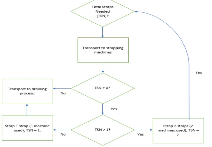
The processing time of the strapping machine depends on the number of straps needed to strap one bundle of tubes, which depends on the length and weight of the tubes in the bundle. Figure 14 visualizes the relation between the number of straps and processing time: the more straps needed, the more steps the bundle of tubes needs to go through, which implies a longer processing time. In the case of the 273 and 323 with a length of 12 meter, 6 straps are used, so the bundle needs to pass the two strapping machines 3 times. The bundle goes through the following steps:
(1) Transport 1 (T1): transport to the strapping machines. The bundle is placed in the machines and is ready to be strapped.
(2) Strapping 1: The bundle is strapped for the first time.
(3) Transport 2 (T2): The bundle moves in the strapping machines and is positioned for the strapping of the second pair of straps. During transport 2, the strapping machines are refilled with new strapping material.
(4) Strapping 2: The bundle is strapped for the second time.
(5) Transport 3 (T3): The bundle moves through the strapping machines and is positioned for the strapping of the third pair of straps. During transport 2, the strapping machines are refilled.
(6) Strapping 3: The bundle is strapped for the third time.
[image:26.595.118.473.164.410.2](7) Transport 4 (T4): The bundle is finished and is transported to the draining queue The total process takes 70 seconds, which implies a processing speed of 21 meters of tubes per minute. Therefore, the processing speed of the whole bundling process equals 21 meters of tube per minute.
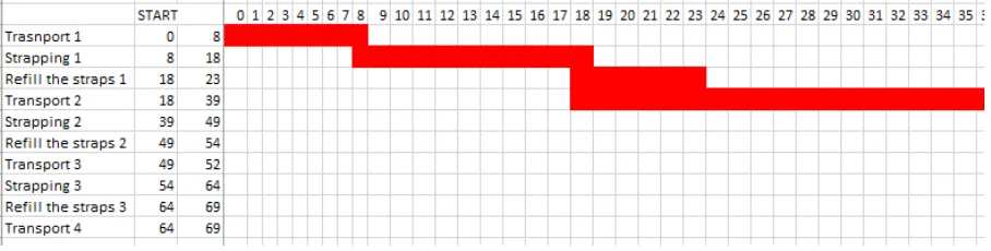
20 Time samples of each step in the strapping process have been gathered to gain a deeper
[image:27.595.72.526.150.265.2]understanding of the process performance. Figures 15 and 16 present the processing time of each of the steps involved. Figure 15 shows the first 35 seconds and figure 16 shows the second 35 seconds. As shown in the figures, some processes take place simultaneously (transport and refilling the strapping machines).
[image:27.595.76.529.292.402.2]Figure 15: Timeline strapping process; interval 0-35 seconds
Figure 16: Timeline strapping process; interval 35-70 seconds
Looking at figure 15, it becomes evident that transport 2 takes a relatively long time. It takes 21 seconds, which is 27 % of the total processing time. In those 21 seconds the bundle of tubes is transported over 3.5 meters. Covering those 3.5 meters, take 21 seconds, because the strapping process is hindered by the process downstream of the strapping machines: placing of the previously strapped bundle in the draining queue. Normally it would take approximately 5 seconds to cover 3.5 meters, due to the hinder it takes 21 seconds. Another important thing to note is that one cycle of strapping (placing + refill) takes 15 seconds in total, which is 21% of the total strapping time. The bundle of tubes needs to go through 3 cycles, which adds up to 45 seconds of strapping.
So far, the focus has been on the processing time. This paragraph will focus on the other variable that affects the speed: meters of tube processed. When bundling 2 tubes in one bundle, only 24 meters of tube are processed. 24 meters of tube in one bundle is a very short length compared to other production scenarios. The processing time does not depend on the number of tubes per bundle, so ideally, we would bundle as many tubes as possible. The ‘solution generation’ chapter
goes into whether this is possible or not.
4.4
Current Reality Tree
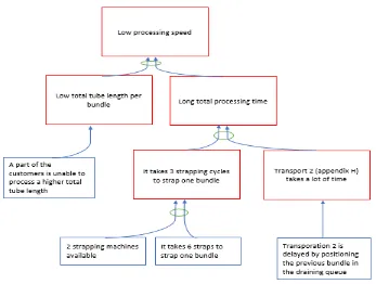
21 The UDEs are presented in the red rectangles. The cause-effect relationships between the UDEs have
been added, as well as some ‘neutral causes’. The neutral causes (in blue) are the arguments that Tata Steel Tubes has given me for their design of the strapping process. These arguments will be re-evaluated in the solution generation chapter, since they might be invalid.
The current reality tree presents 3 potential problems: 1. low total tube length per bundle
2. strapping cycles per bundle 3. transport 2 takes a lot of time.
It also shows the relationship between processing time, total tube length per bundles and processing speed, which will be used in the solution generation chapter.
4.5
Intermediate conclusion: RQ1
RQ1: What is the cause of the underperformance on the speed at which the tubes arrive in the outside storage of the M-93 at Tata Steel Tubes?
The output speed of the M-93 is set by the bottleneck of the M-93. The workstations in the research population have been analysed on their performance on the processing speed, which determines the throughput of each workstation. The bundling workstation has a processing speed of 21 meter per minute and therefore it has been identified as the constraining workstation. The bundling process consists of two processes: creation of the bundle shape (MAIR) and strapping the bundle. The bottleneck turned out to be the strapping process. Time samples of the strapping process were taken and a timeline was set up. The timeline provided insights in the critical steps in the strapping process. Additionally, a current reality tree was used to outline the cause-effect relations between the undesired effects and (root)causes. The analysis led to multiple causes of the problem. However, the most prominent factor is that the strapping process is hindered by the subsequent step in the production line (placing the bundle in the draining queue). The distance between the strapping process and the draining queue is very small and when the bundle is strapped, it moves through the strapping machines which results in the bundle to protrude to either the MAIR-side or the
[image:28.595.138.485.87.349.2]22 side of the machine. Since the distance, between the strapping machine and the draining queue is rather small, the bundle cannot protrude to the draining-side too much, when the previously strapped bundle is being processed. This is orchestrated by sensors. At the moment, the process of placing the bundle in the draining queue takes up too much time, therefore the sensor that
23
5
Solution generation
The aim is to increase the processing speed of the strapping process such that it meets the processing speed of the tube mill (appendix A). The CRT sets the direction to achieve this aim:
1. Decrease the time interval in which a certain amount of tubes is processed 2. Increase the amount of tubes that is processed during a constant time interval. The CRT shows the following potential conflicts:
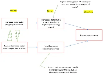
1. Increase total tube length, to increase speed versus not increase total tube length, because some customers cannot process bundles with a higher total tube length.
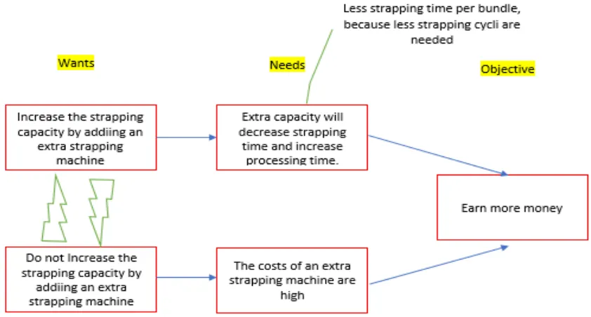
2. Add an extra strapping machine, to increase processing speed versus not add an extra strapping machine, because of extra costs.
3. Use less straps to strap one bundle to decrease processing time versus strap with the current number of straps, because of the strap strength.
The CRT also points to another improvement possibility to decrease the processing time: decrease T2. The interventions can be implemented as a combination or individually.
5.1
Evaporation clouds
Setting up de EC start with the conflicting wants that result from two needs that both should serve the overall objective. In the previous chapters, the goal is described as an increase in processing time of the bottleneck such that it will meet the processing speed of the tube mill. The motive behind this goal is to produce more tubes and by doing so, earn more money. The objective used in the ECs is
‘earn more money’. This decision has been made, because the analysis of the conflicting arguments will be more accurate. If the arguments were analysed based on the objective to increase the processing speed, some profit affecting factors would be excluded from the analysis and the achievement of the overall aim would be in jeopardy.
5.2
Bottleneck: downstream process hinders strapping
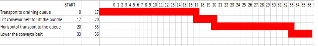
The most prominent constraining factor is the delay of Trasnport 2 (T2; figure 15). T2 is delayed, because the previously strapped bundle must be placed in the queue of the draining process. Starting from the point in time where the new bundle can enter the strapping machine, it takes approximately 39 seconds until the second pair of straps can be strapped (figure 18). The steps that must be taken to place the previously strapped bundle in the draining queue are:
1. Further transport, such that the strapped bundle is accurately placed in front of the draining queue
2. Lifting the strapped bundle by lifting the whole conveyor belt, such that the horizontal transport toward the draining queue is possible
3. Horizontal transport to the draining queue. 4.
[image:30.595.59.587.647.725.2]5. Lowering the conveyor belt to receive the next strapped bundle.
24 A timeline based on samples can be found in figure 18. The total time it takes to place the previously strapped bundle in the draining queue is approximately 36 seconds. It is important to note that T2 is only hindered by placing the previous bundle in the draining queue if the subsequent bundles follow each other closely, which only is the case when the strapping process is the bottleneck.
The transport from the strapping machine to the draining queue (in figure 18: ‘transport to draining queue’) takes up 47% of the total processing time. The average transport time to the draining queue is 17 seconds. One of the reasons that it takes so much time is that the inline transportation of the strapping machine is connected to the transportation to the draining queue. Both the transportation processes are driven by the same computer. The result of this connection is that when the
transportation in the strapping process stops, the transport to the draining queue stops as well. This is problematic, because the moment that the bundle is strapped, which implies that the bundle in the strapping machines is stopped, the transport to the draining queue is stopped. This is
unnecessary. If two independently driven transport sections are created, one inline transport section for the strapping process and one transport section to the draining queue, stopping the strapping process will not result in stopping the transport to the draining queue. The transport could be orchestrated by a variable frequency drive, which regulates the operating speed more fluently than the current reality (two options: on or off). A small engine is used to lift the conveyor belt. The processing time of lifting and lowering the conveyor belt can be decreased by changing the gear ratio. This might imply that a stronger engine is needed. Figure 18 shows that the lifting and lowering of the conveyor belt only takes up 6 seconds (in total), which is approximately 17% of the total cycle time. An engine in combination with a pulse counter is used to transport the bundle horizontally toward the draining queue. The engine has enough capacity to increase the
transportation speed, however the pulse counter will not be accurate enough and since it measures the distance over which the bundle is transported it must be accurate. Transporting the bundle horizontally takes up 36% of the total processing time. All the information above is gathered in an interview with Jacco Jansen and through time sampling. Splitting up the transportation in two sections (strapping and draining) and a more accurate pulse counter will have the biggest impact, because the steps affected by those interventions take up the biggest part of the total processing time. I assume that the processing time of placing a bundle in the draining queue can be decreased with 25%, if the transport speed to the draining queue and the horizontal transport speed are increased. In the current situation, the bundle in the strapping machine is approximately hindered for 16 seconds by the placing of the previous bundle in the draining queue. A decrease in processing time of 25% implies that the time the bundle is hindered decreases to approximately 6 seconds. Ideally, the bundle is not hindered at all. To achieve the situation the processing time of placing a bundle in the draining queue should be decreased by 40%. Further research should be conducted to determine whether a decrease of 40% is achievable.
The intervention proposed above, could easily be combined with one of the proposed improvements below. These combinations will be evaluated in the experiments of the simulation study (described further in the report).
5.3
Additional improvement possibility 1
25 Figure 19: Evaporation cloud on additional tube length
The Evaporation Cloud in figure 19 was set up to evaluate the arguments that Tata Steel Tubes presented me and to create an overview of the restrictions involved in the decision to come up with the most effective solution considering the restrictions.
There are two restrictions to this intervention:
1. The solution is applicable for the 323 and 273 for a wall thicknesses up to 5 mm. Otherwise the bundles become too heavy, which will result in dangerous situations (during transport & loading/unloading the bundles). This restriction is based on the judgment of Chris van Meeteren.
2. Only a part of Tata Steel Tubes’ customer can process bundles consisting of 5 tubes. This
restriction is elaborated upon below:
After a second meeting with Chris van Meeteren, it became evident that some customers are unable to process 5 tubes in one bundle. If Tata Steel Tubes would decide to only offer bundles of 5 tubes, some customers and the corresponding profit will be lost. On the other hand, the processing time of the bottleneck would be increased and thus the output rate of the whole chain would increase, which implies an increase in produced tubes per time period. The increased production quantity implies a higher profit. It might seem like you will inevitably loose a part of the potential profit, regardless the decision that is made. However, I propose to identify the customers that cannot process bundles of 5 tubes and inform them on the situation. Two further courses of action are possible:
1. Offer bundles of two tubes only to the customers that are unable to process bundles of 5 tubes. The other customers, will receive the tubes in bundles of 5 tubes.