Customer purchase prediction through machine learning

Faculty of Electrical Engineering,

Mathematics & Computer Science

Customer purchase prediction

through machine learning

Hannah Sophia Seippel M.Sc. Thesis

March 2018

Graduation committee:

be mentioned due to confidentiality reasons, but who will surely know that he is addressed. Thank you for providing me with the topic for this master thesis that con-nects Data Science with Business, making it a perfect fit for my degree in Business Information Technology with a focus on Business Analytics. And a further thanks for supporting me along the way with guidance and good advice.

A thank you goes to the University of Twente, for offering this interesting Master program and making an internship and a master thesis abroad possible. Of course, I would also like to thank my two supervisors Dr. Chintan Amrit and Arun Ramakr-ishnan for providing helpful feedback and support and also Dr. Mannes Poel who agreed on being my second university supervisor on such short notice.

Finally and most importantly, I would like to thank my family and friends, who have always shown great support, especially my parents without whom none of this would have been possible and Fabian who always believes in me.

Due to today’s transition from visiting physical stores to online shopping, predicting customer behavior in the context of e-commerce is gaining importance. It can in-crease customer satisfaction and sales, resulting in higher conversion rates and a competitive advantage, by facilitating a more personalized shopping process. By uti-lizing clickstream and supplementary customer data, models for predicting customer behavior can be built. This study analyzes machine learning models to predict a pur-chase, which is a relevant use case as applied by a large German clothing retailer. Next, to comparing models this study further gives insight into the performance dif-ferences of the models on sequential clickstream and the static customer data, by conducting a descriptive data analysis and separately training the models on the dif-ferent datasets. The results indicate that a Random Forest algorithm is best suited for the prediction task, showing the best performance results, reasonable latency, of-fering comprehensibility and a high robustness. Regarding the different data types, models trained on sequential session data outperformed models trained on the static customer data by far. The best results were obtained when combining both datasets.

special offers. By utilizing clickstream and additional customer data, predictions can be carried out, ranging from customer classification, purchase prediction, and recommender systems to the detection of customer churn. A variety of machine learning models and data are available to conduct these kinds of predictions.

Research Problem

Categorizing whether a web shop session will end in a purchase or not, is a rel-evant use case in the context of predictions in e-commerce. This categorization followed by the display of gift cards to non purchasing customers, to convince them of a purchase nonetheless, has proven to increase turnover of a large German cloth-ing retailer. A variety of possible prediction models as well as different data sources exist to carry out such predictions. This paper aims at retrieving well-suited pre-diction models and comparing their performances across different data types, such as static and dynamic data, to establish how customers can be best classified as buying or no buying. This results in the following research question:

How can a customer in a web shop be categorized as a buying or no buying cus-tomer?

Methodology

This research was structured based on the Cross Industry Standard Process for Data Mining (CRISP-DM) methodology. Suitable models, being boosted tree,

dom Forest (RF), Support Vector Machine (SVM), Feed-forward Neural Network (FNN), Logistic Regression (LR) and Recurrent Neural Networks (RNN), were identi-fied through a literature research. Following, algorithms were trained on three differ-ent datasets, the sequdiffer-ential session data, the static customer data and a combined dataset, then evaluated and compared based on different performance metrics, pre-diction latency and comprehensibility. The RNN was further trained on datasets with varying degrees of required feature engineering. All algorithms as well as the eval-uation and comparison were implemented in Python.

Results

The obtained results indicate that the RF performed best while showing reason-able prediction latency. Regarding the comprehensibility, no difference between the different algorithms was observed. The performance of different datasets shows that a combined dataset leads to the best results, where customer information en-hances the results only slightly. An overview of the results regarding the different datasets and algorithms concerning the ROC AUC value can be observed in Table 1. Further, a promising effect regarding time-consuming feature engineering was observed for the RNN, where fewer and less engineered features led to better re-sults than a larger amount of more heavily engineered features as used for the other algorithms.

Table 1: ROC AUC results for all algorithms and datasets.

Algorithm/ Data Type Combined Data Sequence Data Customer Data

Boosted tree 0.79 0.78 0.64

RF 0.82 0.81 0.67

FNN 0.73 0.67 0.67

SVM 0.67 0.74 0.39

LR 0.8 0.78 0.65

RNN 0.74 0.74 0.66

Conclusion

2.1 SVM: Maximum margin hyperplane . . . 11

2.2 Architecture of FNN . . . 13

2.3 Architectures of an FNN versus an RNN . . . 15

2.4 RNN versus vector-based methods . . . 16

3.1 CRISP-DM steps . . . 21

3.2 Confusion Matrix . . . 23

3.3 Exemplatory Receiver Operating Characteristic (ROC) . . . 25

4.1 Landmark example . . . 28

4.2 Analysis of weekday variable . . . 30

4.3 Analysis of entry channel variable . . . 31

4.4 Analysis of device variable . . . 32

4.5 Analysis of customer identification variable . . . 33

4.6 Analysis of last device variable . . . 34

4.7 Analysis of gender variable . . . 34

4.8 Analysis of age variable . . . 35

4.9 Feature importance . . . 40

5.1 Grid search for RF . . . 43

5.2 Grid search for SVM . . . 45

6.1 ROC AUC results . . . 50

6.2 Latency results for 100 data points . . . 56

6.3 Prediction throughput for each algorithm . . . 56

6.4 Buying behavior predicted by RF . . . 58

6.5 Buying behavior predicted by RNN . . . 58

A.1 Hyper-parameters of boosted tree . . . 76

A.2 Hyper-parameters of RF . . . 76

A.3 Hyper-parameters of RF . . . 77

A.4 Hyper-parameters of LR . . . 77

A.5 Architecture of FNN . . . 77

1 ROC AUC results . . . v

2.1 Summary of literature . . . 7

3.1 CRISP-DM phases . . . 21

4.1 Features used for DT, SVM, FNN and LR . . . 37

4.2 Features used for RNN . . . 38

6.1 Results of complete dataset . . . 49

6.2 Results of sequence dataset . . . 51

6.3 Results of customer dataset . . . 52

6.4 RNN results on RNN dataset . . . 54

6.5 ROC AUC of the prediction results split by day . . . 54

6.6 Percent of correct answers split by device . . . 55

6.7 Percent of correct answers split by gender . . . 55

B.1 Confusion Matrices of results . . . 79

C.1 Results of the Deep Forest implementation on the complete dataset. . 81

FNN Feed-forward Neural Networks HMC Higher-order Markov Chains KNN K-nearest Neighbor

LR Logistic Regression LSTM Long short-term memory

RF Random Forest

ROC Receiver Operating Characteristic RNN Recurrent Neural Networks

SVM Support Vector Machines PCA Principal Component Analysis

Preface ii

Abstract iii

Management summary iv

List of Figures vii

List of Tables ix

List of acronyms x

1 Introduction 1

1.1 Motivation . . . 1

1.2 Problem definition . . . 3

1.3 Report organization . . . 5

2 Literature review 6 2.1 Binary Classification . . . 6

2.2 Learning algorithms for binary classification . . . 8

2.2.1 Decision Trees . . . 8

2.2.2 Support Vector Machines . . . 10

2.2.3 Logistic Regression . . . 12

2.2.4 Feed-forward Neural Networks . . . 12

2.2.5 K-nearest Neighbor . . . 13

2.2.6 Recurrent Neural Networks . . . 14

2.2.7 Higher-order Markov Chains . . . 16

2.3 Implications . . . 17

2.3.1 Algorithm performance . . . 17

2.3.2 Dataset performance . . . 18

2.3.3 Literature gap . . . 19

4.2 Data pre-processing . . . 28

4.3 Data understanding . . . 30

4.3.1 Sequence dataset . . . 30

4.3.2 Customer dataset . . . 33

4.4 Features . . . 35

4.4.1 Feature engineering . . . 36

4.4.2 Feature selection . . . 39

5 Implementation 41 5.1 Implementation and hyper-parameter tuning . . . 41

6 Results 48 6.1 Performance results . . . 48

6.1.1 Results on RNN data . . . 53

6.1.2 Robustness of results . . . 53

6.2 Latency results . . . 55

6.3 Comprehensibility . . . 57

7 Discussion 59 7.1 Principal findings . . . 59

7.2 Limitations . . . 64

7.3 Future work . . . 65

8 Conclusion 67 References 70 References . . . 70

Appendices A Algorithm Implementation 76 A.1 Boosted tree hyper-parameters . . . 76

A.2 Random Forest hyper-parameters . . . 76

A.3 Support Vector Machine hyper-parameters . . . 77

A.5 Feedforward Neural Network Architecture . . . 77 A.6 Recurrent Neural Network Architecture . . . 78

B Results 79

B.1 Confusion Matrices . . . 79

chapter. Research in this area is motivated in the first part (Section 1.1). Resulting, a research question, and sub-questions are formulated in Section 1.2. Finally, the structure of the thesis is outlined in Section 1.3.

1.1 Motivation

As a result of today’s knowledgbased economy and the information society, e-commerce is becoming increasingly popular all over the globe. The most common type being the Business-to-Customer trade, typically represented as online stores, displacing physical stores quickly (Suchacka & Chodak, 2016). The transition from physical to online shopping can be inferred by numbers such as an increase in to-tal retail sales in Germany of 3% in 2016, whereas the e-commerce sales rose by an estimated 12.5% to 58.52 billion dollars and are expected to exceed 86 billion dollars at the end of 2021 (Retail Ecommerce in Germany: A Major Digital Market Growing in Size and Sophistication, 2017). The rapid growth of e-commerce has

transformed the shopping process as a whole and along with it the traditional buyer-merchant relationships. This change is accompanied by challenges that companies need to address. Such challenges entail more competition and a volatile relation-ship between customers and merchants since customers and their preferences are no longer personally known, resulting in less loyal customers. Therefore, attract-ing customers, gainattract-ing their trust and retainattract-ing them becomes a main objective in modern e-commerce (Nakayama, 2009; Salehi, Abdollahbeigi, Langroudi, & Salehi, 2012). Web shop visitors leave more traces than ever before. Large amounts of per-sonal information as well as clickstream data, recorded during each web shop visit, are collected, connected and stored for analysis with data mining techniques.

edge retrieved from these analyses can improve customer satisfaction, by making the shopping process more efficient, more engaging and increasingly personalized (Magrabi, 2016), mitigating the risks associated with the aforementioned challenges. In the long run, this can lead to a competitive advantage resulting from a higher con-version rate and increased turnover (Hop, 2013; Suchacka & Chodak, 2016).

The analysis of customer purchase behavior dates back to the beginning of e-commerce (Bellman, Lohse, & Johnson, 1999) and has many applications nowa-days. Examples are item recommendations for customers (Y. Tan, Xu, & Liu, 2016; Hidasi, Quadrana, Karatzoglou, & Tikk, 2016), the classification of customers into certain categories such as buyers, visitors, etc. (Moe, 2003; Fajta, 2014), predicting the purchase probability in order to offer a higher quality of service to customers that are more likely to buy (Lo, Frankowsik, & Leskovec, 2014; Korpusik, Sakaki, Chen, & Chen, 2016; Suchacka & Templewski, 2017; Lang & Rettenmeier, 2017) and the timely detection of customer churn in order to prevent such (Xie, Li, Ngai, & Ying, 2008; Castanedo, Valverde, Zaratiegui, & Vazquez, 2014). This thesis is similar to the detection of customer churn, being concerned with predicting the abortion of a shopping process in order to prevent it. Prevention is possible through, for example, showing recommended items or displaying gift cards to motivate a purchase. Pre-dictions of customer actions are often based on personal customer data, clickstream data and supplementary data from other sources. Various machine learning meth-ods exist to perform classification on the collected clickstream data. Examples are regular machine learning models such as Logistic Regression (LR), Support Vec-tor Machines (SVM), Decision Trees (DT), Random Forest (RF) and Feed-forward Neural Networks (FNN) as well as stateful models such as Higher-order Markov Chains (HMC) and Recurrent Neural Networks (RNN).

Motivated by the increasing importance of classifying customer behavior and a large number of possible prediction models and data sources, this thesis aims at implementing and comparing suitable models trained on different datasets to iden-tify the most appropriate one for predicting the abortion probability of a web shop visitor. Hence, a binary classification task of a visitor belonging to the aborting or not aborting category. This classification followed by the display of gift cards in order to persuade the visitor to stay in the web shop has been tested by a large German clothing retailer in an A/B test and showed an increased conversion rate from 8% to 10% under assumptions of a cost-benefit analysis. It is, therefore, a suitable and relevant use case for testing classification models and different data types in the context of e-commerce.

analysis is expected to give reasoning about the bad performance of static customer data compared to dynamic clickstream data.

In the study of Lang and Rettenmeier (2017), an RNN was implemented to pre-dict the probability of a purchase occurring within a web shop session. The study claims that RNNs, being stateful models equipped with a memory, provide a possibil-ity of reducing labor-intensive feature engineering in the context of sequential data. Lang and Rettenmeier do not include a comparison about how RNNs perform on datasets with different degrees of feature engineering, and do, therefore, not prove if less feature engineering does indeed show as good results as heavily engineered features. Resulting from this and since the sequential clickstream data seems to be a natural fit for RNNs, this study aims at training an RNN on datasets with dif-ferent levels of feature engineering, to establish how well RNNs perform on less engineered features. This shows how RNNs might offer the possibility to reduce feature engineering, which is very important for e-commerce since it is typically a time-consuming task that requires a lot of expert knowledge.

Finally, after obtaining the results, these are tested for their robustness, to display how different conditions, such as the used device or day of the week, could influence the models’ performance. This improves on the findings in literature since none of the reviewed papers analyze how the obtained results might behave under different conditions, even though this is important to assess since it helps to understand how a model would perform under real conditions after deployment.

1.2 Problem definition

Resulting from the facts stated in Section 1.1, in this thesis, machine learning models are identified and implemented for solving the task of classifying a web shop visitor as aborting or non aborting, in the following referred to as no buying and buying sessions.

performance, latency, and comprehensibility. Latency is important since in the use case, predictions have to be conducted in real-time and model comprehensibility is considered since the demand for explaining decisions made by machine learning models is rising. The boosted tree model that is already being used by the German clothing retailer, will act as a baseline for the comparison of the different algorithms. To provide further insight and reasoning about the varying performances on different datasets, an exploratory data analysis on the clickstream and static customer data is conducted.

An RNN, representing the class of stateful machine learning models, is addition-ally trained on datasets, which required fewer feature engineering, to show if stateful models provide good results while reducing the need for feature engineering.

After obtaining the results of the different models on all datasets, the models are tested for their robustness to different conditions. Examples of such conditions are the gender of the visitor or the device on which the web shop was visited. This anal-ysis indicates how the models will perform under real conditions after deployment.

Deployment is out of scope for this research and can only be regarded as an implication if a tested model outperforms the baseline model.

From all of the previously mentioned points the research question as stated be-low results:

Research Question: How can a visitor in a web shop be categorized as a buying or no buying?

Five subquestions are needed to completely answer the main research question and are stated in the following:

Sub Question 1:How can an exploratory data analysis provide insight into the prediction problem?

Sub Question 2: Which machine learning model is best suited to solve the prediction problem?

Sub Question 3: How do different data types, such as dynamic clickstream and static customer data, influence the models’ performance?

1.3 Report organization

Literature review

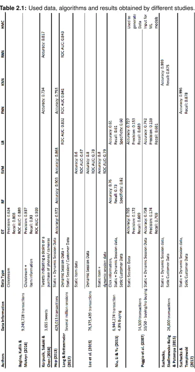
This chapter reviews the results and algorithms used by studies concerned with a similar binary classification problem as the one at hand. To create a broader under-standing of the problem and the different algorithms, binary classification and the algorithms used for solving it are each explained before reviewing their application and performance in literature. All reviewed literature is summarized in Table 2.1, showing details on the data and results obtained in each study. Looking at the table one has to keep in mind that comparing results across studies is difficult since dif-ferent data types, evaluation metrics, evaluation thresholds, etc. were used. Finally, a gap analysis of the reviewed literature is conducted.

2.1 Binary Classification

Data mining has various applications with classification being the most common one. Being a predictive analytics task, the aim of classification is to predict a categorical target variable from a set of input variables. This target variable can be expressed either through various categories or be of binary nature (Kotu & Deshpande, 2014). The task at hand is a binary classification task since the target variable has two cat-egories: buying andno buying. In order to predict the target variable a generalized

relationship between input and target variable is learned from a labeled dataset. It is then applied to new data for classification. Learning algorithms should both fit the training data and generalize well over new data (P. Tan, Steinbach, & Kumar, 2005). Various machine learning algorithms exist that have different methods of extracting this relationship.

2.2 Learning algorithms for binary classification

The most common type of machine learning algorithms for a binary classification task are vector-based methods. Belonging to this category are DTs, RFs, SVMs, LR, and FNNs. The baseline model of this study also associates with this category being part of the DT algorithms. Common to these algorithms is to learn supervised with a set of feature vectors and corresponding outputs (Heaton, 2016). They are eager learning models, where a classification model is constructed based on a given training dataset before new data is classified according to the model. The opposites are lazy learners, such as the K-nearest Neighbor (KNN) algorithm, where training data is simply stored and a test data point is awaited for classification (Han, Pei, & Kamber, 2011).

All of the above-mentioned methods are stateless machine learning algorithms; they do not have any memory and always return the same answer given the same input. This is well-suited for most classification tasks, however, it is difficult to model patterns over time, since the different states have to be modeled through complex feature engineering, creating inaccuracies and increasing complexity by raising the number of input features. Nevertheless, the ability to model time sequences and extract patterns over time can be useful for the research at hand, since the click-stream data used in this study is of sequential and time-dependent nature. Fortu-nately, stateful models exist, equipped with a memory, to remember previous states and to extract sequential patterns without the need for engineering time-dependent features explicitly. Examples of such models are RNNs and HMCs. All of the men-tioned algorithms are explained below, each followed by their applications and per-formances in literature.

2.2.1 Decision Trees

Boosted DTs belong to the ensemble methods, consisting of more than one DT. Here, a sequence of trees is built, where each tree results from the prediction resid-uals of the previous tree (Friedman, 2002). An example for such a method is the baseline model used for this study. Boosted DTs have proven to be a very powerful method for predictive analytics by winning a lot of Kaggle machine learning compe-titions (Kaggle – The Home of data Science and Machine Learning, 2017), but are

less comprehensible than simple DTs, since they consist of many trees.

Random Forest

Bagging is another example for ensemble trees, where many large trees are fit to the bootstrap re-sampled versions of the data and are classified by majority vote (Breiman, 1996). RF improves on Bagging by de-correlating the trees. After each tree split a random sample of features is chosen and only these are considered for the next split. The results are again based on the majority vote of the single trees. By using a large number of classifiers, Bagging and RFs, improve on the weaknesses of non-ensemble DTs, such as robustness and over-fitting. They train faster than the boosted trees but need more time for the prediction (Breiman, 2001). Neverthe-less, Bagging and RFs still depend on feature engineering and cannot model time dependencies.

DTs show great results throughout literature being applied to very similar prob-lems as this research. Bogina et al. (2016), for example, used different DT algo-rithms to classify a session as a buying or no buying session. Next to clickstream data also a setup with additional data about item sales statistics was used, which increased the prediction performance. In the case where only clickstream data was used, being the closest to our use case, a Bagging RepTree showed the best re-sults. It was implemented in Weka, a tool that supports data analysis with different machine learning techniques (Frank, Hall, & Witten, 2016) and showed a preci-sion of 0.824, a recall of 0.808, an F1-score of 0.806 and a ROC Area under the curve (AUC) of 0.889.

transac-tions were used for training this model. The authors tested separately for static ses-sion information and static and dynamic sesses-sion information combined. The results show that combining static and dynamic session data only increased the prediction performance slightly. The results further show that the J48 model, a DT, outper-formed an LR classifier with a recall of 0.708 compared to a recall of 0.681.

In the prudsys Datamining Cup 2013, the challenge was to classify buying ver-sus no buying sessions from clickstream data (DMC 2013, 2013), where the training

dataset contained 429,013 data points. The winning team from the University of Dortmund achieved an accuracy of 0.972 by using Bagging of 600 C4.5 DTs (Hop, 2013). Hop also competed in the prudsys Datamining Cup 2013 and compared RFs with SVMs and an FNN. RFs outperformed the other two methods with an accuracy of 0.903, the SVM showed the second best accuracy with 0.868, whereas the FNN only achieved an accuracy of 0.755. Next to the high accuracy Hop also mentions other advantages of the RF method: Compared to SVMs the computational effort of training is low and it requires minimal hyper-parameter tuning making it easy and fast to use.

Lastly, Niu, Li, and Yu (2017) also estimated purchase probabilities with RFs while not mainly focusing on clickstream data itself, but on search queries and click positions. For building the model they included information about mouse clicks, static and dynamic session data as well as static customer data. To train and evaluate the model a rather large amount of 1,530,738 records was used. Their study shows that a RF outperformed the LR with an accuracy of 0.76, a sensitivity of 0.73 and a specificity of 0.82, compared to results of 0.61, 0.61 and 0.60 respectively. Next to the prediction results, they also show some descriptive statistics of the customer shopping behavior such as the average amount of formulated queries being 8.3 and that a visitor spends around three minutes on an article detail page.

2.2.2 Support Vector Machines

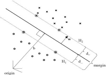
An SVM separates two classes by fitting a hyperplane between them. Doing this, only one hyperplane is used, which differs from DTs where a hyperplane is added after each split. In cases where multiple separating hyperplanes can be found, the SVM detects the maximum-margin hyperplane, maximizing the distance to data points of both classes. Such a hyperplane is shown in Figure 2.1. This leads to a higher generalizability and therefore to better test accuracies.

con-Figure 2.1: Optimal separating hyperplane with maximal margin. Retrieved from Hofmann (2006).

duct non-linear classification (Cortes & Vapnik, 1995). Four basic kernel functions are listed below (Hsu, Chang, & Lin, 2003):

Linear=K(xi, xj) =xTi xj (2.1)

P olynomial=K(xi, xj) = (γxixj +r)d, γ >0 (2.2)

Radial basis f unction(RBF) = K(xi, xj) = exp(−γ||xi−xj||2), γ >0 (2.3)

Sigmoid=K(xi, xj) = tanh(γxixj+r) (2.4)

WhereK(xi, xj)is the kernel function, mapping the training vectors xi into a higher

dimensional feature space. y, r and d are kernel specific parameters (Hsu et al., 2003).

Regarding their performance, SVMs show a high accuracy as well as fast pre-diction times. They further work very well with high-dimensional data input. Disad-vantages are long training times and their difficulty to be interpreted. Further, next to feature engineering, also hyper-parameter tuning is required, which can be difficult and time-consuming (Han et al., 2011).

the complete dataset and only the session data are very similar, indicating that the static item information does not contain high predictive power. The results on the complete data show an accuracy of 0.8, a ROC of 0.79, a precision of 0.74, a recall of 0.92 and an F1-score of 0.82.

2.2.3 Logistic Regression

LR, also called Logit regression, belongs to the class of generalized linear models and is used to predict categorical target variables. This is achieved through a logistic function, which has the shape of a sigmoid curve, taking values between 0 and 1. This function is modeled by combining input values linearly with coefficients, as shown in Equation 2.5. Whereyis the output, b0 the bias term andb1 the coefficient

for the input valuex(Russell & Norvig, 1995).

y= e

b0+b1x

1 +eb0+b1x (2.5)

Every column of the input vector learns a coefficient from the training data through maximum-likelihood estimation (Hastie, Tibshirani, & Friedman, 2002). LR is very fast regarding prediction and training times, it is, hence, one of the most popular ma-chine learning algorithms for binary classification. It, nevertheless, requires feature engineering and the encoding of categorical variables. It is also sensitive to noise, therefore, outliers should be removed before the training. Further, LR does not per-form well on highly correlated input factors. Hence, it can be helpful to only use prin-cipal components, linearly uncorrelated variables, for the regression (Jolliffe, 1982). This can be achieved through a Principal Component Analysis (PCA), a method to extract the principal components from a set of possibly correlated variables.

LR has been used in a variety of the reviewed papers but has always been outperformed by other machine learning methods, shown in the above-mentioned studies of Poggi et al. (2007) and Niu et al. (2017). Similar findings were obtained by a study from Lang and Rettenmeier (2017), where an RNN outperformed the LR in predicting the purchase probability based on clickstream data, static session data, and customer data with a ROC AUC of 0.843 and 0.832 respectively.

2.2.4 Feed-forward Neural Networks

Figure 2.2: An FNN with two hidden layers, three input and two output nodes. Re-trieved from A Practical Introduction to Deep Learning with Caffe and Python(2016).

node in a layer connects to all nodes of the previous layer. An exemplary architec-ture can be seen in Figure 2.2. The connections have different weights assigned, which are generated during the learning phase, for example via back-propagation. Every node has an activation function and only fires according to this function. Out-put is the probability of each class, which add up to one. With enough hidden units, an FNN can approximate any function. From a statistical point of view, FNNs per-form a nonlinear regression. Such neural networks have the disadvantage of long training times and little comprehensibility. Next to feature engineering, they require hyper-parameter tuning. Nevertheless, they have shown very good performances throughout literature and generalize well to unseen patterns, while being tolerant to noisy data (Han et al., 2011).

Other than the before mentioned research by Hop (2013), which displayed a bad performance for FNNs, Suchacka and Templewski (2017) were able to achieve a high accuracy (0.996) and recall (0.878) for an FNN on clickstream data to predict purchases in sessions. They used static and dynamic session data as well as static customer data to train the model. The large performance difference to the paper of Hop might be due to the fact that Hop used a rather simple FNN with only one hidden layer and that different data was used to train and test the models in the two papers.

2.2.5 K-nearest Neighbor

All of the stored training instances correspond to points in ann-dimensional feature

space. A point’s nearest neighbors are defined by distance measurements, most commonly Euclidean distance. An unlabeled test data point will be assigned the la-bel most common amongst itsk-nearest neighbors. The advantages of this method

are its robustness to noisy data and a very fast training speed. Disadvantages are an increased complexity of dimensionality through irrelevant features and therefore a decreased performance, highlighting the importance of feature engineering, longer prediction times compared to eager learning models and a low comprehensibility with high-dimensional input.

The KNN model has been applied regularly in e-commerce regarding recom-mender systems, where products are recommended to a web shop visitor based on the preferences of its nearest neighbors. For classifying customer behavior on the other hand only one study by Suchacka, Skolimowska-Kulig, and Potempa (2015) could be found. The aim of the research was to classify customer web shop ses-sions in buying or browsing sesses-sions. As a model, a KNN algorithm was used with clickstream data split by sessions as input. 26,000 records were used for training and 13,000 for testing. Different configurations were tested, with an 11-NN model showing the best results, with a sensitivity and accuracy of 0.875 and 0.9985 re-spectively.

2.2.6 Recurrent Neural Networks

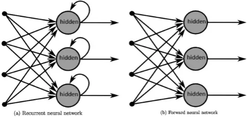
Figure 2.3: On the left an architecture of an RNN showing backward connections compared to an FNN with only forward connections on the right. Re-trieved from Mulder et al. (2015).

Frasconi, 1994; Korpusik et al., 2016). A solution to the vanishing gradient prob-lem offers the Long short-term memory (LSTM) network. In LSTMs neurons are replaced by memory cells. These cells operate through gates that manage the cells’ input, output and state. These gates are activated with a sigmoid function making the information flow through the cell conditional (Brownlee, 2016). As a result, in-formation that increases prediction accuracy is kept in the memory cell, solving the vanishing gradient problem (Hochreiter & Schmidhuber, 1997).

As mentioned above, RNNs and LSTMs decrease the amount of feature engi-neering and can model time dependencies of the input data. The paper of Lang and Rettenmeier (2017) shows how the influence of different customer actions on the prediction outcome can be visualized, providing a high interpretability. Drawbacks are both extended prediction and training times compared to other machine learning methods. They further require hyper-parameter tuning, which can make architec-tural choices complex (Lang & Rettenmeier, 2017).

RNNs are applied in the most recent studies on predicting customer behav-ior. Lang and Rettenmeier (2017) used clickstream data and customer information to predict the purchase probability of a customer with LSTMs. The model outper-formed the also tested FNN and LR with a ROC AUC of 0.841, 0.832 and 0.843 for FNN, LR and RNN respectively. On the downside, RNNs need a lot of data and time to train. The exact numbers are not disclosed in the paper but millions of user histories are mentioned on which the model was trained. Even though RNNs re-quire a lot of training data they decrease the amount of needed feature engineering. Lang and Rettenmeier (2017) express this in an image shown in Figure 2.4. While vector-based methods need information from a lot of handcrafted features, RNNs can extract this information from the sequence of customer actions given to them.

Figure 2.4: On the top Approach 1, common vector-based models that need hand crafted features to explicitly model sequential information compared to Approach 2 on the bottom, an RNN that can extract all important infor-mation from a sequence by itself. Retrieved from Lang and Rettenmeier (2017).

Korpusik et al. (2016). Here, successive tweets of people indicating a purchase intent were analyzed. The LSTM outperformed an FNN, with an accuracy of 0.82 versus 0.73. Again, the exact amount of data to train the models was not mentioned. But the model consisted of 50 hidden layers, which is complex and probably required a lot of data to be trained.

2.2.7 Higher-order Markov Chains

A Markov model is a stochastic model, used to model randomly changing systems where it is assumed that the next state is only dependent on the current state. This memoryless property of a stochastic process is called the Markov property and dis-played by Equation 2.6. Markov models express the probability to get from a current state into a certain next state (Barbour & Petrelis, 2008; Craven, 2011).

P(Xn =xn|Xn−1 =xn−1, ..., X0 =x0) =P(Xn=xn|Xn−1 =xn−1) (2.6)

used, with seven important variables: Timestamp, session ID, type of accessed page, whether the customer was logged in, whether it was a returning customer and if the customer purchased or not (target variable). Next to this static information, the sequential dependency of the accessed pages by using second-order Markov chains was modeled. For training, only 7,000 transactions were utilized. The best result was obtained by a decision tree algorithm that achieved a recall of 0.78. No study could be found that made use of HMC as the actual prediction model instead of only a data pre-processing tool.

2.3 Implications

This section draws implications from the literature regarding the performance, de-pending on the used model as well as the type of utilized data. Resulting, gaps in literature are identified.

2.3.1 Algorithm performance

suited for the task at hand, Wolpert, Macready, David, and William’s (1995) ”Free lunch theorem” states that there is no algorithm that universally performs best on all problems. Therefore, all models should be implemented and tested on the data and prediction task of this study to establish which one is best suited for this specific use case. Nevertheless, two models can be excluded, first, the KNN since it has slow prediction times while the use case asks for a real-time prediction. Further, the very good performance shown by Suchacka et al. (2015) is questionable since it is not compared to any other algorithm and only reports the best association rule. Though, this association rule is not useful, if the session step that is to be classified does not contain the same attributes. Secondly, the HMC can be excluded from further anal-ysis since its complexity will be too high if multiple timesteps are considered. It has also not been applied for prediction in literature and was only used as a data prepro-cessing step by Poggi et al. (2007). As a result, the machine learning models that were being implemented and evaluated in the remainder of this thesis are boosted trees, RF, SVM, LR, FNN, and RNN.

2.3.2 Dataset performance

While all papers disclose results of their classification performances, no paper gives a detailed insight into the performance of the algorithms under different condi-tions, such as the difference between weekdays and the weekend, or between using a mobile device or a desktop computer for shopping. This thesis aims at exploring the prediction performance of the models under different conditions, to give a more realistic assessment of the actual performance in the real use case.

Methodology

This chapter contains an explanation of the methodology framework that was used to structure this study, followed by the explanation of evaluation metrics on which the model comparison will be focused. The chapter ends with the tool selection.

3.1 Research framework

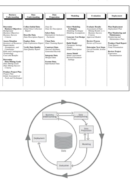
The research framework used in this study is the Cross Industry Standard Process for Data Mining (CRISP-DM). CRISP-DM is a data mining model summarizing all important steps undertaken in a data mining project. It provides a structured ap-proach to the planning and conduction of a data mining project. Being first presented and published in 1999 (Chapman, 1999) it remains one of the standard models to-day (Piatetsky-Shapiro, 2014). The model splits the data mining process into six phases, as shown in Figure 3.1. The order of steps is arbitrary and largely depen-dent on the outcome of the previous step. The arrows in the diagram describe the strongest relationships. The outer circle stands for the cyclic nature of data mining tasks: Learned lessons and solutions from a data mining project often lead to new business questions and trigger a new process (Chapman et al., 2000). The six dif-ferent steps are explained below. A more detailed overview of the six stages can be seen in Table 3.1.

1 Business understanding: This phase considers project objectives from a business perspective. Generated insights are transformed into a data mining problem definition.

2 Data understanding: During the data understanding phase, data is initially collected and analyzed to generate first insights and for accomplishing famil-iarity with the data.

3 Data preparation: This phase entails all of the steps undertaken to generate the final dataset of variables from the initial raw data, which will serve as input to the modeling tools.

4 Modeling: In the modeling phase, modeling techniques are applied. This in-volves both model selection and further fine-tuning of the models’ parameters. Since several techniques exist for modeling the same data mining problem various models can be considered.

5 Evaluation: After implementation, the models’ performance has to be evalu-ated and compared. It is important to assess whether the goals, defined during the business understanding phase, are met.

6 Deployment: In order to actually benefit from the model it needs to be de-ployed. This requires for the model to be integrated in live systems and fed with live data, in order to make valuable predictions.

These six stages provide a guideline to the research at hand: Business understand-ing was established through the background information on customer classification

in the e-commerce context in the introductory Chapter 1. This resulted in a data mining problem definition formulated as a research question in Section 1.2. Further, understanding of the actual prediction task was provided in the literature review on classification and machine learning algorithms in Chapter 2. A description of the data and a first insight leading to Data understanding will take place in Chapter 4.

Chapter 4 also includesData preparationin terms of data pre-processing as well as

feature engineering and selection. Modeling, including hyper-parameter tuning and

training, is described in the implementation Chapter 5. Evaluation and comparison

of the different algorithms are performed in Chapter 6. TheDeployment step is out

of scope for this research, since it only focuses on comparing different algorithms in respect to the already implemented and deployed baseline model, as described in Section 1.2.

3.2 Evaluation metrics

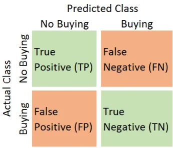
Figure 3.2: Confusion matrix, showing true positives, true negatives, false positives and false negatives.

Performance measures

Various measures exist to assess and compare the performance of machine learn-ing models on a binary classification task. These metrics are based on the so-called confusion matrix, Figure 3.2, from which one can derive the correctly pre-dicted cases, indicated in green, called true positives and true negatives. These are the cases where a visitor did not purchase anything and a no buying session was predicted and sessions where a purchase occurred and was also predicted. Also, the wrongly predicted cases can be identified, as indicated in orange, the false neg-atives, and the false positives, where a purchase occurred but none was predicted or where no purchase occurred but one was predicted.

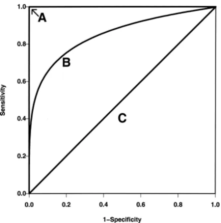
recall, also called sensitivity, is the number of true positives divided by all positives in the data set, see Equation 3.4. In the F1-score both recall and precision are con-sidered equally as shown in Equation 3.5. (Manning, Raghavan, & Schuetze, 2008). Another very important measure is the specificity which stands in contrast to the sensitivity and measures the proportion of negatives that are correctly identified as such (Equation 3.6). The trade-off between these two can be modeled through the ROC AUC, which displays the effect of different thresholds on the two metrics. The ROC AUC score is, therefore, threshold-independent. An example of ROC curves is displayed in Figure 3.3. The straight line C displays a ROC AUC of 0.5 which cor-responds to the probability of guessing and line A shows a perfect prediction with a ROC AUC value of 1. Line B shows a regular ROC curve with a value of 0.85, which approaches line A as predictions get better (Zou, OMalley, & Mauri, 2007). Most of the reviewed papers use accuracy and the ROC AUC as the performance indicator, since it provides a possibility to consider sensitivity and specificity and to nicely plot their dependency without worrying about the chosen threshold (Castanedo et al., 2014; Lo et al., 2014; Lang & Rettenmeier, 2017; Zhang et al., 2014).

Accuracy = N umber of correct predictions

T otal number of predictions =

T P +T N

T P +F P +F N+T N (3.1)

Error rate= N umber of wrong predictions

T otalnumber of predictions =

F P +F N

T P +F P +F N +T N (3.2)

P recision= N umber of true positives

T otal number of positive predictions =

T P

F P +T P (3.3)

Recall = N umber of true positives

F alse negatives+N umber of true positives =

T P

F P +T P (3.4)

F1Score=

2

1

Recall +

1

P recision

= _{F N+T P} 2

T P +

F P+T P T P

(3.5)

Specif icity = T rue negatives

T rue negatives+F alse positives =

T N

T N +F P (3.6)

Figure 3.3: Three different ROC curves. A being the perfect curve, B a regular curve and C displaying the chance of guessing. Retrieved from Zou et al. (2007).

both the performance of specificity and recall. To make the results of all algorithms comparable it is important to use the same input data for each. Further, the clas-sification threshold should be the same across all algorithms, in this case, it was decided to be set to 0.5. Lastly, to establish which algorithm performs best on which datatype the algorithms will be tested on three different datasets: The customer dataset, only compromising static customer data, the sequence dataset, containing time-depended clickstream data and static session information and the complete dataset consisting of the combined data.

Latency

Comprehensibility

Next, to those different measurements, the models will be compared based on com-prehensibility. As machine learning is applied in our everyday lives the demand for understanding the predictions is growing (Ribeiro, Singh, & Guestrin, 2016). With the General Data Protection Regulation law, taking effect in the European Union in 2018, users will even have the ’right for explanation’, offering users the possibility to request explanations about algorithmic decisions (Goodman & Flaxman, 2016). Comprehensibility is, therefore, becoming very important. Since comprehensibility can be difficult to define and is very subjective it is not considered to be the main evaluation metric.

3.3 Tool selection

clothing retailer. The software that records the data, was developed in-house and stores the interactions of visitors with the web shop in high detail. This is in line with the definition of Dumais, Jeffries, Russell, Tang, and Teevan (2014) describing click-stream data as records that store user interactions with an application in a highly detailed manner. Further, a first data analysis is conducted to facilitate data under-standing. The chapter concludes with the feature engineering as well as feature selection process.

4.1 Data description

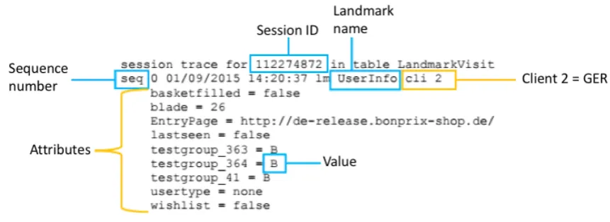
Session data exists for each web shop session of a visitor. Such a session is defined as one visit to the web shop that times out after one hour of inactivity, then a new session starts. This approach of splitting interactions into sessions is a validated approach called gap sessions, described by Chen, Fu, and Tong (2004). Throughout literature, a 30-minute gap is more common (Chen et al., 2004; Stevanovic, Vlajic, & An, 2011; Suchacka & Chodak, 2016). To identify sessions, a cookie-based ID is generated, which changes after one hour of inactivity. Each session is split into a sequence of interactions with the web shop called landmark. A landmark always consists of at least the following structure:

landmark = attribute/value

where a landmark can take n different attributes with n different values. All attributes and values of a landmark belong to the same sequence number with the same timestamp to record different informations about one event. A new landmark is written every time an interaction with the web shop occurs or the web shop renders an action. The goal is to calculate the buying probability each time a new page

Figure 4.1: Example of a Landmark, with sequence 0, session ID 112274872, name UserInfo and some attributes with different values.

is opened or an item is added to the shopping basket and to then save it as an additional attribute of the current landmark, based on which business decisions, such as displaying gift cards, can be carried out. An example of a landmark can be seen in Figure 4.1. All landmarks are stored with a session ID, a timestamp, a sequence number, their name, attributes and values in a database. For training and testing the models, only the landmarks that described the customer, the session or customer interactions were kept, such as navigating to a page and adding something to the shopping basket, to reduce the size of the dataset.

Customer data only exists if the visitor could be identified. This means if a visitor actively logged in or was automatically logged in due to restoring a cookie. If the visitor is identified various data exists to describe the customer, such as the gender, the age, the postal code as well as purchase and activity history. All of this data is anonymous and does not allow for matching it to a certain person.

4.2 Data pre-processing

The models will be trained with session and customer data of the week from 31.07.2016 until 07.08.2016 since this data was used to train the baseline model and the same data should be used for all algorithms to facilitate a comparison as mentioned in the evaluation section in Chapter 3. Data was transformed such that each visitor action within a session was written to one row of the database.

mans, it is most likely that the page was opened accidentally (e.g. if the tab was still opened on a smart-phone and appeared accidentally when the web browser was accessed). These cases are also not relevant for the use case; therefore, they can be removed along with the traffic caused by bots. Also, all traffic generated by em-ployees caused by testing and development of the web shop, was removed prior to further data pre-processing steps. These cases are marked by specific landmarks that either indicate testing or deployment and can therefore easily be removed.

Figure 4.2: The influence of the weekday on the buying and no buying decision.

4.3 Data understanding

To generate a first understanding of both the sequence as well as the customer data a first exploratory data analysis based on Excel was conducted.

4.3.1 Sequence dataset

To provide a first insight into the sequence dataset, sequence data was chosen that remains constant throughout a session. These categorical data columns are week-day, device and entry channel. All of these variables were plotted in relation to the total number of buying and no buying sessions as well as in relation to the percent-age of buying sessions out of all sessions. Buying and no buying were chosen since they are the two levels of the target variable. Therefore, the two plots both give an impression on how different variables influence the target variable of the prediction problem at hand.

Figure 4.3: The influence of the entry channel on the buying and no buying decision.

Figure 4.3 shows the influence of the different entry channels on the buying versus no buying decision. To understand the graph better the different channels are explained below.

• AFF:Affiliate marketing, such as discounts or gift cards provided by third party websites

• MAIL:The e-mail channel, such as newsletters, service letters, etc. • POR:Banner advertisement on websites

• PSM:Price search engine, a search engine that looks for the lowest prices • RET:Retargeting, personal advertisement on third party pages

• SEM:Search engine advertisement, such as Google advertisements

• SEM BR:Search engine advertisement brand specific, such as Google adver-tisements that are a result of a specific brand search

• SEO:Search engine optimization, meaning a web search engine’s unpaid re-sults

• SEO BR: Search engine optimization brand specific, meaning a web search engine’s unpaid results specific to a brand name

• SMA:Social media advertisement, such as advertisements on facebook • OTHERS:Mainly entering the website directly, via entering the URL or

Figure 4.4: The influence of the device on the buying and no buying decision.

One can clearly see from the bars in Figure 4.3 that the MAIL, OTHERS and SEM BR channel are the most used channels to enter the web shop. The large amount of sessions being entered through the OTHERS channel might be caused by the fact that under the keyword OTHERS a lot of channels are combined. The OTHERS channel also compromises a large number of cases where the web shop URL was entered directly into the browser. The high traffic through the OTHERS channel can therefore also be explained by the high number of catalog subscribers that manually enter the web shop URL in the browser after the catalog raised their interest. Looking at the line chart showing the buying percentage in Figure 4.3, one can see that AFF results in the highest percentage of buying sessions. This very high number is most likely due to the fact, that affiliate marketing entails gift cards and discounts, which result in more buying sessions. AFF is followed by MAIL, SEO BR, SEM BR and the OTHERS channel. SEM BR and SEO BR result probably in a higher buying ratio compared to SEM and SEO since the visitor was directed towards this specific online shop and not only towards an article that can be found in many other online shops.

possi-Figure 4.5: The influence of the customer identification on the buying and no buying decision.

bly due to the fact that the size facilitates the input of login and payment information. Lastly, to analyze which effect the identification of the visitor during the web shop session had on the buying decision, the customer identification variable was plotted. Results are displayed in Figure 4.5. The bars show that the number of identified visitors is smaller than the number of unknown ones, which was expected. It can also be seen that identified visitors buy more often and abort the shopping process less compared to the unknown visitors. The line chart displays that the percentage of buying sessions is more than 15 percent higher with known visitors than with unknown ones. The results indicate that the information whether the visitor could be identified or not can enhance predictive performance since the two different levels of the variable influence the buying decision differently.

4.3.2 Customer dataset

As a next step, some variables from the customer dataset were analyzed in the same fashion, to generate an understanding of the customer data. For analysis, the variables age, gender, and last device were chosen. They can be best plotted since they do not take too many different values. Gender and device are categorical variables and age takes values between 18 and 88.

Figure 4.6: Figure (a) and (b) showing the influence of the last device on the buying

and no buying decision.

Figure 4.7: The influence of the gender on the buying and no buying decision.

the prediction task.

In Figure 4.7 the influence of the gender on the buying decision is displayed. From the bars in Figure 4.7, one can clearly see that more women visit the web shop than men. The total number of women is about ten times higher than the total number of men, also the number of buying and no buying sessions conducted by women is around ten times as high as the one of men. Looking at the buying per-centage, displayed as the line in Figure 4.7, one can see that the percentages differ by less than three percentage points. The buying percentage of men is only slightly higher than the one of women, 32.5 compared to 35 respectively. This variable does therefore also not offer a lot of predictive power about the buying decision.

Figure 4.8: The influence of the age on the buying and no buying decision.

around 40 years the number of customers slightly drops, resulting in a binomial distribution with peaks at 26 and 52. For customers younger than 26 the number of customers decreases as the age decreases, analogously for people older than 52 the number of customers decreases as the age increases. The small rise for people around 80, results from aggregating all visits for ages older than 80, a so-called boundary effect. The buying and no buying behavior follows a similar curve as the total number of visitors. This relationship becomes clearer from the plotted line, displaying the buying percentage. The ratio of buying sessions is around 30% for all ages, only between the ages 33 and 57 the ratio rises to around 35%. The fact that the ages do not largely seem to differ in their buying and no buying behavior, especially regarding the ages that occur the most, results in the age variable not having a high predictive power.

In general, looking at the customer features, the data suggests that it is of high importance to the purchase prediction whether a visitor could be identified or not. The specific customer attributes themselves do not add a lot of information and are therefore not very influential on the purchase decision.

4.4 Features

4.4.1 Feature engineering

Feature engineering is the process of using domain knowledge and expertise to extract features from data that represent the underlying problem to be used as input for machine learning models. It is a not well-defined process, nevertheless, it is one of the most important steps in the development of a machine learning model. No matter how good the model is, it will not be able to predict correctly if the input features are not representative of the task. Feature engineering can be problematic since engineered features are often over-specified and incomplete (Castanedo et al., 2014).

In this study, 28 features were retrieved from the clickstream data to capture session characteristics and 20 features from the customer data to describe the cus-tomer. All of the 48 features, split by sequence and customer features, can be seen in Table 4.1. The table shows feature names, a short explanation, the data type and whether a feature can be nullable. It is further indicated which features remain con-stant throughout a whole session. Values for features that are not concon-stant, always describe events that occurred in the previous step. The green variable is the target variable, it, therefore, does not belong to the feature set.

Table 4.2: RNN features, with name, description, value and whether it can be not defined. A feature with * remains constant throughout a session. The green feature is the target variable. Customer data corresponds to cus-tomer data in Table 4.1

.

the ones used in the other feature set. Next to engineering the features, the dataset also requires further processing to make it suitable as input for the machine learning models. All algorithms, except the ones belonging to the DT category, require to re-place missing values and to encode categorical variables, which are both described in the following. Some algorithms even require further data pre-processing, these specific steps will be described in the implementation section of each algorithm.

Categorical variables

the problem of missing values is to either remove, predict or impute them. Removing records with missing values is only possible if the missing values occur completely at random (Gelman & Hill, 2016). This is not the case here since the absence of cus-tomer data does not occur randomly. Whether predicting or imputing leads to better results depends on the use case. Here imputation was chosen since it showed the best results in the paper of Hop (2013). For algorithms that do not require normaliza-tion of the data such as boosted trees and RFs unique value imputanormaliza-tion was chosen analogously to the paper of Hop (2013). This means replacing missing values by a value that does not occur in the dataset, in this case -100. Next to good results this method provides speed and simplicity. Unique value imputation should not be used for algorithms that require normalization of the data such as SVMs and FNNs, since the imputed values, being outliers, have a large influence on the normalization process. For these algorithms, missing values were imputed with the mean values of the corresponding features. Hence, a mean value imputation was performed.

4.4.2 Feature selection

Feature selection is the process of retrieving a subset of relevant features from the before engineered features. The aim is to remove redundant or irrelevant features to simplify the model, shorten training times, and reduce dimensionality and the chance of over-fitting (James, Witten, Hastie, & Tibshirani, 2013).

Figure 4.9: Importance of the 43 selected features as shown by the boosted tree baseline model. Customer features are marked in yellow font and ses-sion features in black.

of variable importance. The 43 final features were inputted into the already existing boosted tree model and variable importance was assessed. Results are shown in Figure 4.9. It can be seen that certain features are by far more important than oth-ers. Most important is the session feature avg adaP, which is the average price of

all viewed articles. Aktion(the type of interaction) andbestellkarte (if an order form

This section describes the implementation as well as hyper-parameter tuning for all implemented algorithms. Hyper-parameter tuning is only conducted on the complete dataset, since it is the dataset that, based on literature, is expected to yield the best results. Running hyper-parameter tuning on all datasets was impossible due to time and computational constraints.

Boosted Tree

The boosted tree was built analogously to the already implemented boosted tree model since it is the baseline to which other algorithms will be compared. The already used model was built in R, a programming language used for statistical computing and graphics (R: The R Project for Statistical Computing, 2017). Since

all other algorithms will be built in Python it was decided to rebuild the baseline model, to ensure that performance differences are not due to used software and libraries, but to actual differences of the algorithms. The original model was built with the XGBoost library for R, which is a gradient boosting framework including a linear model and a tree learning algorithm (XGBoost R Tutorial, 2016). Fortunately,

the same algorithm exists in Python (Scalable and flexible gradient boosting, 2016).

The model could therefore simply be transferred to the new programming language. Hyper-parameter tuning was already done when the algorithm was first engineered through grid search. These same parameter settings were used in Python and are explained below. As already mentioned in the literature research, boosted trees have the advantage of not requiring too much hyper-parameter tuning.

• max depth = 12: Describes the maximum depth of a tree, which is used to

control over-fitting, since higher depths will result in learning very specific rela-tionships (Jain, 2016).

• learning rate = 0.2: Describes the learning rate of the model. It leads to an increased robustness by shrinking the weights in each step (Jain, 2016).

• min child weight = 100: Defines the required minimum sum of weights of observations in a child node. It is useful to control over-fitting and under-fitting. Higher values prevent the model from learning too specific relationships, whereas too high values could result in under-fitting (Jain, 2016).

• num rounds = 400: Number of learning iterations carried out by the algorithm. A larger number results in a better performance while increasing training times.

All other tunable parameters were set to their default settings. For completion, the Python code of setting the hyper-parameters can be found in Appendix A Figure A.1.

Random Forest

To build the RF the implementation of the scikitlearn library RandomForestClassi-fier was used (RandomForestClassifier, 2017). Since RFs are not very prone to

over-fitting, (Breiman, 2001) they do not require a lot of hyper-parameter tuning. Mainly, there are three different parameters influencing prediction performance:

• max features: Describes the maximum number of features the algorithm tries for an individual tree. Generally, a higher number of features increases per-formance since the number of options at each node is increased. However, this does not necessarily hold true since an increase in features will also lead to a higher correlation of the individual trees (Srivastava, 2015). According to Geurts, Ernst, and Wehenkel (2016) a good solution for classification prob-lems lies around the square root of the number of features. However, to find the most optimal solution each case has to be tested.

• min samples leaf: Meaning the minimum amount of samples in the end nodes of the tree, where a smaller leaf size can lead to the effect of capturing more noise in the data.

Figure 5.1: ROC AUC results of the grid search for the parameters max features and min samples leaf for the RF algorithm.

Support Vector Machine

The implementation of the SVM follows the main constraint that training time com-plexity is more than quadratic with the number of data samples. This results in the fact that the utilized scikitlearn implementation of the algorithm does not scale well to datasets with more than a couple of 10,000 samples (SVC, 2017). It was decided

to use 100,000 data samples to train the algorithm since it was the highest number of samples still leading to reasonable training times. The input data needed to be scaled to values ranging from 0 to 1. Since SVMs are prone to misclassifying the minority class in unbalanced datasets (Liu, An, & Huang, 2006) and only a subset of the data was used to train the SVM anyways, the subset was sampled such that buying and no buying sessions were equally present.

The effectiveness of an SVM depends on the used kernel, its parameters, and the soft margin parameter C. Hsu et al. (2003) suggest to use the RGB kernel. This kernel only has one kernel parameter, namely γ. The according formula can be found in Chapter 2 in Section 2.2.2. This, therefore, leaves C and γ for hyper-parameter tuning, which was again accomplished by grid search. Values forγ were 0.0001, 0.001, 0.01 and 0.1 and C was tested with values 0.0001, 0.001, 0.01 0.1 and 1. The results in Figure 5.2 show that the highest value was obtained with aC value of 1 and aγ of 0.1. In general, the configurations with aC value of 1 resulted in the highest ROC AUC score, the smallerC got the further the score decreased. For the final implementation C of 1 and γ of 0.1 were chosen. For completion, the Python code for setting the SVM hyper-parameters can be found in Appendix A in Figure A.3.

Feed-forward Neural Network

For building the FNN the Sequential model implementation of Keras was used (The sequential model API, n.d.). This implementation provides a framework, which

leaves the possibility for intensive hyper-parameter tuning. Hyper-parameters used in FNNs can be split into two categories, determining the training and the structure of the network. Important training parameters are the loss function, the number of epochs and the batch size. The loss function compares the network’s output against the intended ground truth output (Neural Network Hyperparameters, 2015). Here,

Figure 5.2: ROC AUC results of the grid search for the parametersCandγ.

too high numbers in over-fitting. After testing various configurations the number of epochs was set to 50 since for higher numbers the prediction performance on the test dataset decreased again. Lastly, since, due to memory constraints, not all data can be passed through the network at once, a batch size has to be chosen. If mul-tiple data points are passed to the network, the average of all resulting gradients is used for updating. This yields the advantage of not capturing as much noise as updating for every single data point. The FNN was tested with different batch sizes where a batch size of 1012 yielded the best results and was still computationally fea-sible. Hyper-parameters regarding the structure of the FNN are concerned with the size and non-linearity of each layer as well as the total amount and configuration of different layers. Tuning these parameters results in too many different configurations for conducting a grid search. Therefore, a coordinate descent was used, where only one parameter is adjusted at a time to reduce the validation error (Neural Network Hyperparameters, 2015). This resulted in a final architecture with five dense

lay-ers of sizes 700, 350, 200, 64 and 1 separated by three dropout laylay-ers, to reduce over-fitting. The complete architecture in Python code can be found in Figure A.5 in Appendix A.5.

Logistic Regression