University of Warwick institutional repository: http://go.warwick.ac.uk/wrap
This paper is made available online in accordance with
publisher policies. Please scroll down to view the document
itself. Please refer to the repository record for this item and our
policy information available from the repository home page for
further information.
To see the final version of this paper please visit the publisher’s website.
Access to the published version may require a subscription.
Author(s): A. M. de Roos, O. Diekmann, P. Getto and M. A. Kirkilionis
Article Title: Numerical Equilibrium Analysis for Structured Consumer
Resource Models
Year of publication: 2010
Link to published version:
http://dx.doi.org/10.1007/s11538-009-9445-3
DOI 10.1007/s11538-009-9445-3 O R I G I N A L A RT I C L E
Numerical Equilibrium Analysis for Structured Consumer
Resource Models
A.M. de Roos
a, O. Diekmann
b, P. Getto
c,∗, M.A. Kirkilionis
daInstitute for Biodiversity and Ecosystem Dynamics (IBED), University of Amsterdam,
P.O. Box 94084, 1090GB Amsterdam, The Netherlands
b
Department of Mathematics, University of Utrecht, Budapestlaan 6, P.O. Box 80010, 3508 TA Utrecht, The Netherlands
c
BCAM—Basque Center for Applied Mathematics, Bizkaia Technology Park, 48160 Derio, Bizkaia, Spain
d
Department of Mathematics, University of Warwick, CV4 7AL Coventry, UK
Received: 3 March 2009 / Accepted: 16 July 2009 / Published online: 31 July 2009 © The Author(s) 2009. This article is published with open access at Springerlink.com
Abstract In this paper, we present methods for a numerical equilibrium and stability analysis for models of a size structured population competing for an unstructured re-source. We concentrate on cases where two model parameters are free, and thus existence boundaries for equilibria and stability boundaries can be defined in the (two-parameter) plane. We numerically trace these implicitly defined curves using alternatingly tangent prediction and Newton correction. Evaluation of the maps defining the curves involves in-tegration over individual size and individual survival probability (and their derivatives) as functions of individual age. Such ingredients are often defined as solutions of ODE, i.e., in general only implicitly. In our case, the right-hand sides of these ODE feature discon-tinuities that are caused by an abrupt change of behavior at the size where juveniles are assumed to turn adult. So, we combine the numerical solution of these ODE with curve tracing methods. We have implemented the algorithms for “Daphnia consuming algae” models in C-code. The results obtained by way of this implementation are shown in the form of graphs.
Keywords Numerical equilibrium analysis·Structured populations·Stability
boundaries·Hopf bifurcation·Consumer resource models·Delay equations·Renewal equations·Delay differential equations·Daphnia models
1. Introduction
In this paper, we present methods for a numerical equilibrium and stability analysis of a class of models of the interaction between a structured consumer population and an unstructured resource population.
∗Corresponding author.
In unstructured consumer resource models and in predator prey models, one typically finds a Hopf-bifurcation marking the destabilization of an interior equilibrium and the emergence of a stable limit cycle (Rosenzweig,1971). In de Roos et al. (1990), one finds a model of a size structured population of Daphnia magna consuming algae, which is pa-rameterized on the basis of experimental data. Based on extensive numerical calculations, it is concluded in de Roos et al. (1990) that incorporating size structure of the consumer induces additional features, namely the possibility of the coexistence of a stable and an unstable limit cycle and even the coexistence of two stable limit cycles.
In Diekmann et al. (2007), a theoretical framework is described that establishes exis-tence and uniqueness, the principle of linearized stability and the Hopf-bifurcation the-orem for a class of abstract integral equations. For given resource, the dynamics of a structured population can be described by a renewal equation; see Metz and Diekmann (1986). This equation can also be classified as a Volterra integral equation or a functional equation of delay type (with continuously distributed delay); see Diekmann et al. (1995). Incorporating competition then amounts to adding an equation for the resource dynam-ics (Diekmann et al.,2007). This equation has on the right-hand side a similar structure as the renewal equation, but the left-hand side consists of the time derivative of the un-known resource concentration, whereas in the case of the renewal equation, it consists of the unknown function itself. It hence should be called an integro-differential equation or a delay differential equation (again with continuously distributed delay). Hence, in sum-mary, we shall speak of a system of delay equations, a renewal equation coupled to a delay differential equation. Such systems are equivalent to special cases of the mentioned abstract integral equations; see again (Diekmann et al.,2007). In de Roos et al. (2009), the mathematical setting of Diekmann et al. (2007) is used to establish an analytical stability and bifurcation theory for structured consumer resource models with special attention for the Daphnia model in de Roos et al. (1990). Our aim here is to complement the analyti-cal theory in de Roos et al. (2009) with tools for the numerical equilibrium and stability analysis of such models. Even though we use Daphnia models to test our algorithms, our approach works for more general structured consumer resource models. Moreover, we use formulations that should be easy to generalize to other structured population models.
As key results of the analysis of qualitative behavior, in de Roos et al. (1990) curves in two-parameter space marking stability boundaries where Hopf-bifurcations occur were presented. Integrals, which arise naturally when modeling structured populations, could in the case of the Daphnia model be evaluated analytically, and thus the curves could be approximated by coding established predictor- corrector methods (Allgower and Georg, 1990) without it being necessary to refer to numerical integration. We present a method here to compute stability boundaries for models specified in terms of general vital rates. Integrals involving these general vital rates can be evaluated by integration of a system of coupled ODE, which is generally not possible by hand. The idea, which can be found al-ready in Kirkilionis et al. (2001), is to combine the curve tracing methods with numerical integration of the ODE. We use this idea here to establish methods to compute existence and stability boundaries for structured consumer resource models formulated as systems of delay equations.
Much of the length of this paper is caused by the complexity of the characteristic equation. This complexity is due to the fact that the following issues are involved in its computation:
– differentiation of solutions of ODE with respect to infinite dimensional parameters, – discontinuities at the size where adulthood is reached,
– the rewriting of ingredients of the characteristic equation as solutions of (real) ODE.
In de Roos et al. (2009), an expression for the ingredients of the characteristic equation for our class of structured consumer resource models is given. Our present derivation of the characteristic equation is much inspired by this paper, but we found that for the numer-ical computation of the elements a different representation of the characteristic equation is more convenient.
In Section2, we introduce the analytic setting for a class of models describing the interaction of a structured consumer population with an unstructured resource popula-tion. We formulate the population equations and discuss the existence of a unique in-terior equilibrium. Then we concentrate on the case where two model parameters are free and define existence boundaries for the equilibrium in the (two-parameter) plane. In this plane, we then define a curve marking Hopf-bifurcation points. The main ingredi-ent here is the characteristic equation obtained via linearization of the population equa-tions.
In Section3, we present methods to numerically approximate the curves defined in Section2. We start with an algorithm for the numerical integration involved in the approx-imation of equilibria. In a further algorithm, we show how to achieve this approxapprox-imation by a combination of the numerical integration method and a Newton-method. In the case of two free parameters, we show how the curves can be continued by combining first tangent prediction and then correction with a Newton method with numerical integration. Here, the map defining stability boundaries is much more involved than the one defin-ing existence boundaries, due to the already mentioned complexity of the characteristic equation.
2. Consumer resource dynamics
We present the analytic formulation of the class of models here that we will investigate. We first give the population equations and equilibrium conditions. Then we define ex-istence and stability boundaries in two parameter planes. Much of Sections2.1and2.2 overlap with de Roos et al. (2009) and is presented here for the sake of completeness.
2.1. The model
We first derive the population equations—stepping from the individual level to the pop-ulation level—formally, i.e., we postpone smoothness discussions. We then give smooth-ness assumptions, discuss discontinuities induced by an abrupt onset of reproduction, and finally become more specific about the derivation of size and survival as functions of age.
2.1.1. The population equations formally
Let us denote byS(t ) the available resource or food concentration at timet. Our way of bookkeeping at the population level leads us to introduce histories, first as functions defined on(−∞,0]. For the resourceS,we introduce the notation
St(σ ):=S(t+σ ), σ∈(−∞,0], (1)
which is common in the theory of functional differential equations (Hale,1977). ThenSt is a history for everyt, the history of the resource at timet.
Let us assume that there is only one possible size xbat which individuals are born. Next, we introduceX(a, Ψ )as the size that an individual has at agea, given that it has experienced historyΨ in the time interval[−a,0]. ThenX(a, St)is the size that an in-dividual has at ageaand timet, given that it has experienced resource concentrationS
in the time interval[t−a, t]; see Fig.1. Likewise, we introduceF(a, Ψ )as the survival
probability to ageaof an individual, given that if it survives, it has experienced historyΨ
in the time interval[−a,0]. ThenF(a, St)is the probability for an individual to reach age
aat timetgiven that it experiences resource concentrationSin the time interval[t−a, t]. Next, we denote byβ(x, y)the rate of reproduction of an individual of sizexunder re-source conditionyand byγ (x, y)the rate of food consumption of an individual of sizex
under resource conditiony. So, for example,β(X(a, St), S(t ))is the rate of reproduction of an individual of agea at timet. Finally,f (y)denotes the intrinsic rate of change of the resource, meaning the rate of change in absence of the consumer. Let us denote by
b(t )the population birth rate, i.e., the number of individuals born (in total or per unit of area or volume, depending on the context) with sizexbper unit of time at timet. Let us denote byh >0 the maximum lifetime of an individual under ideal food conditions. Then we can describe the population dynamics by the system of equations
b(t )= h
0
βX(a, St), S(t )
F(a, St)b(t−a) da, (2)
S(t )=fS(t )− h
0
γX(a, St), S(t )
F(a, St)b(t−a) da; (3)
Fig. 1 Equation (2): reproduction at timetas induced by the history of resource and population birth rate.
2.1.2. Smoothness conditions and discontinuities caused by abrupt onset of reproduction
Motivated by the “Daphnia consuming algae” model in de Roos et al. (1990), we suppose that at size xA> xb juveniles mature. Keeping in mind that we would like to linearize later, we should formalize the assumption that rates are smooth, except for a possible jump inxA. We thus assume thatβandγ can be defined on[xb,∞)via functions that areC1on [xb, xA] ×R+and on[xA,∞)×R+. This leads to unique definitions on[xb,∞)\{xA} × R+and to a double definition in(xA, y)for ally∈R+. This double definition, however, is irrelevant, as we are ultimately interested in the integrated functions. Finally, we assume thatβ(x, y)=0 for allx∈ [xb, xA)and ally. So, neither forβ, nor forγ there can be expected continuity, let alone differentiability, inxA. Next, suppose thatf:R+−→Ris
C1. We assume thatSis continuous and restrict the domain of definition of histories, in particular ofSt, from(−∞,0]to[−h,0]. To guarantee integrability in (2)–(3) and for later differentiability in theS-component, we require thatXandFare such that
C[−h,0],R−→L∞[0, h],R,
ψ−→X(·, ψ ), (4)
ψ−→F(·, ψ )
are continuously differentiable maps. Next, if an individual matures exactly at the present time for a given food historyψ, we denote its age at maturation byaA, i.e., we defineaA via the equation
the solvability of which will be discussed in Section2.1.3below. Finally, we assume that
bis nonnegative and integrable. The population equations, reflecting the jump inxAare now given by
b(t )= h
aA(St)
βX(a, St), S(t )
F(a, St)b(t−a) da, (6)
S(t )=fS(t )− aA(St)
0
γX(a, St), S(t )
F(a, St)b(t−a) da
−
h
aA(St)
γX(a, St), S(t )
F(a, St)b(t−a) da, (7)
where the integrals fromaA(St)tohshould be interpreted as zero whenaA(St)≥h. In (7), we have split the integration interval into two parts in order to highlight the discontinuity in the integrand. In the following, however, we shall simply write one integral from zero toh, as the jump discontinuity is harmless with respect to integration.
2.1.3. Computation of size and survival functions as solutions of ODE
We show howXand F can be computed for the case that one has given ratesg(x, y)
and μ(x, y) of individual growth and mortality. Just like forγ, we also assume that
g, μ:R2
+−→R+are C1 on[xb, xA] ×R+and on [xA,∞)×R+. We additionally as-sume the existence of positive lower bounds forg andμthat are uniform for all sizes and uniform for all resource conditions outside a neighborhood of zero which should be chosen sufficiently small not to contain positive equilibria (which will be defined below). The definition ofXand F in terms of the history of a time dependent resource via the ratesgandμleads to a certain notational complexity. We here use the same notation as in de Roos et al. (2009). We denote byx(α)=x(α;a, ψ )the size of an individual at ageα, given that at agea, if still alive, it has experienced resource historyψ. Likewise, we denote byF˜(α)= ˜F(α;a, ψ )the probability that an individual survives up to ageα, given that at agea, if still alive, it has experienced resource historyψ. Then we can define
X(a, St):=x(a;a, St) and F(a, St):= ˜F(a;a, St).
We compute x(α) and F˜(α) by solving the system of (one-sidedly) coupled nonau-tonomous ODE
x(α)=gx(α), ψ (−a+α), 0< α≤a,
(8)
x(0)=xb, ˜
F(α)= −μx(α), ψ (−a+α)F˜(α), 0< α≤a,
(9) ˜
F(0)=1.
2.2. Steady states
For the system (6)–(7), an equilibrium is a pair of constants(b, S), such that (b, S):= (b, S) fulfills (6)–(7). Ifb=0,S should be such thatf (S)=0. In this case, we have a trivial equilibrium(0, S), which we disregard here. A nontrivial equilibrium is given by a pair of constants(b, S)fulfilling
R0
S−1=0, (10)
fS−ΘSb=0, (11)
R0
S:=
h
τ
βXa, S, SFa, Sda,
(12)
ΘS:= h
0
γXa, S, SFa, Sda,
where we denote by
τ:=aA
S
the age at which individuals mature under steady state conditions. Note thatR0(S)and
Θ(S)are, respectively, the expected lifetime offspring production and the expected life-time resource consumption of a consumer individual, which gives obvious interpretations of the steady state conditions. As, forΘ(S) >0, (11) can be solved explicitly with respect tob, we write
bS:= f (S)
Θ(S), (13)
and reduce the steady state problem to finding anSsatisfying (10). A typical case is that (10) has a unique solution; see, e.g., de Roos et al. (1990), and also here we assume that this holds. We give a method to approximate the solutionSof (10) in Section3.2.
2.2.1. Existence boundaries
We suppose in the following that two model parameters, which we denote byα1andα2, are free. We will or will not incorporate (free) parameter dependence of functions into the notation according to convenience and relevance in the context. We then rewrite (10)–(11) as
R0
α1, α2, S
−1=0, (14)
b:=f (α1, α2, S) Θ(α1, α2, S)
, (15)
(where it will prove convenient in Section 3 to denote first parameters and then the equilibrium). The bcomponent of the equilibrium becomes positive if the curve in the
α1–α2-plane defined by the two equations
fα1, α2, S
and (14) is crossed in the appropriate sense. We hence call this curve the existence bound-ary for the nontrivial equilibrium.
2.2.2. Existence boundaries for Daphnia models and equilibrium curves
In the models of Daphnia consuming algae, we assume (in absence of Daphnia) chemo-stat or logistic algal dynamics and chooseα1as the mortality for Daphnia andα2as the carrying capacity for algae. Hence, typically, for givenS,f is independent ofα1andR0 independent ofα2. Moreover, (16) is equivalent toS=α2for chemostat or to “S=0 or
S=α2” for logistic dynamics; see Section4below. Finally, typically (14) has no solution forS=0, as in the absence of food there is no reproduction. In summary, for Daphnia, the existence boundary defined by (14) and (16) can equivalently be defined by
S=α2, R0
α1, S
−1=0, (17)
where we dropped the nonmanifestingα2-dependence in the notation ofR0. It is hence clear that in this special setting the existence boundary in theα1–α2-plane and the curve describing how the equilibrium changes if one parameter varies are equal. We will give methods to compute existence boundaries for both the general setting and the setting for
Daphnia in Section3.
2.2.3. Steady state defining functions as ODE and stopping criteria for integration
As in Kirkilionis et al. (2001), in view of the interdependence of functions and the dis-continuity atxAwe propose to compute several model ingredients as solutions of ODE. We introduce two alternative criteria for ending the integration of the ODE. The choice of which one to use should depend on the biological problem one considers. The first is the reaching of a maximum ageAmax, in which case we should chooseh:=Amax. The second criterion is the one proposed in Kirkilionis et al. (2001): For everyε∈(0,1),we define
aε=aε(S)via the equationF(aε, S)=ε, i.e., as the age at which the probability that an individual survives up to it has decreased toε, and assume that the functionS→aε(S) is bounded, which is granted, ifFis defined viaμas in Section2.1.3. We callεthe
sur-vival tolerance. When using this stopping criterium, we redefinehas the supremum of the functionS→aε(S). To facilitate the exposition, we will here and in the algorithms below concentrate on the second criterion, also since we believe that it is obvious what should be changed when using the first. We have implemented both criteria and will show the results for both. We associate with the steady state conditions the system of coupled autonomous ODE
d daX
a, S=gXa, S, S, a > a0,
Xa0, S
=x0,
(18)
d daF
a, S= −μXa, S, SFa, S, a > a0,
Fa0, S
=f0,
(19)
d dar
a, S=βXa, S, SFa, S, a > a0,
ra0, S
=r0,
d daθ
a, S=γXa, S, SFa, S, a > a0,
θa0, S
=θ0.
(21)
Note thatr denotes cumulative offspring, so corresponds toR0and θ cumulative con-sumption, so corresponds toΘ. We have written the ODE for arbitrary initial data, as we would like to be able to solve the ODE for various initial data to cope with discontinuities. The natural start is witha0=0,x0=xb,f0=1,r0=0, andθ0=0.
Remark 2.1. Of courseXandFas defined by (8)–(9) equalXandFas defined by (18)– (19) only for these natural initial conditions. Since we use the two sets of ODE in different contexts, this should not lead to misunderstanding.
Then if a0=0, x0=xb, f0=1, r0=0, and θ0=0, we can integrate from zero to aA and next, with initial conditions guaranteeing continuity, from aA to h to get
R0(S)=r(h, S)andΘ(S)=θ (h, S). We therefore introduceRε(S):=r(aε, S) (consis-tent forε=0),Θε(S):=θ (aε, S)andbε(S):=Θf (S)
ε(S)as approximations forR0(S),Θ(S)
andb(S).
2.2.4. Definition of approximated existence boundaries
For general consumer resource models, the approximated existence boundary for equilib-ria is the curve defined by
Gε
α1, α2, S
=0, (22)
where
Gε
α1, α2, S
:=
Rε(α1, α2, S)−1
f (α1, α2, S)
(23)
and where Rε can be computed via integration of (18)–(20). For Daphnia models, the existence boundary can be computed by tracing the curve defined by
Gε
α1, S
=0, (24)
where
Gε
α1, S
:=Rε
α1, S
−1, (25)
and where againRεcan be computed via integration of (18)–(20).
2.3. Stability boundaries in a two parameter plane
crosses the imaginary axis (recall that non-real roots cross in complex conjugate pairs). As a first step, we thus derive the characteristic equation for (6)–(7). In the case of two free parameters, one can then define stability boundaries for equilibria inR2, interpreted asα1–α2-space, as explained below.
2.3.1. The characteristic equation
We will show in AppendixAthat if one linearizes (6)–(7) and plugs in exponential trial solutions, one gets a characteristic equation of the form
det
Mb, S, λ−
1 0
0 λ
=0, (26)
where, if one uses that (6)–(7) are linear inbfor givenS, one can show thatMis of the form
Mb, S, λ=
Ψ1(S, λ) bΨ2(S, λ)
Ψ3(S, λ) f(S)+bΨ4(S, λ)
, (27)
for functionsΨi,i=1, . . . ,4 to be specified (whereiis a super-index, not a power). The
λ-dependence inMis induced by the delay and to understand the form of the subtracted matrix recall that (2)–(3) is a renewal equation and a delay differential equation, such that theλarises through differentiation. We refer to (de Roos et al.,2009) for a representation involving Laplace transforms, which for numerical computations is less convenient. If we plug (13) into (27), we see that (26) is equivalent to
0=fS Ψ1S, λ−1Ψ4S, λ−Ψ2S, λΨ3S, λ
+ΘSΨ1S, λ−1fS−λ. (28)
2.3.2. Stability boundaries
To define stability boundaries, we should first plugλ=iω,ω≥0, into (28) and rewrite the complex equation as two real equations. To this aim, we define real functionsΨrj(S, ω),
Ψij(S, ω),j=1, . . . ,4, such that
ΨjS, iω=Ψj r
S, ω+iΨijS, ω (29)
(and where the subindicesrandi refer to “real” and “imaginary”). If we plug this into (28), a straightforward computation shows that the complex equation (28) is equivalent to the system of two real equations defined by
HS, ω=0, (30)
where
HS, ω:=fS
Ψr1S, ω−1
Ψr4(S, ω) Ψi4(S, ω)
+Ψi1S, ω
−Ψi4(S, ω) Ψr4(S, ω)
−Ψr3S, ω
Ψr2(S, ω) Ψi2(S, ω)
+Ψi3S, ω
Ψi2(S, ω)
+ΘS
fS
Ψ1
r(S, ω)−1
Ψ1
i(S, ω)
+ω
Ψ1
i(S, ω) 1−Ψ1
r(S, ω)
. (31)
If we now incorporate two parametersα1andα2into the notation, we can define a system of three real equations
Gα1, α2, S
=0,
(32)
Hα1, α2, S, ω
=0,
where
Gα1, α2, S
:=R0
α1, α2, S
−1,
in the four variablesS,ω,α1,andα2. Hence, generically (32) defines a curve that can be projected to theα1–α2-plane.
Remark 2.2. Note that forp≥2 inp-dimensional parameter space the stability boundary is of dimensionp−1. We choosep=2 for the following reasons. Forp=2, Eqs. (32) define a curve, for the numerical computation of which we can adapt established predictor-corrector algorithms. Forp=3, the equations analogous to (32) would define a surface in three- dimensional parameter space, an object much more difficult to compute numer-ically than a curve. Forp≥4, in addition to numerical difficulties that this choice would involve, the shape of the stability boundary would be hard to understand due to constraints of the human visual system.
We call the region in parameter space, where the positive equilibrium is stable, the stability region. The stability boundary is the boundary of this region. The stability region may have several components. Even if the stability region consists of one component, the boundary may consist of several connected components. We determine these compo-nents as solutions of (32) with eitherω=0 orω >0. (Note that forω=0 system (32) reduces to two equations in the three variablesS,α1,andα2, since the component ofH corresponding to the imaginary part is identically zero forω=0.)
In order that a solution of (32) corresponds to a component of the stability boundary, the number of roots of the characteristic equation in the right-half plane should be zero on one side of the curve. In the present case, there is only one curve corresponding to
ω=0 and this is the already computed existence boundary. At the existence boundary, the trivial and the nontrivial equilibrium exchange stability (we call this a “supercritical” transcritical bifurcation, in order to express that the nontrivial equilibrium is positive, and hence biologically meaningful, for parameter values for which the trivial steady state is unstable). So, from now on, we focus onω >0. Since roots occur in complex conjugate pairs, solution curves of (32) now correspond to Hopf bifurcation (if we cross the curve transversally in a regular point; note that, for instance, we may have two pairs crossing the imaginary axis in a self-intersection of the curve; see, e.g., Fig.5below).
Remark 2.3. Note that there may be other curves at which roots are on the imaginary axis
are roots in the right-half plane at both sides of the curve; see Chapter XI in Diekmann et al. (1995) (whether one speaks of one or several curves may depend on whether or not one includes the point at infinity in the parameter plane).
In Sections3.5–3.6, we give methods to trace stability boundaries numerically.
2.3.3. The entries of the characteristic matrix
We here give representations for the functions Ψi in (27). In steady state, the resource abundance is time independent and, therefore, so is the size-age relation. Since in addition the representation of theΨjis quite involved, we introduce the shorter notation
β(a):=βXa, S, S, β1(a):=
∂
∂xβ(x, S)(x,S)=(X(a,S),S),
(33)
β2(a):=
∂ ∂Sβ(x, S)
(x,S)=(X(a,S),S)
, F(a):=Fa, S
and analogously forgi,γi,andμi, wherei=1,2. It is important to keep in mind, how-ever, the dependence of functions, rates, and derivatives on the steady state conditionS, on the functionX(a, S), which is given only implicitly, and on parameters. In AppendixA, we derive (26) and from it that
Ψ1S, λ= h
τ
e−λaβ(a)F(a) da,
(34)
Ψ3S, λ= − h
0
e−λaγ (a)F(a) da,
Ψ2S, λ= h
τ
β2(a)F(a) da
+
h
τ
e−λa β(a)L(a, λ)+β
1(a)F(a)K(a, λ)
da
+
g+ g−−1
e−λτKτ , λ
h
τ
β1(σ )F(σ ) dσ
+μ−−μ+
g− K
τ , λ
h
τ
β(a)F(a)e−λada
+F(τ )β+
g− e
−λτKτ , λ, (35)
Ψ4S, λ= − h
0
γ2(a)F(a) da
−
h
0
e−λa γ (a)L(a, λ)+γ1(a)F(a)K(a, λ)
da
−
g+ g−−1
e−λτKτ , λ
h
τ
−μ−−μ+
g− K
τ , λ
h
τ
γ (a)F(a)e−λada
−F(τ )
g− γ
+−γ−e−λτKτ , λ, (36)
definingg+:=g(xA+, S),g−:=g(xA−, S)as the one-sided limits, analogously for the other rates, andKandLas the solutions of
∂
∂aK(a, λ)=g1(a)K(a, λ)+g2(a)e
λa, a > a
0,
(37)
K(a0, λ)=k0,
∂
∂aL(a, λ)= −μ(a)L(a, λ)−μ1(a)K(a, λ)F(a)−μ2(a)e
λaF(a),
a > a0, (38)
L(a0, λ)=l0
fora0:=0,k0:=0 andl0:=0.
Remark 2.4. Note that if all vital rates are additionally continuous inxA the last three terms inΨ2andΨ4equal zero (note that such a continuity assumption would imply that
β+=0), such that the situation simplifies considerably.
2.3.4. Computing entries in the characteristic matrix by solving real ODE
The definition of our curve involves the system of real equations (30) for the real func-tionsΨij,Ψrj,j=1, . . . ,4. These functions are defined via the complex functionsΨj,
j =1, . . . ,4 in (29), which are defined in (34)–(38). Moreover, the ODE-solver in our implementation requires the specification of real ODE. We therefore in the following re-defineΨij(S, ω)andΨrj(S, ω)as solutions of real ODE.
First, we plugλ=iωinto (37)–(38) and rewrite these equations as a system of ODE for real functionsKr,Ki,Lr,Li, which fulfill (when we suppress the dependence onω andSin the notation)
K(a, iω)=Kr(a)+iKi(a), L(a, iω)=Lr(a)+iLi(a). (39)
We then get
Kr(a)=g1(a)Kr(a)+g2(a)cosωa,
Ki(a)=g1(a)Ki(a)+g2(a)sinωa,
a > a0, (40)
Kr(a0)=k0r, Ki(a0)=ki0,
Lr(a)= −μ(a)Lr(a)−μ1(a)F(a)Kr(a)−μ2(a)F(a)cosωa,
Li(a)= −μ(a)Li(a)−μ1(a)F(a)Ki(a)−μ2(a)F(a)sinωa,
a > a0, (41)
To write down the real ODE to redefine (34)–(36) forλ=iωit is convenient to introduce real functions
Ke
r(a1, a2):=Re
e−iωa1K(a2, iω)=Kr(a2)cosωa1+Ki(a2)sinωa1,
Kie(a1, a2):=Im
e−iωa1K(a2, iω)=K
i(a2)cosωa1−Kr(a2)sinωa1
(42)
and analogouslyLe
r(a1, a2)andLei(a1, a2). Next, we should define real functionsψrj=
ψrj(a, S, ω)andψij=ψ j
i(a, S, ω),j=1, . . . ,4, such thatΨ j
r(S, ω)=ψrj(h, S, ω)and
Ψij(S, ω)=ψij(h, S, ω)withΨrj andΨij as in Section2.3.2. This holds if we defineψ j r andψijvia the real ODE
d daψ
1
r(a)=β(a)F(a)cosωa,
d daψ
1
i(a)= −β(a)F(a)sinωa,
ψ1
r(a0)=ψ10,r, ψi1(a0)=ψ10,i,
a > a0, (43)
d daψ
2
r(a)=β2(a)F(a)+β(a)Lre(a, a)+β1(a)F(a)Kre(a, a)
+
g+ g−−1
β1(a)F(a)Kre
τ , τ
+μ−−μ+
g− β(a)F(a)K
e r
a, τ,
d daψ
2
i(a)=β(a)L e
i(a, a)+β1(a)F(a)Kie(a, a)
+
g+ g−−1
β1(a)F(a)Kie
τ , τ
+μ−−μ+
g− β(a)F(a)K
e i
a, τ, a > a0,
ψ2
r(a0)=ψ20,r, ψi2(a0)=ψ20,i,
(44)
d daψ
3
r(a)= −γ (a)F(a)cosωa,
d daψ
3
i(a)=γ (a)F(a)sinωa,
a > a0, (45)
ψr3(a0)=ψ30,r, ψ
3
i(a0)=ψ30,i,
d daψ
4
J,r(a)= −γ2(a)F(a)−γ (a)Lre(a, a)−γ1(a)F(a)Kre(a, a),
d daψ
4
J,i(a)= −γ (a)L e
i(a, a)−γ1(a)F(a)Kie(a, a),
ψ4
J,r(a0)=ψJ,04,r, ψJ,i4 (a0)=ψJ,04,i,
d daψ
4
r(a)= −γ2(a)F(a)−γ (a)Lre(a, a)−γ1(a)F(a)Kre(a, a)
−
g+ g−−1
γ1(a)F(a)Kre
τ , τ
−μ−−μ+
g− γ (a)F(a)K
e r
a, τ,
d daψ
4
i(a)= −γ (a)Lei(a, a)−γ1(a)F(a)Kie(a, a)
−
g+ g−−1
γ1(a)F(a)Kie
τ , τ
−μ−−μ+
g− γ (a)F(a)K
e i
a, τ,
a > a0,
ψr4(a0)=ψ40,r, ψ
4
i(a0)=ψ40,i,
(47)
for appropriate initial conditions, which will be specified in Sections3.5–3.6below. The functionsψ4
J,randψJ,i4 will be used to define initial conditions forψr4andψi4ataε.
2.3.5. Definition of the approximated stability boundaries
We define the approximation ofH as
Hε
S, ω=fS
ψr1aε, S, ω
−1
ψ4
r(aε, S, ω)
ψ4
i(aε, S, ω)
+ψi1aε, S, ω
−ψ4
i(aε, S, ω)
ψ4
r(aε, S, ω)
−ψr3aε, S, ω
ψ2
r
aε, S, ω
ψi2(aε, S, ω)
+ψi3aε, S, ω
ψ2
i(aε, S, ω) −ψr2(aε, S, ω)
+ΘSfS ψ
1
r(aε, S, ω)−1
ψ1
i(aε, S, ω)
+ω
ψ1
i(aε, S, ω) 1−ψ1
r(aε, S, ω)
.(48)
Next, we incorporate dependence onα1andα2into the notation and define a map
Fε
α1, α2, S, ω
:=Gε
α1, α2, S
, Hε
α1, α2, S, ω
, (49)
where
Gε
α1, α2, S
:=Rε
α1, α2, S
−1. (50)
We can then define the approximated stability boundary by
Fε
α1, α2, S, ω
=0,
ratebεis defined as
bε
α1, α2, S
= f (α1, α2, S)
Θε(α1, α2, S)
. (51)
The functionsψrj and ψij can be computed via (41)–(47) in terms ofX andF and fi-nallyX,FandΘεare defined via (18), (19), and (21).
3. Numerical approximation techniques
We here give iterative methods to approximate solutions for the problems discussed in the last section. As in Kirkilionis et al. (2001), we present the methods in the form of algorithms in pseudo-code established in Allgower and Georg (1990). This pseudo-code is designed to be understandable independent of whether the reader is familiar with par-ticular coding languages.
3.1. Integration to compute equilibria
The following two algorithms can be used to perform the numerical integration to com-puteGεandbε for givenSand a given set of parameters. These computations are used to locate equilibria, to continue them as a function of one parameter, to compute stabil-ity boundaries, and to compute the population birth rate for any of the located equilibria. The first algorithm, i.e., the algorithm to evaluateGε(S)for givenScan also be used to test how close an initial guess is to an equilibrium point. As numerical computation of bothr(aε, S)andθ (aε, S)involves integrating (18)–(19), it may seem most efficient to integrate the four ODE (18)–(21) simultaneously. We here, however, split the integration procedures for the two ingredients for the following reason. When, e.g., searching for solutions ofR0(S)−1=0 through an iterative process, the numerical integration to com-puter(aε, S)has to be repeated for differentS, but integration of (21) is only needed for the computation ofbvia (13). Numerical integration of (21) hence only has to be carried out once with the final approximation forS. We assume that we are able to choose the survival toleranceεso small that under the relevant food conditionSindividuals reach sizexAbefore the survival probability decreases toε.
Remark 3.1. For the implementation of the algorithms, we point out that stopping ataA and ataε requires the use of a special integration method such as DOPRI5 or DOPRI8 (we have used DOPRI5) that can handle event detections; see Hairer et al. (1987).
Algorithm 3.2 (Integration to evaluateGε). input
begin
ε >0; (survival tolerance)
S; (given value)
a0:=0,x0:=xb,f0:=1;
integrate in parallel (18)–(19) untilX(a, S)=xA;
setτ:=a;
storeτandF(τ , S);
a0:=τ,x0:=xA,f0:=F(τ , S),r0:=0;
integrate in parallel (18)–(19) and (20) untilF(a, S)=ε;
aε:=a;
Gε(S):=r(aε, S)−1.
Algorithm 3.3 (Computation ofbε). input
begin
ε >0; (survival tolerance)
S; (given value)
end
a0:=0,x0:=xb,f0:=1,θ0:=0;
integrate in parallel (18)–(19) and (21) untilX(a, S)=xA;
setτ:=a;
storeτ,F(τ , S)andθ (τ , S);
a0:=τ,x0:=xA,f0:=F(τ , S),θ0:=θ (τ , S);
integrate in parallel (18)–(19) and (21) untilF(a, S)=ε;
aε:=a;
storeθ (aε, S);
computef (S);
bε:=θ (af (S)
ε,S).
3.2. Approximation of equilibria
3.2.1. Numerical differentiation
For our approximation of all partial derivatives, we use throughout two numerical con-stantsδ1andδ2,δ1> δ2>0. We then approximate the partial derivative of a functionF inxin theith component as
∂F ∂xi
x=1
δ
Fx1, . . . , xi+δ, xi+1, . . . , xN
−Fx, (52)
whereδ:=max{xiδ1, δ2}. Here, the second argument in the maximum function is used when the point to be evaluated is close to zero.
3.2.2. Broyden updates
We denote by A∗ the transpose of a matrix A and by · the Euclidean norm. Then we define the Broyden update of the Jacobian given two successive approximate solution pointsy(k),y(k+1)via
η(k):=y(k+1)−y(k), ζ(k):=Gε
y(k+1)−Gε
y(k),
and
A(k+1):=A(k)+(ζ
(k)−A(k)η(k))η(k)∗
η(k)2 . (53)
Algorithm 3.4 (Numerically solveGε(S)=0). input
begin
ε >0; (survival tolerance)
δ1, δ2; (accuracy constants for numerical differentiation)
εG, εy>0; (numerical accuracy constants)
S(0); (initial guess)
end
y(0):=S(0);
computeGε(y(0))with Algorithm3.2;
computeA(0)≈G
ε(y(0))via numerical differentiation using Algorithm3.2; solveA(0)η(0)= −G
ε(y(0))with respect toη(0);
y(1):=y(0)+η(0); (new approximation to equilibrium)
computeGε(y(1))with Algorithm3.2;
ifη(0)< ε
yandGε(y(1))< εGthenS:=y(1); (algorithm stops)
repeat (iteration loop)
k:=k+1;
compute Broyden updateA(k)withy(k),y(k−1)and (53);
solveA(k)η(k)= −G
ε(y(k))with respect toη(k);
y(k+1):=y(k)+η(k); (new approximation to equilibrium)
computeGε(y(k+1))with Algorithm3.2;
until
η(k)< εy, Gε
y(k+1)< εG;
S:=y(k+1); (new approximation accepted).
To compute an approximation of an equilibrium, it remains to combine the previous algorithm with the computation of the population birth rate via Algorithm3.3for the final value ofS.
Algorithm 3.5 (Approximation of equilibrium). input
begin
ε >0; (survival tolerance)
δ1, δ2; (accuracy constants for numerical differentiation)
εG, εy>0; (numerical accuracy constants)
S(0); (starting point, initial guess)
end
findSnumerically solvingGε(S)=0 via Algorithm3.4;
computebε(S)via Algorithm3.3;
(b, S):=(bε(S), S); (approximation of the equilibrium).
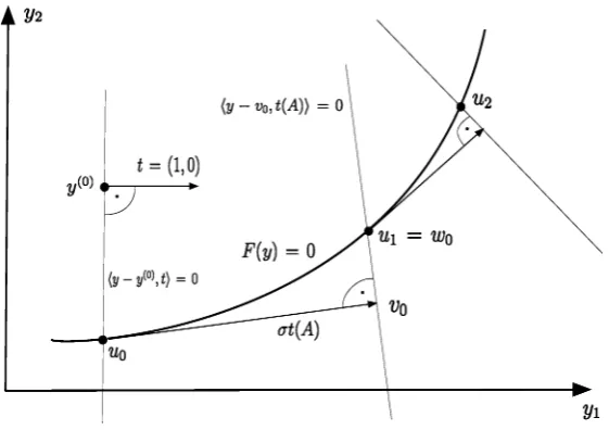
3.3. Numerical tracing of curves
We first outline the idea how to numerically trace a curve. We here use pseudo-arc length continuation as described in Kuznetsov (1994). We would like to numerically trace the curve defined by
F (y)=0, (54)
Fig. 2 Pseudo-arc length continuation.
a first pointy on the curve from an initial guessy(0), we can however simply fix one component, sayy1(0), and then test whether Algorithm3.4applied to the map
(y2, . . . , yN+1)−→F
y1(0), y2, . . . , yN+1
converges with initial guess (y(20), . . . , y
(0)
N+1). We will use the following equivalent al-ternative, however. Note that the solution to the above problem can equivalently be de-fined as the intersection of the curve with the hyperplane throughy(0)and orthogonal to
(1,0, . . . ,0); see Fig.2for the caseN=1. This means numerically solving the problem
F (y)=0, (55)
where
F (y):=F (y),y−y(0), t (56)
witht:=(1,0, . . . ,0)and starting pointy0. The advantage of using (55)–(56) is that we can reuse the algorithms to solve it for the computation of further curve points, as will become clear below.
Now, to continue the curve, once an initial solution pointu0has been located, the next step is to predict a pointv0by following the tangentt (A),A=DF(u0), to the curve inu0 for a certain step-lengthσ, i.e., to set
v0=u0+t (A)σ.
To correct the predicted point, we define another Newton problem, now with starting pointv0. This time, however, we search for the intersection of the curve with the hyper-plane throughv0and orthogonal to the tangentt (A)inu0; see again Fig.2. Hence, we try to numerically solve the problem defined by (55)–(56) witht:=t (A)andy(0):=v0. The solution w0 to this problem is then the approximation of the second point on the curve.
It remains to define the normed and oriented tangent vector, which we do similarly as in Allgower and Georg (1990) and Kuznetsov (1994).
Definition 3.6. Let Abe ann×(n+1)-matrix with rank(A)=n. The unique vector
t=t (A)∈Rn+1satisfying
(i) At=0, (ii) t =1, (iii) detA
t∗
>0 is called the tangent vector induced byA.
IfAis the Jacobian in a curve point, then (i) results from the requirement of coinci-dence of the directions of curve and tangent vector in this point. Property (ii) says that the tangent should have norm one and (iii) that the orientation of the tangent should be preserved along the curve.
To compute a first point on the curve as well as to compute a correction for a predicted point, we use the following algorithm.
Algorithm 3.7 (Find intersection of curve and hyperplane).
input begin
F:Ω−→RN,Ω⊂RN+1; (map defining curve)
y(0)∈RN+1; (initial guess)
evaluation algorithm forF;
t∈RN+1; (defining orthonormal vector for hyperplane)
A∈RN×N; (approximation ofF(y(0)))
εy,εF>0; (numerical accuracy constants)
end
defineF (y):=(F (y),y−y(0), t);
setA(0):=(A, t );
evaluateF iny(0)and computeF (y(0));
solveA(0)η(0)= −F (y(0))with respect toη(0);
y(1):=y(0)+η(0); (new approximation to curve point)
ifη(0)< ε
yandF (y(1))< εF thenu:=y(1); (curve point found)
elsek:=0 (start iteration with Broyden update)
repeat
k:=k+1;
compute Broyden updateA(k)withy(k),y(k−1),A(k−1)and (53);
solveA(k)η(k)= −F (y(k))with respect toη(k);
y(k+1):=y(k)+η(k); (new approximation)
evaluateF (y(k+1))and computeF (y(k+1));
untilη(k)< ε
yandF (y(k+1))< εF;
u:=y(k+1); (curve point found).
Remark 3.8. Note that the repeated computation of tangent vector and inverse involves
some numerical linear algebra. These computations can be made more efficient by using
LU-decompositions: Consider a decomposition of the form
P A∗=L
U
0∗
,
whereLis a lower triangular(n+1)×(N+1)matrix,Uis an upper triangular matrix andP a(N+1)×(N+1)permutation matrix. For such decompositions in Section 4.5 in Allgower and Georg (1990) are deduced formulae to effectively compute the tangent vector and the Moore–Penrose inverse.
Now we are almost ready to give an algorithm to numerically trace a curve. We will use this algorithm to approximate existence boundaries for equilibria as well as stability boundaries.
Algorithm 3.9 (Tracing of curve including updates of population birth rate).
input
begin
F:Ω−→RN,Ω⊂RN+1; (map defining curve)
y(0)∈RN+1; (initial guess)
evaluation algorithm forF;
εy, εF>0; (numerical accuracy constants)
δ1, δ2; (accuracy constants for numerical differentiation)
σ >0; (initial stepsize)
end
t:=(1,0, . . . ,0); (orthonormal vector defining hyperplane)
computeA≈F(y(0))using numerical differentiation and the evaluation algorithm;
v(0):=y(0),k:=0; (start of the Newton iteration);
repeat
with Algorithm3.7approximate and store curve pointu(k)with initial guessv(k);
computebk:=bε(u(k))with Algorithm3.3and store it; (population birth rate)
approximateA≈F(u(k))using numerical differentiation with accuracy
δand the evaluation algorithm;
computet (A)as in Definition3.6; (tangent vector)
sett:=t (A);
choose a stepsizeσ;
k:=k+1;
setv(k):=u(k−1)+σ t; (prediction)
until traversing is stopped
U:= {u(k) : k=0,1, . . .}; (set of points tracing curve)
B:= {b(k) : k=0,1, . . .}; (updates of population birth rate).
3.4. Tracing of existence boundaries
To trace existence boundaries, we should in Algorithm3.9setN:=2 andF:=Gε, where
such that{(α1(k), α(k)2 ): k=0,1, . . .}is a tracing of the existence boundary andS(k)a trac-ing of the value of the equilibrium along the existence boundary.
For the implementation for the Daphnia model, we continue the curve defined by (17). In Algorithm3.9, we should then setN:=1,F:=Gε, where nowGεis as defined in (25), choose an initial guessy(0):=(α
1, S) and use Algorithm3.2to evaluateGε. We then obtain a setU:= {(α(k)1 , S
(k)
) : k:=0,1, . . .}, which gives a tracing of the equilibrium as one parameter changes and a setBof updates of the population birth rate for these values. We then can useUto define the existence boundary for equilibria as{(α(k)1 , α(k)2 ): α2(k):=S(k), k=0,1, . . .};see Section2.2.2.
3.5. Integration for the computation of stability boundaries
We here show the integration to evaluate the map which defines the stability boundaries and which was defined in Section2.3.5. The algorithm on its own can be used to test how close to the curve an initial guess is.
Algorithm 3.10 (Integration to evaluateFε).
input begin
ε >0; (survival tolerance)
S,α1,α2,ω; (given values)
end
a0 :=0, x0:=xb, f0:=1, k0r :=0, ki0:=0, lr0:=0, li0:=0, ψ30,r :=0, ψ30,i :=0,
ψJ,04,r:=0,ψJ,04,i:=0;
integrate in parallel (18)–(19), (41)–(42), and (45)–(46) until
X(a, S)=xA;
setτ:=a;
storeτ,F(τ ),Kr(τ ),Ki(τ ),Lr(τ ),Li(τ ),ψr3(τ ),ψi3(τ ),ψJ,r4 (τ )andψJ,i4 (τ );
a0 :=τ, x0 := xA, f0 := F(τ ), r0 :=0, kr0 :=Kr(τ ), k0i := Ki(τ ), l0r :=Lr(τ ),
l0
i :=Li(τ ),ψ10,r:=0,ψ10,i:=0,
ψ20,r:=F(τ )β
+
g− K
e r
τ , τ, ψ20,i:=F(τ )β
+
g− K
e i
τ , τ,
ψ30,r:=ψ
3
r
τ, ψ30,i:=ψ
3
i
τ,
ψ40,r:=ψJ,r4 τ−F(τ ) g−
γ+−γ−Kreτ , τ,
ψ40,i:=ψJ,i4 τ−F(τ ) g−
integrate in parallel (18)–(20), (41)–(42), (43)–(45), and (47) untilF(a)=ε;
aε:=a;
storer(aε, S),ψ j
r(aε)andψ j
i(aε),j= {1, . . . ,4}; compute and storeGε(α1, α2, S):=r(aε, S)−1;
computef (S)andf(S)andHε(α1, α2, S, ω)via (48);
computeFε(α1, α2, S, ω)as in (49).
3.6. Tracing of the stability boundary
To trace stability boundaries in two parameter space, we set in Algorithm3.9N:=3,
F:=FεwithFεas in (49), fix an initial guessy(0):=(α1, α2, S, ω)and pass on Algorithm 3.10to evaluateFε. We then obtain setsU:= {(α(k)1 , α
(k)
2 , S
(k)
, ω(k)): k=0,1, . . .}andB that give a tracing of the stability boundary in the two parameter plane as well as updates of the equilibrium including population birth rate along he curve.
Remark 3.11. Note that in (49) the first component is independent ofω, which is a general result for stability boundaries. Moreover, in the case of Daphnia models, the first compo-nent in (49) is, as mentioned, additionally independent of one of the two parameters. This raises the question, whether this structure can be exploited to make computations more ef-ficient. As one example, in every evaluation of the functionHεin (49) a Newton iteration could be implemented to satisfyGε(α1, α2, S)=0,and thus computeSfor givenα1,α2, which effectively wraps up a Newton iteration to satisfy the equilibrium condition into a Newton iteration for locating the solution to the stability condition. Since algorithms for a single Newton iteration are easier to implement and since the resulting code is easier to read and for our present low-dimensional problems sufficient, we leave this question for future research.
4. Implementations for Daphnia models
In this section, we specify the ingredients for different parametrizations for models of a length structured Daphnia population consuming an unstructured algae population from de Roos et al. (1990) and de Roos (1997) and show the results of the computations of existence and stability boundaries in the form of graphs. For more precise biological in-terpretation of the graphs, we refer to de Roos et al. (1990) and de Roos (1997).
4.1. Model ingredients
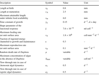
We denote the length of a Daphnia individual byx and bySthe concentration of algae. For meanings and values of parameters, we refer to Table1. In the absence of consump-tion, the dynamics of an algae populationSare described by a ratef (S)=a1(Smax−S) for chemostat models orf (S)=a2S(1−SS
Table 1 Parameter specification as in de Roos et al. (1990)
Description Symbol Value Unit
Length at birth xb 0.8 mm
Length at maturation xA 2.5 mm
Maximum attainable length
under infinite food availability xm 6.0 mm
Time constant of growth γg 0.15 d−1, d=day
Shape parameter of the
functional response ξ 7.0×10⁻⁶ ml·cell−1
Maximum feeding rate
per unit surface area νS 1.8×10⁶ cell·mm−2·d−1 Fraction of ingested energy
channeled to growth and maintenance κ 0.3 –
Maximum reproduction rate
per unit surface area rm 0.1 mm−2·d−1
Random death rate of Daphnia μ variable d−1
Maximum concentration of algae
in the absence of Daphnia Smax variable cell·ml−1 Flow-through rate in case of
chemostat algal dynamics a1 0.5 d−1
Flow-through rate in case of
logistic algal dynamics a2 0.5 d−1
equilibria(b, S)=(0, Smax)and(b, S)=(0,0)and concentrate on interior equilibria. The equilibrium growth rate is given as
gx, S=γg
xmfr
S−x, (57)
where here and in the following we denote the (Holling type II) functional response as
fr
S:= ξ S
1+ξ S.
The equilibrium birth rate and consumption rate become
βx, S=
0, xb≤x≤xA,
rmfr(S)x2, xA≤x,
(58)
γx, S=νSfr
Sx2. (59)
Finally, we assume that the mortality rate is a constant, which we also denote byμ, i.e., thatμ(x, S)≡μ. In de Roos et al. (1990), it is motivated that from a biological point of view a good choice for the two free parameters is the background mortality for Daphnia
Table 2 Numerical integration with Algorithms3.2and3.3
S μ bε(S, μ) Gε(S, μ)
5.000000E+05 0.300000 5.156976E−03 −0.133576
in (25). Next, we recall that we locate the first curve point by fixingα1and then apply-ing a Newton algorithm to find the other components of the curve point. In this regard for the Daphnia models, a good choice is to setα1:=μfor the computations of existence boundaries andα1:=Smaxandα2:=μfor stability boundaries. As accuracy constants for numerical differentiation, we useδ1:=1.0E–4,δ2:=1.0E–7. Finally, in the computations where integration is stopped by decreased survival, we defineε:=10−9as the survival probability at which integration stops. If we stop integration whenareachesAmax, we set
Amax=70 years.
4.2. Existence boundaries
In the following, we show the results of the implementation of Algorithms3.2,3.3,3.7, and3.9.
4.2.1. Numerical integration for existence boundaries
We show a numerical example for the computation ofGε(S, μ)andbε(S, μ)for given
S, μwith Algorithms3.2and3.3in Table2. The isolated Algorithm3.2can be used to find out how close to the curve a guess is, and thus also to find an initial guess which leads to convergence. The numerical example shown is such a guess. We stop integration when
areachesAmax.
4.2.2. Tracing of existence boundaries
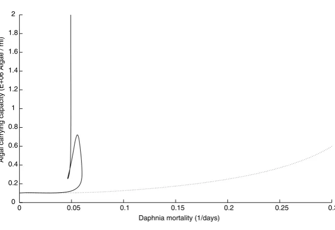
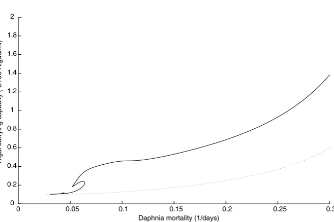
We have traced existence boundaries for Daphnia models with Algorithms 3.2, 3.7, and3.9. For Daphnia magna as parametrized in Table1, this is the dotted line in Figs.3–4 and6–9.
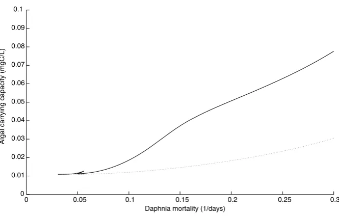
In Figs.11–13, we have plotted the data for the model of Daphnia pulex feeding on
Chlamydomonas rheinhardii in (de Roos,1997). The model has the same specification of vital rates in terms of parameters as the Daphnia magna model, but the parameters have different values. The values used are nowxb=0.6,xA=1.4,xm=3.5,Fh=1ξ =0.164,
γg=0.11,rm=1.0,νS:=0.007,anda2:=0.5. We use the same values for stopping the integration as for the Daphnia magna model.
4.3. Stability boundaries
To specify the ODE for the computation of stability boundaries, it remains to compute the partial derivatives of the vital rates in a point(X(a, S), S), as well as their one-sided limits inxAfor givenS. These partial derivatives are in the notation of Section2.3.3
g1(a)= −γg, g2(a)=γgxmfr
S, frS= ξ (1+ξ S)2,
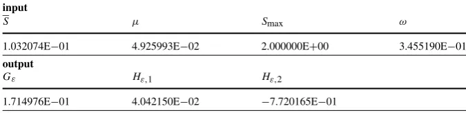
Table 3 Numerical integration with Algorithm3.10.Hε,1andHε,2denote the two components ofHε input
S μ Smax ω
1.032074E−01 4.925993E−02 2.000000E+00 3.455190E−01
output
Gε Hε,1 Hε,2
1.714976E−01 4.042150E−02 −7.720165E−01
β1(a)=
0, xb≤X(a, S) < xA,
2rmfr(S)X(a, S), xA≤X(a, S),
β2(a)=
0, xb≤X(a, S) < xA,
rmfr(S)X2(a, S), xA≤X(a, S),
γ1(a)=2νSfr
SXa, S, γ2(a)=νSfr
SX2a, S.
The one-sided limits are
g−=g+=γg
xmfr
S−xA
, μ−=μ+=μ,
β−=0, β+=rmfr
SxA2, γ−=γ+=νSfr
SxA2.
4.3.1. Numerical integration for stability boundaries
In Table3, we show an example of the computed values ofFε(S, μ, Smax, ω)for givenS,
μ,Smax, andωwith Algorithm3.10. Like in the one-parameter problem, we can use the isolated algorithm for numerical integration to find an initial guess that leads to conver-gence. We show such a guess in Table3, where we stopped integration ata=Amax.
4.3.2. Stability boundaries
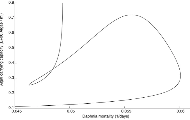
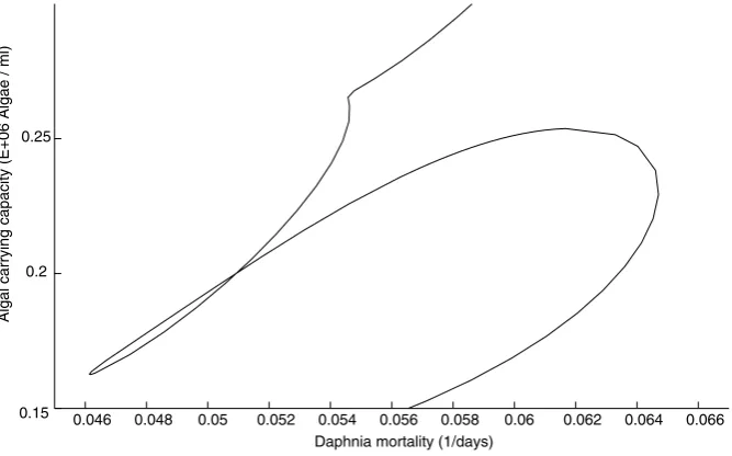
We then trace stability boundaries for Daphnia magna with Algorithm3.9, which calls Algorithm3.10for numerical integration, Algorithm3.7to locate the first point on the curve and for correction and Algorithm3.3for updates of the population birth rate. The resulting curves are shown in Figs.3–10. In Figs.4,7, and9, we have used the reaching ofAmaxas stopping mechanism to have the same conditions as in de Roos et al. (1990). The figures correspond with Fig. 2 in de Roos et al. (1990). In Figs.11and13, we have computed the stability boundaries for the Daphnia pulex model in de Roos (1997). Fig-ure13coincides with Fig. 7 in this reference. In Fig.5, resp.10and12, we depict the same graph as in Fig.4, resp.9and11, on larger scales to show details, such as windings of the curves.
In the existence region near to the existence boundary, the number of roots in the right-half plane is zero. We call the computed curve suggestively a stability boundary, since we