Matrix Estimation with STAQ

(1)

July 14, 2018

MASTER THESIS

MATRIX ESTIMATION

WITH STAQ

Bernike Rijksen

Applied Mathematics

Discrete Mathematics and Mathematical Programming Supervisors:

(2)

Preface

This master thesis finishes my master Applied Mathematics at the University of Twente. In September I started my internship at DAT.Mobility, which is part of the Goudappel Groep. Goudappel Groep gives advises on all kinds of mobility problems and within DAT.Mobility all expertise on the area of big data, model methodology, geographic information systems and software development is brought together. My assignment was to study the matrix estimation problem for the assignment model STAQ. And although this problem is only a small subproblem within a big system of models which work together to forecast traffic flows on a network, I like the idea that this research attributes to practice.

An important part of my internship was to develop an understanding for the given problem and the related models. Herein I have learned a lot from my supervisors at DAT.Mobility, Luuk Brederode and Luc Wismans. They provided me with the right literature and models and were always willing to answer my questions. By reading papers and testing different hypotheses on small test networks in Excel and Matlab, I obtained knowledge and feeling for the given problem, which resulted in many ideas and conclusions. But there was a lot more to investigate. Therefore I decided to continue with this subject as my final master project. I am happy with this decision because during the past months I have been able to analyse and answer many of the open questions there were at the end of my internship. The weekly discussions with Georg Still have attributed a lot to these results. He was always helpful and critical on my work. Although the matrix estimation method for STAQ is still in development, I am proud of what I reached. Luuk Brederode will continue working on the developed matrix estimation method and I hope he will keep me informed.

(3)

Abstract

This research focuses on the matrix estimation problem for the assignment model STAQ. In the matrix estimation process, additional road information is used to refine the OD-matrices which are estimated in the first three steps of the four step model. The chosen assignment model, in this case STAQ, is needed in this matrix estimation process. As such, the matrix estimation problem is typically expressed as a level optimization problem. Because bi-level problems are known to be NP-hard, in practice heuristic methods are used to search for solutions. Conventional matrix estimation methods as developed for traditional static traffic assignment models are not directly suitable for STAQ. The approximations of the link flows as considered in these heuristic methods cannot cope with capacity constraints. Therefore Brederode et al. [5] propose a matrix estimation method for STAQ, in which the link flows are approximated using a first order Taylor approximation. In this study it has been shown that the current approach to determine the sensitivities of the assignment matrix to changes in the OD-demands, which are required in the first order Taylor approximation of the link flows, can lead to significant errors. It should be investigated on large scale networks how big those errors are. It might be needed to adapt the way of approximating the link flows or to choose a different heuristic approach. Furthermore from the characteristics of the simplified upper level optimization problem as considered within the proposed matrix estimation method it has been concluded that this optimization problem can be solved best using the quadprogsolver in Matlab. However also the currently implemented

(4)

Notation List

N set of nodes

R ⊆N set of origins

S ⊆N set of destinations

RS |R×S| set of OD-pairs

P set of paths

˜

P ⊆P set of paths with travel time measurements

A set of directed links

˜

A ⊆A set of directed links with count measurements

I ⊆A set of inlinks

J ⊆A set of outlinks

IJ set of turns

D vector of OD-demands

Q |P| vector of path demands

T |IJ| vector of turn demands

Y |A| vector of link demands

y |A| vector of link flows ˜

y |A˜| vector of observed link flows

t |IJ| vector of turn flows

τ |P| vector of path queueing delays ˜

τ |P˜| vector of observed path queueing delays

α |IJ| vector of turn based reduction factors D |R×S| OD-matrix

A |A˜| × |R×S| assignment matrix B |A˜| × |P| crossing fraction matrix P |P| × |R×S| route fraction matrix

Drs ∈D demand from originrto destination s

Qp ∈Q demand on pathp

Tij ∈T turn demand from inlinkito outlinkj

Ya ∈Y demand on linka

ya ∈y flow on linka

˜

ya ∈y˜ observed flow on linka

tij ∈t flow from inlinkito outlink j

τp ∈τ average path queueing delay

˜

τp ∈τ˜ observed average path queueing delay

αij ∈α reduction factor on turnij

Ars

a ∈A fraction of demand from OD-pairrsthat flows over linka

ˆ

αp

a ∈B reduction factor on pathptill linka

ψrs

(5)

Chapter 1 Background information

Mobility plays an important role in modern life. To improve and schedule traffic and transportation, models are used to forecast traffic flows on networks. The goal of this master thesis is to mathematically describe and solve a subproblem within a certain traffic model. More specific: I studied the matrix estimation problem for the four step traffic model with assignment model STAQ. This chapter provides the required background information about the four step model, the matrix estimation problem and the assignment model STAQ. In the next chapter the exact research question of this master thesis is introduced.

1.1 Four step model

The four step model is the most commonly used traffic and transportation model to forecast traffic flows on networks. In this model the network of the studied area is represented in the form of a directed graph (N, A), whereN are the nodes which represent the junctions in the network andAare the links which represent the roads in the network. The studied area is divided in several zones for which characteristic socio-economic data is available. All these zones are connected to the network via centroids, which are one or more nodes in the centre of the zone. Trips in the network always start and end at these centroids. Commencing with this directed graph and the available socio-economic data, the four step model estimates trips per transport mode and the use of the network in terms of flows per link. The model consists of the following steps [9] [13]:

1. Trip generation In the first step, based on the available socio-economic data, the number of people arriving in and departing from each zone are determined. After this step it is clear how many trips originate and terminate at each centroid, but the origin and destination of specific trips are not yet connected.

2. Trip distribution In the second step the number of trips between each origin and destination pair (OD-pair) is determined. This number is called the trip demand of the OD-pair. The gravity model1is a frequently used method to obtain these trip demands. The trip demands of all OD-pairs

(8)

are represented in a matrix, this matrix is called the origin-destination matrix (OD-matrix). So the OD-matrix describes the number of trips from every centroid in the studied network to every other centroid in the network.

3. Modal split In the third step for each OD-pair it is decided how the trips are divided over different transport modes. Examples of transport modes are car, public transport and bicycle. After this step the number of trips between all OD-pairs are known per mode (there is determined an OD-matrix per mode), but it is not known which route on the network each trip will take. In practice step 2 and step 3 are often combined.

4. Assignment Finally in the fourth step the trip demands of all OD-pairs are distributed along the network. So for each trip it is determined which route in the network it will take. There is a wide variety of models developed to deal with this assignment problem, these models are called assignment models. When all traffic demand is assigned to the network, values for the flows and speeds on the links can be deduced.

So following these four steps, the four step model finds a forecast of the traffic flows on a network. In practice a feedback loop is performed within the four step model. This is needed because the gravity model used in step two requires the travel time between each OD-pair as an important aspect of the generalized costs2_{between OD-pairs, but there are no travel times other then free-flow travel} times known before the fourth step.

1.2 Assignment models

As described, there is a wide variety of assignment models available. Within this study the assignment model STAQ is used (studied), which stands for Static Traffic Assignment with Queueing. The assignment model STAQ is explained in section 1.4. In this section first a general introduction to assignment models is given, such that the matrix estimation problem and the assignment model STAQ can be explained and placed within this context.

Traffic assignment models describe the interaction between road travel demand and road infrastructure supply. Given the travel demand on a network, assign-ment models describe how this travel demand is distributed along the network. All assignment models consist (implicitly or explicitly) of a route choice submodel and a network loading submodel. The route choice submodel determines path flows, based on travel demands and travel times. The network loading submodel propagates path flows through the network and yields travel times. This is shown in figure 1.1. Bliemer et al. have introduced a theoretical framework for the classification of traffic assignment models. Their classification is shortly discussed in this section, because it gives insight in the different assignment models available. In this theoretical framework assignment models are classified on their spatial, temporal and behavioural assumptions. In the remainder of this section the different model types within these three model classes are briefly

2_{For simplicity in the rest of this report the generalized costs are considered to consist of}

(9)

[image:9.595.210.382.125.249.2]

Figure 1.1: Interaction between travel demand and infrastructure supply [2].

explained. For more details the reader is referred to their article “Genetics of traffic assignment for strategic transport planning” [2].

1.2.1 Route choice submodel

Within the theoretical framework the behavioural assumptions describe the route choice submodel. The route choice submodel determines path flows based on given travel demands and considered travel times. To describe the route choice submodel, the behavioural assumptions define how the considered travel times are determined, and how the travellers are assumed to choose their routes. As a result of the behavioural assumptions, the theoretical framework distinguishes between three model types:

1. Equilibrium models In an equilibrium model an equilibrium flow is sought for in which no traveller can unilaterally change routes to improve his or her travel time. Congested travel times are considered by iterating between the route choice submodel and the network loading model. The routes can be chosen in a deterministic or stochastic way.

2. One-shot models In an one-shot model a single network loading is performed to determine the travel times on the routes. The routes are usually chosen using a logit-model (stochastic route choice).

3. All-or-nothing models In an all-or-nothing model typically free-flow travel times are used. The routes are chosen such that all travellers follow the fastest route (deterministic route choice). An all-or-nothing model is a special case of a one-shot model.

(10)

In an equilibrium model congested travel times are considered. The difficulty of considering congested travel times is that these travel times are not fixed. The level of congestion and hence the travel time on a route is depending on the route choice, and the route choice is on its turn depending on the amount of congestion on each possible route. Because of this interaction between route choice and travel times, equilibrium models iterate between the route choice submodel and the network loading submodel to account for congested travel times. The route choice submodel calculates path flows which are used by the network loading model to update the travel times. Then these updated travel times are used by the route choice submodel to calculate new path flows (etc.). Note that in one-shot models and all-or-nothing models the travel times are considered to be fixed. Hence these models do not iterate between the route choice submodel and the network loading submodel, and thereby these models do not consider congested travel times.

The route choice in an equilibrium model can be determined in a stochastic way, like in an one-shot model, or in an deterministic way, like in an all-or-nothing model. Hence one-shot models and all-or-nothing models can be seen as a single iteration of an equilibrium model. In an equilibrium model the route choice tends to comply with Wardrop’s first principle:

“The journey times in all routes actually used are equal and less than those which would be experienced by a single vehicle on any unused route” [19].

So an equilibrium is sought for, in which no traveller can unilaterally change routes to improve his or her travel time. Such an equilibrium is called a User Equilibrium (UE). A feedback loop is performed between the route choice submodel and the network loading model till this equilibrium state is reached. The travellers are assumed to be non-cooperative, so they exhibit selfish behaviour. This is in contrast to system optimal models, which minimize the total (or average) travel time in the system and assume travellers to cooperate.

1.2.2 Network loading submodel

Within the theoretical framework the spatial assumptions describe the network loading submodel. The network loading submodel loads the path flows on the network and yields travel times. The spatial assumptions define if and how the network loading submodel accounts for congestion (delays and queues). As a result of the spatial assumptions there are four model types distinguished. They are described below in a decreasing order of capability. The less capable model types can be derived from the more capable model types by making simplifying assumptions:

(11)

2. Capacity-constrained models In capacity-constrained models, there are no constraints on the storage of queues on road segments and as such spillback does not occur. These models are suitable for light to heavy traffic conditions in which short queues can form.

3. Capacity-restrained models In capacity-restrained models, flows can also exceed the physical road capacity and, therefore, queues are not described explicitly. These models are only suitable for light to medium traffic conditions in which the flow does not exceed the capacity, but some slight delays may occur due to increasing density.

4. Unrestrained models In unrestrained models, there are fixed (usually free-flow) travel conditions and travel times. These models are only suitable for light traffic conditions in which flow increases linearly with density, indicating that vehicles drive at maximum speed.

[image:11.595.166.421.535.640.2]

Actually the more capable the model type, the better these models reflect the theoretical relationship which exists between flow and density. This theoretical relationship between the flow and density can be empirically observed from traffic counts and can be described in a fundamental diagram (see figure 1.2). Each point in this fundamental diagram represents a specific steady traffic state. When the density is below the critical density, there is no congestion and no queues appear. The corresponding branch of the fundamental diagram is called the free-flow branch. Densities higher then the critical density are a result of congestion and queues on the road. This branch in the fundamental diagram is called the congested branch. All model types explicitly or implicitly3 _{assume a} fundamental diagram. In figure 1.3 for each model type an example of a funda-mental diagram is shown. The fundafunda-mental diagram of the least capable model type only reflects part A of the theoretical fundamental diagram in figure 1.2 correctly. The more capable the model type, the better it reflects the theoretical fundamental diagram. The most capable model type is suitable for all given traffic conditions and hence reflects all parts of the theoretical fundamental diagram correctly (A, B, C and D).

Figure 1.2: Theoretical relationship between flow and density [2].

3_{For the unrestrained and capacity-restrained model types, in practice only a travel time}

(12)

[image:12.595.170.422.129.191.2]

Figure 1.3: Fundamental diagrams [2].

While the fundamental diagram only shows flows (veh/h) and densities (veh/km), the speed of a vehicle (km/h) can be determined using the fundamental relation-ship that speed equals flow divided by density [2], or equivalently:

flow = speed·density (1.1)

So, given the flow and density, it is possible to determine the corresponding speed and hence the corresponding travel time4 _{on a link. Note that for unrestrained} and capacity-restrained model types, given a link flow, the corresponding density can be uniquely determined from the fundamental diagram. The travel times are separable; They are only depending on the flow on the link itself. Whereas for capacity- (and storage)-constrained model types, given a link flow, also the corresponding density is needed to determine the speed and hence the travel time on the link from the fundamental diagram5_{. The travel times are non-separable;} The travel time on a link depends on the level of congestion on the link, which on its turn depends on the flows on all other links.

1.2.3 Temporal assumptions

Finally within the theoretical framework the temporal assumptions define if and how a time dimension is considered within the assignment model. As a result of the temporal assumptions the theoretical framework distinguishes between three model types. They are described below in decreasing order of capability:

1. Dynamic models Dynamic models consider a time-varying travel demand and generally (but not necessarily) multiple time periods for route choice. Within each time period there exist smaller time steps for network loading. In these models variations over time in path flows, link flows and travel times are explicitly taken into account.

2. Semi-dynamic models Semi-dynamic models often consider only a single step for network loading within each route choice period, but traffic flows can be propagated between route choice periods. These models can be seen as a sequence of static models, in which the result from a previous period is taken into account in the next period.

3. Static models Static models consider a stationary travel demand and only a single time period for the route choice and the network loading. It is assumed that traffic outside this time period does not influence flows or

4_{The travel time on a link (h) equals the length of the link (km) divided by the speed}

(km/h) on the link.

(13)

[image:13.595.169.427.123.211.2]

Figure 1.4: Relation time periods and travel demand [2].

travel times in the considered period. Within the network loading step all traffic reaches the destination. Static models result in an average image of the traffic in the considered time interval.

In figure 1.4 it is shown how static, semi-dynamic and dynamic models represent the travel demand. The more capable the model, the better it reflects the time-varying travel demand (the red line). Note that this figure only visualizes the differences between the model types in travel demand, other relevant differences have been described above.

1.2.4 Classification

In the previous subsections the different model types within the three model classes of the theoretical framework for the classification of traffic assignment models are described. The behavioural and temporal assumptions distinguish between three model types and the spatial assumptions distinguish between four model types. Combining the three different model classes, 36 different assignment model types can be described. This is shown in the framework in figure 1.5. Note that not all model types distinguished in the framework exist or can exist in practice. The goal of this framework is to make it possible to classify and compare existing traffic assignment models.

The least capable model type according to this framework is a static unrestrained all-or-nothing traffic assignment model. The most capable model type is a dynamic capacity and storage-constrained equilibrium traffic assignment model. Of course it seems best to build and always use the most capable model. But it turns out that this model is not ideal in practice. The dynamic capacity and storage-constrained equilibrium traffic assignment model is poorly scalable, data intensive and it has even been proven that there does not always exist an equilibrium for this model type [6]. Therefore, to support policy development and planning in strategic applications on large scale congested networks, the assignment model STAQ is developed [4]. STAQ circumvents problems with scalability and data-intensiveness, because this model does not consider a time dimension. The assignment model STAQ is a static capacity-constrained and6 capacity- and storage-constrained assignment model which can be applied as an equilibrium model, and will be further introduced in section 1.4. First, in the next section the matrix estimation problem introduced.

(14)

[image:14.595.186.396.132.247.2]

Figure 1.5: Framework classification traffic assignment models, edited from [2].

1.3 Matrix estimation problem

The matrix estimation problem for the assignment model STAQ is the central subject of this master thesis. This section provides a general introduction to the matrix estimation problem.

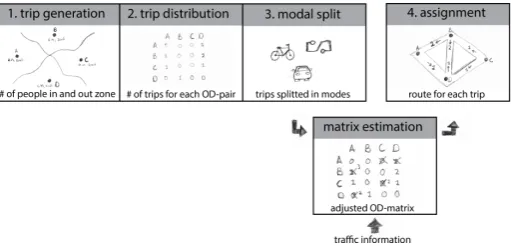
Matrix estimation is a process which aims to improve the results of the four step traffic model by adding exogenous information. In the four step traffic model, after step three, OD-matrices have been determined per mode. These OD-matrices are determined by the behavioural models in the first three steps of the four step model (see section 1.1). The behavioural models do not always guarantee good results, because the socio-economic data (survey-data) used, only describes the average mobility behaviour over an entire study area. To refine the results of the four step traffic model, additional traffic measurements can be used to improve the modelled OD-matrices. This process is called matrix estimation. In figure 1.6 the position of the matrix estimation process within the four step traffic model is visualized. The traffic measurements which are used for this process can be of many types and sources, most frequently used are traffic counts. Traffic counts register the traffic flow on a certain location in the network.

To improve a modelled OD-matrix using traffic counts, the modelled OD-matrix should be adjusted such that it better fits to measured traffic flows. The difficulty is that the adjusted OD-matrix cannot be directly compared with the measured traffic flows. matrices describe the traffic demand for each OD-pair and the traffic flows caused by these OD-demands are only known after an assignment is performed. In other words, there is no one-to-one correspondence between OD-matrices and traffic counts. Therefore the assignment problem, in which the demand of a given OD-matrix is distributed along the network, is embedded within the matrix estimation problem7[13]. Because of this embedded assignment problem, the matrix estimation problem is typically expressed as a bi-level optimization problem. In the upper level the modelled OD-matrix is improved based on available traffic measurements, while in the lower level the

7_{So note that the chosen assignment model within the four step traffic model is not only}

(15)

[image:15.595.168.424.126.249.2]

Figure 1.6: Matrix estimation within the four step model.

traffic assignment problem is solved. When traffic counts are the only traffic measurements used, the matrix estimation problem is formulated as follows:

min

D F(D) =αf1(D, D

0_{) + (1}

−α)f2(y,y˜)

s.t. y= Assign(D)

D≥0

(1.2)

D vector/matrix of estimated OD-demands

D0 _{vector/matrix of prior (modelled) OD-demands}

y vector of estimated link flows ˜

y vector of observed link flows

f1 distance function

f2 distance function

α ∈[0,1] weighting factor

Note that in the upper level of this bi-level optimization problem not only the distances between the observed and estimated link flows, but also the distances between the modelled (prior) and estimated OD-demands are minimized. This term is included, to not deviate too much from the OD-matrix as estimated in the first three steps. The distance functionsf1andf2should be defined to make the problem concrete. These distance functions can be of many forms, for an overview the reader is referred to the master thesis of Smits [13]. Furthermore the weighting factorαgives the decision maker the opportunity to express his or her confidence in the prior matrix against the traffic counts. A smaller value ofα

(16)

[image:16.595.201.392.126.243.2]

Figure 1.7: The assignment matrix.

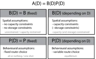
In the lower level of the bi-level optimization problem, an assignment model Assign(D) is embedded, which can be any of the available assignment models. The assignment model distributes a given demandDalong the network, which results in flows y(D) on all links. According to Frederix et al. [8], for each possible assignment model the relation between the given OD-demands and the resulting link flows can be described by an assignment matrix A(D). This assignment matrix can be further subdivided into a crossing fraction matrix and a route fraction matrix:

y(D) =A(D)D,

=B(D)P(D)D. (1.3)

D vector of OD-demands,|R×S|

y(D) vector of estimated link flows,|A˜| A(D) assignment matrix,|A˜| × |R×S| B(D) crossing fraction matrix,|A˜| × |P| P(D) route fraction matrix,|P| × |R×S|

˜

A set of links with count measurements

R set of origins

S set of destinations

P set of paths

The elements of the crossing fraction matrixB(D) express the proportion of a route flow that passes a link, thereby these elements describe the spatial propa-gation of the route flows through the network by the network loading submodel8. The elements of the route fraction matrixP(D) express the proportion of an OD-flow choosing a certain route, thereby these elements reflect the behavioural assumptions of route choice submodel. Finally the temporal assumptions of the assignment model are reflected in the dimensions of the assignment, crossing fraction and route fraction matrices. If more time periods are considered, these dimensions are correspondingly enlarged. It can be concluded that the assign-ment matrixA(D) is depending on the chosen assignment model.

8_{When there are no capacity and storage constraints considered, the crossing fraction matrix}

(17)

In figure 1.7 it is shown that for some assignment models the crossing fraction matrix and the route fraction matrix are fixed matrices; They are not depending onD. It is interesting to note that if both the route fraction and the crossing fraction matrix are assumed to be fixed matrices, then the matrix estimation problem can be reformulated to a single level problem. In this case the assign-ment matrix is the same (and hence explicitly known) for all givenD, so there exists a linear relationship between the link flows and the OD-flows and as such the vector of estimated link flowsy can be formulated explicitly as a function of the OD-demandD. Hence the given bi-level matrix estimation problem can be reformulated as a single level problem. Such a reformulation to a single level problem is possible for all assignment models for which the assignment matrix A(D) is known explicitly. The assignment matrix of the assignment model STAQ cannot be expressed explicitly as a function of the OD demands. Therefore the matrix estimation problem for STAQ is (remains) a bi-level optimization problem.

1.4 STAQ

In this section the traffic assignment model STAQ is introduced. STAQ stands for Static Traffic Assignment with Queueing. As the name already indicates, STAQ can be seen as a static traffic assignment model. So the results of STAQ give an average image of the traffic in the considered time interval. In the next two subsections the route choice submodel and the network loading submodel of the assignment model STAQ are described, following the paper of Brederode et al [4]. Subsequently STAQ is placed within the theoretical framework for the classification of traffic assignment models as described in subsection 1.2 and its capability is discussed.

1.4.1 Route choice submodel

In figure 1.8 the modelling framework for the assignment model STAQ is shown. When used as an equilibrium model, STAQ iterates between its route choice submodel and its network loading submodel, such that congested travel times are considered. The main characteristics of STAQ are derived from its network loading model and as such its route choice submodel is interchangeable [4]. The route choice submodel within STAQ as considered in this study, consists of three components which interact to determine path flows from the given travel times:

• Route set generator The route set generator creates a set of routes based upon a given transport network.

• Route choice model The route choice model uses generalized costs, which are mainly based on the travel times calculated by the network loading model, to compute route fractions for all route alternatives between an OD-pair.

(18)

[image:18.595.168.423.125.251.2]

Figure 1.8: STAQ modelling framework, edited from [4].

1.4.2 Network loading submodel

The network loading submodel within STAQ consists of four different components which interact to propagate the given route demands through the network and calculate the resulting travel times:

• Link model The link model describes for each link the relation between flow and density in the form of a fundamental diagram. It determines from the path demands as given from the route model in interaction with the node model the corresponding link flows.

• Node model The node model seeks for a consistent solution in terms of flows transferred over an intersection. It accounts for flow restrictions due to merge and diverge interactions between flows. This model can transfer the effect of capacity restrictions on downstream to upstream links and the effect of demand changes on upstream to downstream links.

• Junction model The junction model accounts for the effect of limited supply due to conflict points on a junction itself and the way the junction is regulated. Furthermore it calculates travel time delays due to passing a junction.

• Travel time calculator The travel time calculator derives travel times from the output as calculated by the link model, node model and junction model.

STAQ can be applied to congested networks in which queues can grow longer than the road length and spillback to upstream road segments occurs. To deal with congestion the network loading model considers two phases: a squeezing phase and a queueing phase. The squeezing phase deals with the flow metering effect of congestion, assuming capacity but no storage constraints and the queue-ing phase deals with the spillback effect of congestion, assumqueue-ing both capacity and storage constraints. STAQ-squeezing can also be used as a stand-alone network loading model, but STAQ-queueing needs the squeezing phase outcomes for initialisation9_.

9_{The queueing phase uses initial sending and receiving flows for every link as calculated by}

(19)

[image:19.595.199.388.124.192.2]

Figure 1.9: Fundamental diagrams STAQ -squeezing (left) and -queueing (right) [4].

Both phases of STAQ use the same node model and the same junction model, but different link models. The link models differ by the form of their funda-mental diagram. This is shown in figure 1.9. The free-flow branch (blue) of both fundamental diagrams is identical. The fundamental diagrams differ in the congested branch (red). The congested branch of the fundamental diagram for STAQ-squeezing satisfies a maximum flow constraint. In this way the squeezing phase takes into account flow metering: the flow on a link can never become higher than the maximum flow of capacity of that link. However the maximum density is not constrained. As a consequence in the squeezing phase vertical queues are implied. All demand on a link that exceeds the maximum capacity forms a vertical point queue on the upstream node of this link10. Hence the squeezing phase detects the locations and the severity of active bottlenecks in the network. Then the spillback effect of congestion is considered in the next phase, the queueing phase. The fundamental diagram of STAQ-queueing constrains both the flow and the density. Therefore the queueing phase accounts for both the flow metering and the spillback effects. The fundamental diagrams in figure 1.9 are meant to show the difference between the squeezing and queueing phase, they are not explicitly implemented in the models.

In practice the network loading model first considers the squeezing phase and then the queueing phase. During the squeezing phase the STAQ algorithm iterates11 between the network loading submodel (squeezing) and the route choice submodel till an User Equilibrium is approximated. After this phase the bottlenecks in the network are determined. Then, to determine the spillback and secondary effects of these bottlenecks, in the queueing phase the STAQ algorithm performs one iteration with the network loading submodel (queueing). Only one iteration is performed, because in real world applications on heavily congested networks it is not always possible to approximate an equilibrium to a level that is sufficient for strategic transport model applications [6]. Although no time dimension exists with respect to the in- and output of STAQ, the queueing phase uses internally a time dimension to allow for the spatial interaction between all different spillback and flow metering effects. Brederode et al. [4] describe that the main reason to split the algorithm in two phases is to maintain scalability when calculating spillback and secondary effects of bottlenecks. Additional reasons are that the flow metering and spillback effects can be analysed separately and that the squeezing phase compensates for the lack of a pre-study-period warm-up.

10_{Such an assignment model is called a residual queueing model.}

11_{Note that this only holds when STAQ is used as an equilibrium assignment model, otherwise}

(20)

[image:20.595.184.397.134.246.2]

Figure 1.10: Placement of STAQ within the framework, edited from [2].

1.4.3 Capability of STAQ

It can be concluded that STAQ is a static traffic assignment model and from the fundamental diagrams in figure 1.9 it can be seen that STAQ is capacity-constrained in the squeezing phase and capacity- and storage-capacity-constrained in the queueing phase. Note that STAQ technically spoken is not static in the queueing phase, but its input and output are both static of nature. The theoretical framework in figure 1.10 shows that STAQ is a more capable assignment model than the traditional static traffic equilibrium assignment (STA) models, which assume separable monotonously increasing travel time functions and hence are unrestrained or capacity-restrained models. Traditional STA models cannot cope with capacity constraints, nor represent flow metering and queue formation, while STAQ takes into account these physical effects of congestion. Therefore, according to Brederode et al, STAQ is a viable alternative for traditional STA models to support policy development and planning in strategic applications on large scale congested networks [5]. STAQ combines the advantages of classical static and typical12 _{dynamic assignment models; It is a computationally fast} and scalable model which takes into account the physical effects of congestion. Note that in figure 1.10 the traditional STA model, STAQ and the typical DTA model are indicated as equilibrium assignment models. While comparing these three model types they are considered to be equilibrium models. However, they can also be used as a one-shot or AON assignment models. The algorithms as used within STAQ are explained in detail in chapter 3.

12_{Nowadays dynamic models are typically capacity- (and storage-) constrained model types.}

(21)

Chapter 2 Introduction

In the previous chapter the matrix estimation problem and the assignment model STAQ have been introduced. Recall that the assignment problem, and hence the chosen assignment model, is embedded within the matrix estimation problem. This research contributes to the development of a solution method for the matrix estimation problem with the assignment model STAQ. Within this chapter the goal of this research and the research question for this master thesis are introduced and motivated. Besides, the corresponding solution approach and the structure of this report are explained.

2.1 Research motivation

Matrix estimation methods for traditional static traffic assignment (STA) models are studied extensively and are readily available [5]. Generally these assignment models assume separable monotonously increasing travel time functions (see subsection 1.2.2), and as such, using these models it is relatively easy to determine how the prior OD-matrix should be adjusted to achieve similar modelled and observed link flows. Contrary to traditional STA models, STAQ takes into account capacity constraints and represents flow metering and queueing effects. This results in a more realistic, but also more complex assignment model. The implicitly considered travel time functions within STAQ are not separable any more; The travel times on the links are not only depending on the flow on the link itself, but also on the flows on all other links. This makes it more complex to determine how the prior OD-matrix should be adjusted to achieve similar modelled and observed link flows. Therefore, available matrix estimation methods, which are developed for traditional STA models, are not directly suitable for the assignment model STAQ. This research aims at developing a suitable matrix estimation method for STAQ. Within this master thesis a specific method for matrix estimation with STAQ is investigated. This proposed method is developed by Brederode et al. [5]1 _{(it is still under development) and is based} on the conventional matrix estimation method for traditional STA models. The conventional matrix estimation method for traditional STA models and the proposed matrix estimation method for STAQ are discussed in the next two subsections.

(22)

2.1.1 Conventional matrix estimation method

Generally the matrix estimation problem is a bi-level optimization problem (see section 1.3); In the upper level problem the distances between the prior and estimated OD-matrix and between the observed and estimated link flows are minimized. However, the estimated link flows corresponding to the estimated OD-matrix, are (for most assignment models) only known explicitly after solving the assignment problem for this OD-matrix, hence after solving the lower level assignment problem. So the evaluation of the upper level objective function requires solving the lower level optimization problem, whose functional form is generally unknown. It is important to realize that bi-level problems are in-trinsically hard to solve. They are neither differentiable anywhere nor convex. This holds even when the objective functions of the upper level and lower level and the constraints are all linear, because the objective function of the upper level is decided by the solution function of the lower level problem and therefore is neither linear nor differentiable [18]. Bi-level problems are even shown to be NP-hard [1], which implies that they cannot be solved to optimality within polynomial time. Therefore in practice, heuristic methods are used to search for solutions which are not guaranteed to be optimal or perfect, but which are sufficient for practical applications.

To solve the bi-level matrix estimation problem for traditional STA models, conventionally a heuristic algorithm is used that iteratively assigns the OD-vector from the upper level into the lower level and then solves the upper level problem using the assignment matrix from the lower level to approximate the relationship between the OD-flows and the link flows [8]. In figure 2.1 this solution approach is shown. Recall from equation (1.3) in section 1.3 that the relationship between the OD-flows and the link flows is determined by the assignment model and is given by the assignment matrixA(D). Within the conventional solution approach for traditional STA models, the relationship between the OD-flows and the link flows in the upper level is approximated, using the assignment matrix from the previous lower level (STA model) assignment:

y(D)≈A(Dk−1)D,

=BP(Dk−1)D. (2.1)

y vector of estimated link flows

A(Dk−1₎ _{assignment matrix from previous lower level assignment}

D vector of OD-demands B crossing fraction matrix

P(Dk−1₎ _{route fraction matrix from previous lower level assignment}

The assignment matrix of a traditional STA model consists of a fixed crossing fraction matrix and a route fraction matrix which is depending on the OD-matrix. Traditional STA models do not take into account capacity and storage constraints and as such their crossing fraction matrix is equal to the (fixed) link path incidence matrix. However variations in route choice are taken into account, such that their route fraction matrix is depending on the OD-matrix2. So note

(23)

Dk_{= arg min}

D [w1f1(D, D0) +w2f2(y(D),y˜)]

wherey(D)≈A(Dk−1)D

s.t. D≥0

STA(Dk₎

Dk

[image:23.595.121.473.127.233.2]

k=k+ 1 A(Dk₎

Figure 2.1: Conventional solution approach for traditional STA model.

that a linear relationship between the link flows and the OD-flows is assumed in the upper level, whereas in reality this relationship is non-linear, because actually the route fraction matrix of a traditional STA model is depending on the OD-matrixD. But by performing iterations between the upper level problem and the lower level problem, the heuristic algorithm finds solutions which are sufficient enough for practice.

2.1.2 Proposed matrix estimation method

The conventional matrix estimation method for traditional STA models as introduced in the previous subsection, is not directly suitable for the assignment model STAQ. Contrary to traditional STA models, STAQ considers capacity and storage constraints, hence it takes into account the physical effects of congestion. As such, its crossing fraction matrix is not fixed, but is depending on the OD-matrix. If the conventional matrix estimation method for traditional STA models would be directly used for STAQ, the same linear relationship would be assumed:

y(D)≈A(Dk−1)D,

=B(Dk−1)P(Dk−1)D. (2.2)

y(D) vector of estimated link flows

A(Dk−1₎ _{assignment matrix from previous lower level assignment}

D vector of OD-demands

B(Dk−1₎ _{crossing fraction matrix from previous lower level assignment} P(Dk−1₎ _{route fraction matrix from previous lower level assignment}

However, in reality there are two sources of non-linearity for STAQ. Considering STAQ, not only the route fraction matrix, but also the crossing fraction matrix is depending on the OD-flows. So the assignment matrix is even more depending on the corresponding OD-matrix. Therefore, the approximation of the link flows as given in equations (2.2), turns out to be not suitable for STAQ3_{; Considering} STAQ, performing iterations between the upper level and lower level using (2.2), does not always lead to satisfying solutions.

(24)

This is why Brederode et al. [5] propose to approximate the relationship between the OD-demands and the link flows for STAQ in a different way; They propose a first order Taylor approximation4 around the previous OD-vectorDk−1:

y(Dk−1) =A(Dk−1)Dk−1,

y(D)≈A(Dk−1)Dk−1+δ A(D)D

δD

_D₌_Dk−1(D−D

k−1₎_. (2.3)

The main difference between the conventional approximation5of the link flows and the Taylor approximation as given in (2.3) is the second term in equation (2.3) [8]. This term incorporates the sensitivity of the assignment matrix to changes in the OD-demands; Hence using this approximation, the (first order) response of the lower level problem is taken into account in the upper level problem. This idea is adopted from Frederix et al. [8]. Frederix et al. describe that (even for traditional STA models) using the approximation as in (2.3) is theoretically more sound. Herein they refer to Yang [22] and Tavana [17], which both discuss the importance of including the response of the lower level problem when solving the upper level problem.

According to Yang [22] the conventional matrix estimation method for traditional STA models solves the matrix estimation problem as if it were a Cournot Nash game, while in reality it is a Stackelberg game. In a Cournot Nash game, the upper level and lower level problem are treated in a parallel (symmetric) way. Indeed this symmetry can be recognized in the conventional solution approach for traditional STA models. Both in the upper level and in the lower level optimization problem only the latest solution of the other sub problem is known. In an iterative way there is sought for a mutually consistent solution. However actually the matrix estimation problem is a bi-level optimization problem, and as such in reality it has an asymmetric hierarchical structure. In the upper level optimization problem not only the latest solution of the lower level, but also the reaction of the lower level to a given upper level decision is known. Such an asymmetric game is also known as a Stackelberg game [10]. So the matrix estimation problem is a bi-level problem and hence a Stackelberg game, and therefore the response of the lower level should be taken into account in the upper level optimization problem.

Although Frederix et al. [8] describe that it is theoretically more sound to use a first order Taylor approximation to approximate the link flows, they also describe why this approximation is not preferred in practice; For most assignment models the relationship between the OD-demands and the link flows is not explicitly known (see section 1.3), so the sensitivity of the assignment matrix to changes in the OD-demands cannot be exactly determined. It is possible to numerically approximate this sensitivity using finite differences, but therefore it is needed to perform a lower level assignment for each OD-pair in the network. In most practi-cal situations this leads to computation times which are not feasible. Therefore in practice many researchers use the conventional approximation of the link flows [8].

(25)

Dk_{= arg min}

D [w1f1(D, D0) +w2f2(y(D),y˜)]

where y(D)≈A(Dk−1)Dk−1+δ A(D)D

δD

_D₌_Dk−1(D−D

k−1₎ s.t. D≥0

STAQ(Dk₎

Dk

k=k+ 1 A(Dk_), δA(Dk₎

[image:25.595.122.474.127.239.2]

δDk

Figure 2.2: Proposed solution approach for STAQ.

Brederode et al. [5] explain in their paper that the sensitivity of the assignment matrix for STAQ can be easily determined without performing|RS|times a lower level assignment, by using the node model within STAQ. As such they conclude that the approximation of the link flows as given in (2.3) can be used efficiently for STAQ. Hence for STAQ it is possible to take into account the response of the lower level in the upper level optimization problem, while computation times remain feasible. In figure 2.2 the solution approach for the matrix estimation problem with STAQ as proposed by Brederode et al. [5] is shown. The exact method they propose to determine the sensitivity of the assignment matrix to changes in the OD-demands is explained in chapter 4.

2.2 Research question

The proposed matrix estimation method for STAQ as given in figure 2.2 is still under development. Currently it is possible to find realistic solutions on small test networks, if within STAQ only the squeezing phase is considered, fixed route choice is assumed and no junction modelling is applied. This simplified variant of STAQ is shown in figure 2.3. Of course finally it should be possible to solve the matrix estimation problem with STAQ for both the squeezing and queueing phase, using STAQ as an equilibrium model and applying junction modelling. To reach this, the idea is to first add route choice, so use STAQ as an equilibrium model, and then add junction modelling to the currently developed model. Finally not only the squeezing but also the queueing phase should be considered in the future.

The developed matrix estimation model for STAQ squeezing with fixed route choice and no junction modelling is implemented inMatlab. In the current model thefminconinterior point algorithm is used to solve the upper level optimization problem. However, it is not known if this solver is (most) suitable for the given optimization problem. Therefore I was asked to find out whether fminconof some other solver should be used, to solve the given upper level minimization problem. The corresponding research question is:

(26)

[image:26.595.168.423.125.252.2]

Figure 2.3: STAQ with no junction modelling, edited from [4].

2.3 Solution approach

To answer the research question, the given (upper level) optimization problem and the proposed solution method are mathematically formulated and analysed. Based on the mathematical characteristics of both the problem and the solution method a motivated choice for a suitable solver can be made. Analysing the given problem and solution method also resulted in recommendations for the further development of the matrix estimation method for STAQ.

(27)

Chapter 3 Problem formulation

In section 1.3 the matrix estimation problem has been generally introduced and formulated. In this chapter the studied matrix estimation problem for STAQ-uesqueezing with fixed route choice and no junction modelling is described in detail. Assumptions within the formulation of this problem are adopted from the developed matrix estimation method for STAQ [5].

3.1 Upper level problem

The formulation of the matrix estimation problem as given in section 1.3, is the conventional form of the matrix estimation problem. As mentioned before, this formulation only accounts for count information, hence for observed link flows. However, nowadays ever more types of (big) data are available to modellers. As such, in the developed matrix estimation method for STAQ, it has been chosen to also take the average travel times along paths into account. Furthermore, the developed method assumes that there is information available to determine for each link whether the link is in a free-flow traffic regime or in a congested traffic regime. The matrix estimation problem considered in this study has the following form:

min

D F(D) = minD w1f1(D, D

0_{) +}_w

2f2(y,y˜) +w3f3(τ,τ˜)

s.t. y, τ= Assign(D)

D≥0

+links in right traffic regime

(3.1)

D vector of estimated OD-flows

D0 vector of prior OD-flows

y vector of estimated link flows ˜

y vector of observed link flows

τ vector of estimated path queueing delays ˜

τ vector of observed path queueing delays

fi i∈ {1,2,3}, distance functions

(28)

In the upper level of this bi-level optimization problem not only the distances between the modelled (prior) and estimated OD-demands and the observed and estimated link flows are minimized, but also the differences between the observed and estimated path queueing delays. The average travel time on a path consists of the free-flow travel time and the average queueing delay on that path. And because the free-flow travel time on a path is fixed, only the path queueing delays are considered in the objective function. Note that the average travel time information is included in the objective function, while the traffic regime information is included in the constraints. Section 3.3 explains why the traffic regime information is needed to constrain the problem and formulates the traffic regime constraints explicitly.

The distance function used in the developed matrix estimation method is the squaredL2-norm. According to Smits [13], the advantage of this norm is that it does not rely on statistical assumptions. The distance functions in (3.1) get the following form:

f1(D, D0) = X

rs∈RS

(Drs−D0rs)

2

,

f2(y,y˜) =X

a∈_A˜

(ya−y˜a)2,

f3(τ,˜τ) = X

p∈_P˜

(τp−˜τp)2.

(3.2)

Drs demand from originr to destinations

D0

rs apriori demand from origin rto destinations

ya estimated flow on link a

˜

ya observed flow on linka

τp estimated queueing delay on path p

˜

τp observed queueing delay on pathp

RS set of OD-pairs

A set of directed links ˜

A⊆A set of links with count measurements

P set of all paths ˜

P ⊆P set of all paths with travel time measurements

3.2 Lower level problem

(29)

[image:29.595.168.423.125.251.2]

Figure 3.1: STAQ modelling framework, edited from [4].

It can be seen that the route choice submodel determines the path demand (route demand) given the network, the free-flow travel times and the OD-matrixD. The network loading submodel then determines the link flows and travel times, given the path demand from the route choice submodel. Note that normally STAQ iterates between its network loading submodel and its route choice submodel till convergence (see figure 1.8). Then a stochastic user equilibrium flow assignment has been approximated [4]. But within this study fixed route fractions are assumed, hence no iterations between the network loading model and the route choice model are performed. So the simplified variant of STAQ as considered within this study is not an equilibrium but a one shot assignment model.

3.2.1 Network loading submodel

In figure 3.1 it can be seen that within the network loading submodel of STAQ, the node model, link model and junction model interact to determine junction delays and link flows, given the path demand from the route choice submodel. Because junction modelling is omitted in this study, in this study only the node model and link model interact to determine the link flows. The travel time calculator then determines the travel times corresponding to these link flows.

(30)

It can be seen that the network loading submodel for the more capable assignment model STAQ is much more complicated. Recall that STAQ is capacity restrained in the squeezing phase and capacity and storage constrained in the queueing phase. So in contrast to the classical static traffic assignment models, in both these phases the flows on the links are constrained (see section 1.2.2); Link flows cannot exceed the capacity of a link. Hence, within the network loading submodel of STAQ, a consistent set of link flows has to be determined that satisfies the given link capacities. This requirement on the link flows can be expressed by a set of supply constraints [16] on the network loading submodel:

yj=

X

i

tij≤Rj, ∀j∈J. _(3.3)

yj flow on outlinkj

tij turn flow from inlinki to outlinkj

Rj available supply outlinkj

I⊆A set of inlinks

J ⊆A set of outlinks

These constraints describe that the inflow1_{on an outlink can never exceed the} available supply of that link. This available supply on a link is defined by link geometry and spillback from downstream supply constraints [4]. Because in this study only the squeezing-phase is considered, spillback is not taken into account. Therefore, in this study, the available supply on an outlink is only defined by link geometry, hence by the capacityCj of outlinkj; So for STAQ-squeezingRj

in (3.3) can be replaced by Cj.

When more inlinks are competing for the limited supply of an outlink, the node model within the network loading submodel determines how this available supply is divided over the competing turns. It calculates a set of reduction factors which express on turning movement level the fraction of turn demand that can fit trough a turn:

tij=αijTij, ∀ij ∈IJ. (3.4)

tij turn flow from inlinkito outlinkj

αij reduction factor on the turn from inlinkito outlink j

Tij turn demand from inlinkito outlinkj

IJ set of turns

These reduction factors expresses the proportion between the amount of flow that wants to flow trough a turn and the amount of flow that actually can flow trough the turn. If not all flow demand can flow trough the turn, the reduction factor on this turn is less then one and the blocked flow forms a point queue on the upstream node of the corresponding outlink. So during the squeezing phase it is assumed that more vehicles can flow into a link than may exit, because there are no constraints on the storage of queues (see section 1.2.2).

1_{Flows can be defined on on link level but also on turn level, path level or origin destination}

(31)

[image:31.595.176.419.135.273.2]

Figure 3.2: Flowchart network loading submodel of STAQ-squeezing without junction modelling [4].

An important assumption within the node model of STAQ, is that vehicles exit a link in a first in first out (FIFO) sequence; It is assumed that vehicles flow from an inlink into different outlinks in the same order they reached the end of the inlink. This means that if there is a vehicle which is unable to exit the inlink into its preferred outlink, all vehicles behind are prevented to continue regardless of their destination. So the outflow of an inlink is always restricted according to its most restrictive outlink. Therefore the node model determines the reduction factors in such a way, that the reduction factors for all turns which start from the same inlink are the same:

αij =αi, ∀ij∈IJ. (3.5)

αij reduction factor on the turn from inlinkito outlink j

αi reduction factor for inlinki

In figure 3.2, a flowchart of the network loading submodel of STAQ-squeezing is shown2. It is visualized how the node model and the link model interact to calculate for a given path demand the corresponding link flows and travel times. It can be seen that based on the given path demand (route demand) from the route choice submodel and the reduction factors from the node model, the link model calculates turn demands. From these turn demands and the given link capacities, the node model determines on its turn the reduction factors. Note that the turn demands are depending on the reduction factors, but the reduction factors are on their turn depending on the turn demands. Therefore, iterations are performed between the link model and the node model till a fixed point is reached3_{. After convergence the link model calculates the corresponding link} flows. Finally from these link flows the travel time calculator determines the corresponding travel times.

2_{This flowchart visualizes a part of the STAQ modelling framework as shown in figure 3.1}

for the squeezing phase.

(32)

To determine the turn demands and the link flows, the link model uses equations (3.6) to (3.9) as given below:

Tij =

X

p∈Pij ˆ

αp_i(D)Qp, ∀ ∈ij∈IJ. _(3.6)

tij =

X

p∈Pij ˆ

αp_j(D)Qp, ∀ij ∈IJ. _(3.7)

Ya=

X

i∈Ia

Tia, ∀a∈A. _(3.8)

ya=

X

i∈Ia

tia, ∀a∈A. _(3.9)

Tij turn demand from inlinkito outlinkj

tij turn flow from inlinkito outlink j

Ya demand on linka

ya flow on linka

Qp demand on pathp

ˆ

αp_i(D) reduction factor on pathptill inlinki

ˆ

αp_j(D) reduction factor on pathptill outlinkj Pij⊆P set of paths that use turnij

Ia⊆I set of inlinks to outlinka

Recall that within the link model, the path demands (Qp) are given from the

route choice submodel. Furthermore within the link model the reduction factors as determined by the node model are given. From these turn based reduction factors, path based reduction factors ( ˆαp

a) can be calculated. These path based

reduction factors describe the fraction of traffic on path pthat is not held up by supply constraints upstream from inlinka[5]:

ˆ

αp_a(D) = Y

ij∈IJap

αij(D), ∀a∈A, p∈P. (3.10)

ˆ

αp

a(D) reduction factor on pathptill linka, for OD-vectorD

αij(D) reduction factor from inlink ito outlinkj, for OD-vectorD

IJap set of turns used by path ptravelling from origin to link a

(33)

To determine the reduction factors the node model uses the following node model function for node n∈N:

[αi]i∈In= Γn(Ti0j0, Ci0, Cj0,∀i 0 _∈_I

n,∀j0∈Jn). (3.11)

αi reduction factor of inlinki, see (3.5)

Γn node model function, it represents the node model for noden

Tij turn demand from inlinki to outlinkj

Ci capacity of inlinki

Cj capacity of outlinkj

In⊆A set of inlinks on noden

Jn ⊆A set of outlinks on noden

N set of nodes

For each nodenin the network, the node model is used to calculate the set of reduction factors for all inlinks on the node, from the set of turn demands on the node as determined by the link model, the capacities of all incoming links on the node and the capacities of all outgoing links on the node. Note that the node model function is defined for the reduction factors on all inlinks; But due to the FIFO rule the reduction factors for all turns from the same inlink are the same. There exist different kinds of node models, the one within STAQ is adopted from Tamp`ere et al [16]. This specific node model and the corresponding algorithm are explained in detail in subsection 3.2.2.

It can be observed from respectively equations (3.11), (3.6) and (3.10) that indeed the reduction factors are depending on the turn demands, while the turn demands on their turn are depending on the reduction factors. As mentioned before, this problem, which is solved within the network loading submodel of STAQ-squeezing, is a fixed point problem. Following Bliemer et al. this problem can be formally defined as follows [3]:

α= Γ(T|C) = Γ(Υ(α|Q)|C) =g(α|Q, C). (3.12)

Γ node model function, see (3.11) Υ turn demand function, see (3.6)

g composite function Γ◦Υ

α vector of reduction factors on all turns

T vector of turn demands on all turns

Q vector of path demands on all paths

C vector of capacities on all links

The vector of reduction factorsα∗ that satisfiesα∗=g(α∗|Q, C) is a solution to this fixed point problem.

(34)

Algorithm 1Capacity constrained network loading algorithm

INPUT:Q,C . path demands, link capacities

OUTPUT:y,α . link flows, reduction factors

STEP 0: initialization

1: Assume an empty network.

2: Initialize all reduction factorsα(0)= 1. STEP 1: calculate initial link flows

3: Calculate the turn demands Tij(0) applying equation (3.6), using reduction

factorsα(0) _{and path demand}_Q_.

4: Calculate the link flows ya(0) applying equations (3.7) and (3.9), using

reduction factors α(0) _{and path demand} _Q_.

5: Setl:= 1. . iteration number

STEP 2: determine potentially congested links

6: Determine the set of potentially congested links using (3.13).

7: Determine the corresponding turn demands ˜Tij(l−1)using (3.15).

STEP 3: compute reduction factors

8: Calculate the reduction factors ˜α(l)_{, applying the node model in (3.11), using} turn demands ˜Tij(l−1) and link capacitiesC. For details, see section 3.2.2.

STEP 4: compute turn demands

9: Calculate the the turn demands ˜Tij(l)applying equation (3.6), using reduction

factors ˜α(l) and path demandQ. STEP 5: convergence check

10: Converged if: 1 |A˜|kα˜

(l)₋_α_˜(l−1)_k_<

1for some 1>0, go to STEP 6.

11: Otherwise, set l:=l+ 1 and return to STEP 3.

STEP 6: update the link flows on potentially congested links

12: Update the link flows ˜ya applying equations (3.7) and (3.9), using the

reduction factors ˜α(l)and path demand Q.

The algorithm starts with an initialization. All reduction factors are set to one. Using these initial reduction factors, initial turn demands and link flows are calculated using equation (3.6), (3.7) and (3.9). Then it is determined which links are potentially congested links. For each link the ratio between the link flow and the capacity is calculated. When a link has a flow/capacity ratio larger than one, this link is a potential bottleneck. All turns into this link are therefore potentially blocked, hence all corresponding inlinks are potentially congested. The set of potentially congested4 links is formally defined as follows:

˜

A={i∈In, n∈N |tij>0, yj> Cj, j∈Jn}. (3.13)

˜

A⊆A set of potentially congested links

tij turn flow from inlinkito outlink j

yj flow on outlinkj

Cj capacity of outlinkj

In⊆A set of inlinks on noden

Jn ⊆A set of outlinks on noden

4_{Note that a turn into a potential bottleneck may also block other turns originating from}

(35)

Only the reduction factors of the turns starting from a potentially congested link have to be considered. All other reduction factors remain fixed on their initial value of one; For these turns, it is known that all flow can fit trough. The reduced vector of considered reduction factors and the corresponding reduced vector of considered turn demands become:

˜

α= [αi]_{_i_∈_A˜_n_{, n}_∈_N_}, (3.14)

˜

T= [Tij]_{_i_∈_A˜_n_{, j}_∈_J_n_{, n}_∈_N_}. (3.15) ˜

α reduced vector of reduction factors

αi reduction factor of inlink i

˜

T reduced vector of turn demands

Tij turn demand from inlinki to outlinkj

˜

An ⊂A˜ set of potentially congested links on noden

Now the algorithm iteratively runs the node model and the link model to solve for respectively ˜αand ˜T. The vector of reduced reduction factors is calculated using equation (3.11) and the vector of reduced turn demands is calculated using equation (3.6). These iterations are performed till the the reduction factors and hence the turn demands do not change much any more between iterations. In that case a fixed point has been found. Then finally the link model updates the link flows on the potentially congested links, using equations (3.7) and (3.9). Given these link flows, the travel time calculator can calculate the corresponding travel times. This travel time calculation is discussed in section 4.4.1.

3.2.2 The node model

Within algorithm 1, in STEP 3 the node model function as defined in equation (3.11) is used to determine the reduction factors. But, as mentioned before, this node model function is used to represent the node model. The exact node model algorithm within STAQ is explained in detail in this section.

Recall that a node model determines the reduction factors on a node, given the capacities of all links on the node and the turn demands (as determined by the link model) of all turns on the node. So note that the turn demands remain fixed during a run of the node model. Within the network loading submodel of STAQ a consistent set of link flows is sought for, which do not exceed the capacities of the links. If there are, in a congested situation, more inlinks competing for the limited supply of an outlink, the node model within the network loading submodel of STAQ determines how this limited supply is divided over the competing links. So in fact the node model determines the flows on all turns on a node. Then from these turn flows and the given turn demands on the node, the reduction factors on the node can then be determined using relation (3.4).

There exist different kinds of node models5_{. The node model within STAQ is a} macroscopic first order node model. STAQ only considers traffic flows and traffic

5_{Smits et al. [14] give a good overview of the existing node models and Wright et al. [21]}