University of Warwick institutional repository: http://go.warwick.ac.uk/wrap
This paper is made available online in accordance with
publisher policies. Please scroll down to view the document
itself. Please refer to the repository record for this item and our
policy information available from the repository home page for
further information.
To see the final version of this paper please visit the publisher’s website.
Access to the published version may require a subscription.
Author(s): Colm Connaughton, R. Rajesh, and Oleg Zaboronski
Article Title: Constant flux relation for diffusion-limited cluster-cluster
aggregation
Year of publication: 2009
Link to published article:
arXiv:0806.3344v1 [cond-mat.stat-mech] 20 Jun 2008
Constant Flux Relation for diffusion limited cluster–cluster aggregation
Colm Connaughton,1, 2,∗ R. Rajesh,3,† and Oleg Zaboronski2,‡
1
Centre for Complexity Science, University of Warwick, Gibbet Hill Road, Coventry CV4 7AL, UK 2
Mathematics Institute, University of Warwick, Gibbet Hill Road, Coventry CV4 7AL, UK 3
Institute of Mathematical Sciences, CIT Campus, Taramani, Chennai-600 113, India (Dated: June 20, 2008)
In a non-equilibrium system, a Constant Flux Relation (CFR) expresses the fact that a constant flux of a conserved quantity exactly determines the scaling of the particular correlation function linked to the flux of that conserved quantity. This is true regardless of whether mean–field theory is applicable or not. We focus on cluster–cluster aggregation and discuss the consequences of mass conservation for the steady state of aggregation models with a monomer source in the diffusion-limited regime. We derive the CFR for the flux-carrying correlation function for binary aggregation with a general scale-invariant kernel and show that this exponent is unique. It is independent of both the dimension and of the details of the spatial transport mechanism, a property which is very atypical in the diffusion-limited regime. We then discuss in detail the “locality criterion” which must be satisfied in order for the CFR scaling to be realisable. Locality may be checked explicitly for the mean-field Smoluchowski equation. We show that if it is satisfied at the mean-field level, it remains true over some finite range as one perturbatively decreases the dimension of the system below the critical dimension, dc = 2, entering the fluctuation-dominated regime. We turn to numerical simulations to verify locality for a range of systems in one dimension which are, presumably, beyond the perturbative regime. Finally, we illustrate how the CFR scaling may break down as a result of a violation of locality or as a result of finite size effects and discuss the extent to which the results apply to higher order aggregation processes.
PACS numbers: 05.20.-y, 47.57.eb, 68.43.Jk, 61.43.Hv
I. INTRODUCTION AND MOTIVATION
Consider a collection of particles undergoing some spa-tial transport process which, upon encountering each other, coalesce irreversiby with some probability. Such a situation arises in a great variety of seemingly unre-lated branches of science (see [1] for an overview). Some of the most obvious examples are found in astrophysics [2], aerosol physics [3] and polymer chemistry [4]. Less obvious examples arise from granular media [5], the struc-ture of drainage networks [6, 7] and sandpile models of self-organised criticality [8]. This diverse range of appli-cations is one reason why models of systems of diffusing particles which aggregate upon contact have been exten-sively studied since the seminal work of Smoluchowski laid the foundations for their analysis. A second reason for the enduring interest shown by the scientific commu-nity in aggregation models is that they provide simple examples of a surprising array of non-trivial phenomena in non-equilibrium statistical mechanics making them an attractive theoretical proving ground.
Two situations are commonly encountered, depending on the application. One may start with a specified initial distribution of cluster sizes and study how it decays in time. This is sometimes referred to as free aggregation. Alternatively one may start with an empty system and
∗Electronic address: [email protected] †Electronic address: [email protected]
‡Electronic address: [email protected]
add monomers at a given rate. This is called aggregation with a source. Due to irreversibility of the coagulation process, free aggregation is an entirely dynamic problem with no stationary state. On the other hand, aggrega-tion with a source may produce a staaggrega-tionary distribuaggrega-tion of particle sizes in the limit of large time. Stationarity comes about as follows: the rate of decrease of the den-sity of clusters of a given size via coagulation to form larger ones is balanced by the generation of clusters of that size via coagulation of smaller ones. Such a balance is possible only because the source continually replen-ishes the available pool of small clusters. Clearly such a stationary state is not an equilibrium state since there is no detailed balance. Rather it is a flux state charac-terised by a constant flux of mass through the space of cluster sizes. On a technical note, since both diffusion and aggregation conserve total mass, the constant influx of monomers results in a linear increase in the average mass. While this driving occurs at the smallest mass in the problem, the aggregation process transfers this mass to larger and larger mass scales. Thus, strictly speaking, such systems are quasi-stationary at large times: small masses reach a stationary distribution but time-evolution proceeds indefinitely at the largest masses. To attain a truly stationary state, one should introduce a cut-off at some large cluster size above which clusters are removed from the system. In this paper, we concern ourselves exclusively with aggregation problems with a source.
a function of the spatial dimension. A critical dimension, normally two for systems undergoing diffusive transport, separates these regimes. In higher dimensions, the dy-namics is typically reaction limited and a mean-field de-scription is appropriate. This mean-field dede-scription is given by the Smoluchowski kinetic equation which de-scribes the time evolution ofN(m, x, t). In lower dimen-sions, the dynamics is typically diffusion limited. Diffu-sive fluctuations are strong and a mean-field description is no longer possible. A huge amount is known about the average mass density in the mean-field case [9] from exact analyses [10] and extensive numerical simulations of the Smoluchowski equation. Relatively less is known about the mass density in the diffusion limited regime but several models have been solved exactly or treated ap-proximately by field-theoretic methods [11, 12]. Almost nothing is known about higher order correlation functions in the diffusion-limited regime, despite the fact that they encode the details of the fluctuations which dominate the dynamics. This paper concerns itself with such higher or-der correlation functions, albeit some rather special ones. The special correlation functions which we consider, can be referred to as the flux-carrying correlation func-tions. For a given aggregation model with source which attains a constant-flux stationary state at large times, there is a particular correlation function associated with mass transfer. In the turbulence literature, where trans-fer of energy is analogous to transtrans-fer of mass, it is very well known that constancy of the energy flux determines exactly the scaling of the flux-carrying correlation func-tion (see chap. 6 of [13] for example). This fact is the basis for the Kolmogorov 4/5-Law for three-dimensional hydrodynamic turbulence and its various incarnations in other turbulent systems. While the 4/5-Law has become central to the modern understanding of turbulence, the fact that a similar exact result is available for other non-equilibrium systems, in particular for aggregation sys-tems, has hardly been taken advantage of. The pur-pose of the present article is to address this issue. In previous work [14], we showed how a conservation law leads to an exact scaling exponent for the flux-carrying correlation function for a broad class of non-equilibrium systems which included aggregation, referring to such a constraint as a “Constant Flux Relation” (CFR). In the present article we focus entirely on the consequences of CFR for aggregating particle systems, leaving the origi-nal hydrodynamic aorigi-nalogy behind. In the process of ver-ifying the CFR for a broad set of aggregation models in the diffusion-limited regimes we will present a number of somewhat counter-intuitive numerical results which would be very difficult to understand without any prior understanding of the CFR.
The layout of the paper is as follows. We first define the model and give a heuristic derivation of the CFR scaling (Sec. II). We then provide an accurate derivation (Sec. III) which makes explicit the assumptions involved, in particular the assumption of locality which we then discuss in detail (Sec. IV). Sec. V then reports the
re-sults of a large number of numerical simulations which verify the CFR scaling for a range of aggregation ker-nels, expose finite size effects, test the locality condition in the diffusion limited regime in one dimension where an analytic approach is lacking and demonstrate the lack of dependence of the CFR scaling on the details of the dif-fusion. Finally we extend the discussion to higher order aggregation processes (Sec. VI). We close with a brief summary of the results.
II. MODEL DEFINITION AND HEURISTIC CFR
Consider ad-dimensional hypercubic lattice occupied by point size particles carrying a positive mass. Multi-ple occupancy of a site is allowed. Given a certain con-figuration, the system evolves in time via the following processes.
• Diffusion: A particle hops with a mass dependent diffusion rateD(m) to a randomly chosen nearest neighbour.
• Coagulation: Two particles of massesm1andm2
on the same lattice site coagulate at rateλ(m1, m2)
to form a particle of massm1+m2.
• Input: Particles of mass m0 are injected at rate
J/m0 uniformly and independently in space.
The initial condition is one where the lattice is empty. We shall call this model the mass model (MM).
We will restrict ourselves to the case where the re-action rate λ(m1, m2) is a homogeneous function of its
arguments, i.e.,
λ(Λm1,Λm2) = Λβλ(m1, m2), (1)
whereβis the homogeneity exponent. The diffusion con-stant,D(m), will be assumed to have the property
D(m)
D(m0)
=
m
m0
κ
. (2)
Thus, in addition to the different rates, the model has 2 parameters: the homogeneity exponentβ and the diffu-sion exponentκ. In the large time limit, as described in the introduction, this model tends to a statistically sta-tionary state characterised by a constant average flux of mass from small clusters to large ones.
3
clusters is described by an equation of the form:
∂
∂thmNm(t)i=
∂Jm
∂m
∼
Z
dm1dm2m λ(m1, m2)C(m1, m2)δ0;1,2, (3)
where δ0;1,2 is shorthand notation forδ(m−m1−m2).
The right hand side defines the mass flux, Jm, in the
space of cluster sizes. C(m1, m2) is proportional to the
probability of having two clusters with massesm1andm2
meet at the same point in space. This is the flux-carrying correlation function since it mediates the transfer of mass in the system. Note that the flux-carrying correlation function is not an esoteric object. It has a clear and intuitive physical meaning
In the statistically stationary state, ∂Nm(t)
∂t = 0 so that
Jm is a constant, independent of m. Simply counting
powers ofmwould then lead us to expect that
C(m1, m2)∼m−β−3. (4)
This heuristic scaling argument is the CFR at the most basic level: mass conservation fixes the scaling of the flux-carrying correlation. The remainder of the paper will be devoted to making this heuristic argument precise and identifying its limitations.
III. IMPROVING ON THE HEURISTIC CFR
In this section we arrive at Eq.(4) more carefully. Starting from the lattice model, it is relatively straight-forward to write down the evolution equation for the different correlation functions. A full exposition can be found in [12]. Skipping the details, we write directly the equation forhN(m, ~x, t)i, the average number of particles of massmat position~xat timet:
∂
∂t−D(m)∇
2
hN(m)i= J
m0δ(m−m0) (5)
+
Z ∞
0
dm1dm2λ(m1, m2)C(m1, m2)δ0;1,2
−
Z ∞
0
dm1dm2λ(m, m1)C(m, m1)δ2;01
−
Z ∞
0
dm1dm2λ(m2, m)C(m2, m)δ1;20.
For simplicity, we suppress ~x and t dependences and adopt the reduced notation for theδ−functions defined after Eq.(3). C(m1, m2), the flux-carrying correlation
function, is defined:
C(m1, m2) = hN(m1, ~x, t)N(m2, ~x, t)i (6)
− 1
∆xdδ(m1−m2)hN(m1, ~x, t)i,
∆x being the lattice spacing. Let us explain the terms in Eq (5) one by one.
The∇2term accounts for particle diffusion which may
be mass dependent. For spatially homogeneous statistics, this term is zero. The first term on the right hand side ac-counts for influx of particles of massm0. The remaining
terms account for aggregation processes. To explain the meaning of C(m1, m2), we first consider how it relates
to the mean-field Smoluchowski equation. Mean-field theory requires two assumptions. Firstly, correlations are absent so we may writehN(m1, ~x, t)N(m2, ~x, t)ias a
simple product of densities,hN(m1)ihN(m2)i. Secondly,
densities are high so we may neglect thehN(m1)iterm
relative to hN(m1)ihN(m2)i. In the diffusion–limited
regime,C(m1, m2) has an important probabilistic
inter-pretation. Writing the averaging process explicitly:
C(m1, m2) =
∞
X
N1,N2=1
P(N(m1, ~x) =N1, N(m2, ~x) =N2)
×(N1N2−δm1,m2N1).
This is the average number of pairs of particles with massesm1 andm2 on a site, with the delta function
ac-counting for double ac-counting of particles of equal mass. In the low density (diffusion–limited) regime,
C(m1, m2)≈P(N(m1, ~x) = 1, N(m2, ~x) = 1), (7)
the probability that two particles of masses m1 and
m2 meet at a site. Thus the flux-carrying correlation
function is not an esoteric object and has a very nat-ural physical meaning. Having understood the mean-ing of C(m1, m2), the second term on the right-hand
side of Eq. (5) accounts for the creation of particles of mass m at ~x through aggregation of 2 particles at ~x. The third and fourth terms account for the decrease
of N(m, ~x, t) through aggregation with other particles.
These latter two terms are identical under relabeling (m1, m2)→ (m2, m1) and are usually written as a
sin-gle term. We write them this way for reasons which will become obvious below.
To simplify the equations, we introduce I(m1, m2;m)
defined as:
I(m1, m2;m) =λ(m1, m2)C(m1, m2)δ0;1,2 (8)
As already mentioned, in Eq. (5) the diffusion term drops out by spatial homogeneity. Then, form > m0we
can write Eq. (5) as
∂hN(m)i
∂t =
Z ∞
0
dm1dm2
I(m1, m2;m)
−I(m2, m;m1)−I(m, m1;m2
(9)
Leave the first term as it is. Make the following trans-formation of the second integral
m1 → mm1
m2
, (10)
m2 →
m2
m2
. (11)
The Jacobian of the transformation is (m/m2)3. Perform
the analogous transformation of the third integral (see [16]). Now look for homogeneous solutions,i.e.,
C(Λm1,Λm2) = ΛhC(m1, m2) (12)
Using this and the homogeneity ofλ, we obtain 0 =
Z ∞
0
dm1dm2I(m1, m2;m) (my−my1−m
y 2) (13)
wherey=−h−β−2.
Due to the delta function in Eq(8), I is non-zero only when m1+m2 = m. If the term in the square bracket
is zero whenIis non-zero, then the equation is satisfied. Thus,y= 1 is a solution. This implies
h=−β−3. (14)
It can be easily shown that this is the unique homeoge-neous stationary solution of Eq. (9). Introducing rescaled variables,x1=m1/mandx2=m2/mand using the
as-sumed homgeneity ofC(m1, m2), Eq. (13) can be
rewrit-ten as
0 =m1+h+β+y
Z 1
0
dx1dx2I(x1, x2; 1) (1−xy1−x y 2) (15)
Due to the delta function in I(x1, x2; 1), the integrand
is zero unless x1 +x2 = 1. When x1 +x2 = 1, the
integrand clearly vanishes for y = 1. To show that this is the only value of y for which the integral is zero, we show that for y 6= the integrand is sign def-inite on the domain of integration so that the integral is not zero. From the definition, Eq. (8), I(x1, x2; 1)
is clearly positive. It remains to consider the function
f(x1, x2) = 1−xy1−x y
2. Fory >1 the fact thatxi∈(0,1)
implies thatxyi <1 so thatx y 1+x
y
2< x1+x2= 1. Thus
f(x1, x2)> 0 and the integrand is everywhere positive.
Likewise, for y < 1, xi ∈ (0,1) implies that xyi > 1 so
thatxy1+xy2> x1+x2= 1. Thus f(x1, x2)<0 and the
integrand is everywhere negative. Thus, for y 6= 1 the integral does not vanish and the only solution isy= 1.
One may make a curious observation: the diffusion constant does not play any role. This is counter to the usual intuition in reaction diffusion systems which holds that diffusion is unimportant for dimensions greater than upper critical dimension and all-important for dimen-sions lower. Here, we have shown that the 2-point cor-relation function is independent of dimension and of the spatial transport mechanism.
It must be pointed out that these manipulations are correct provided each of the integrals in the evolution equation are convergent. This condition referred as the locality condition has to checked separately. This will be discussed next.
δ
(m
1
+
m
2
−
m
)
δ
(
m
1
+
m
−
m
2)
δ
(
m
+
m
2
−
m
1)
m
1m
[image:5.612.358.514.55.204.2]2
FIG. 1: The support of the integrand of Eq. (5) in them1, m2) plane.
IV. LOCALITY: WHEN IS CFR REALISABLE?
To obtain the formal scaling solution [Eq. (14)] for the evolution equation (Eq. (5)), some implicit assump-tions were made. These assumpassump-tions will be referred to as locality condition, the terminology being borrowed from wave turbulence. Unless, these assumptions can be proved or checked numerically, the scaling solution should not be expected to hold. In this section, we ex-plain the locality condition in detail.
For the scaling solution with exponent given by Eq. (14) to be physically realisable, it must yield a con-vergent integrand on the right hand side of Eq. (5),before
any changes of integration order are made. Otherwise, divergences cancel leaving a finite contribution.
To study this, let us write the two point function as
C(m1, m2) = (m1m2)h/2φ m
1
m2
, (16)
thus introducing the dimensionless scaling functionφ(x).
φ(x) has the symmetry property φ(x) = φ(x−1). To
check convergence, it is not enough to know just the degrees of homogeneity but rather we require to know limiting behaviour of various quantities in the integrand. Suppose
λ(m1, m2) ∼ mµ1mν2, form2≫m1, (17)
φ(x) ∼ xσ, forx≪1. (18)
The exponents µ and ν are determined by the model under consideration and must satisfy µ+ν = β. The behaviour of the scaling functionφ(x) as x→ 0, as de-termined by the exponentσ, is something which we do not apriori know.
The support of the integrand in Eq. (5) is shown in Fig. 1. We may integrate once and consider the integral as an integral inm1 only. By scale invariance, we need
5
mean field limit. Following the analysis of [16], asm1→
∞, the behaviour of the integrand is given by
λ(m, m1)(mm1)h/2φ
m
m1
∼mµmν1(mm1)h/2 m
m1
σ
.
The integral is convergent at infinity if
−h/2> ν+ 1−σ. (19)
For the behaviour at m1 →0, there is a cancellation of
leading order terms :
λ(m1, m−m1)C(m1, m−m1)−λ(m1, m)C(m1, m)
∼m1 ∂
∂x[λ(m1, x)C(m1, x)]x=m+o(m
2 1),
∼m1
∂ ∂x
h
mµ1xν(m
1x)h/2φ m1
x
σi
x=m+o(m 2 1).
The integral is convergent at 0 if
−h/2<2 +µ+σ. (20) Putting together Eq. (19) and Eq. (20), a convergent col-lision integral requires that the interval [ν+1−σ, µ+2+σ] should have positive width. The width of this interval is 2σ+µ−ν+ 1. Thus a convergence requires
σ > 1
2(ν−µ−1). (21) It is easy to show that if this interval exists, the expo-nent−h/2 lies within it assuring the validity of the CFR solution.
At the level of mean field theory, σ = 0 since
C(m1, m2) is simply proportional to the product of the
1-point densities. This case was worked out in detail in Ref. [16] and is consistent with Eq.(21).
Thus the rigorous verification of CFR in MM requires the knowledge of the small-x behaviour of the scaling function. The latter can be often studied using pertur-bative methods. For instance, consider constant kernel MM, µ = ν = 0. If dimension of the physical space is two, mean field approximation is applicable, perhaps modulo logarithmic corrections. Within mean field ap-proximation, σ = 0 and criterion Eq. (21) is satisfied. Hence, CFR holds in two dimensions, meaning in this case,C(m1, m2)∼m−3, and logarithmic corrections are
absent. Consider now constant kernel MM ind= 2−ǫ, where ǫ > 0. The dynamics of the model is governed now by a fixed point of renormalization group. The or-der of the fixed point is ǫ. Scaling exponents can be now computed using ǫ-expansion. As σ(ǫ = 0) = 0,
σ(ǫ) = σ1ǫ+O(ǫ2), where σ1 is a constant. Assuming
thatσ16= 0, one can re-write locality criterion as
ǫσ1>−1
2, (22)
which is satisfied, if ǫ is small enough. In this case all
ǫ-corrections toh=−3 vanish and CFR holds.
10-12 10-10 10-8 10-6 10-4 10-2 100 102
100 101 102 103 104 105
π2
(m)
m
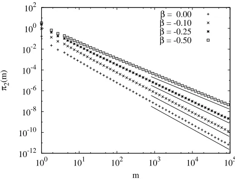
[image:6.612.321.558.55.235.2]β = 0.00 β = -0.10 β = -0.25 β = -0.50
FIG. 2: The variation ofπ2(m) withmis forβ=−0.5 (top curve),−0.25,−0.10,0 (bottom curve). The solid lines cor-respond to the exponent as predicted by CFR [see Eq. (14)]. Curves have been slightly shifted for clarity.
This perturbative argument demonstrates that sys-tems which are local at the mean-field level remain so for some time as one decreases the physical dimension into the diffusion-limited regime. It does not tell us much about whether locality holds by the time one reaches the next physically relevant, integer valued dimension below the critical dimension since this is presumably beyond the perturbative regime. In general, this is a difficult problem. The only case which we are aware of which can be handled analytically is the constant kernel (β = 0). It may be shown to be true ford >2 where mean field holds [16], ind= 2 due to a cancellation of logarithmic corrections [12] and ind <2 by an exact solution [18].
Lacking an analytic approach for other kernels, one must rely on numerical simulations to measure the value of σ for particular systems. We perform a systematic numerical investigation of locality in one dimension for several kernels in Sec. V C.
V. NUMERICAL SIMULATIONS OF CFR
A. Numerical measurements of CFR exponent
In this section, we present results of numerical simula-tions directly measuring the exponenthgiven in Eq. (14) It is in one dimension that the effects of fluctuations are the strongest. Hence, if the mean field scaling predicted by CFR is violated, then it will be violated in one dimen-sion too. For this reason, all the numerical results that we show will be monte carlo simulations for one dimensional lattices.
In our simulations we investigated the following repre-sentative kernels:
λ(m1, m2) = mβ1+m
β
10-16 10-14 10-12 10-10 10-8 10-6 10-4 10-2 100
100 101 102 103 104 105
π2
(m)
m
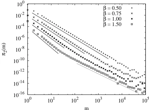
[image:7.612.322.557.52.227.2]β = 0.50 β = 0.75 β = 1.00 β = 1.50
FIG. 3: The variation of π2(m) with m for β = 0.50 (top curve), 0.75,1.00,1.50 (bottom curve). The solid lines corre-spond to the exponent as predicted by CFR [see Eq. (14)]. The dotted line corresponds to exponent forβ = 0. Curves have been slightly shifted for clarity.
λ(m1, m2) = (m1m2)β/2, (24)
λ(m1, m2) = max[m1, m2]νmin[m1, m2]µ, (25)
which we shall refer to as the additive, multiplicative and mixed kernels respectively. As far as the value ofhwas concerned, the results were identical for all three kernels. Hence, unless stated otherwise, our figures present results only for one of them, namely the additive kernel, Eq(23). What is convenient to measure in simulations is not
hN(m1)N(m2)i, but the quantity,
π2(m) =
Z ∞
m
dm1hN(m)N(m1)i. (26)
CFR predicts thatπ2(m) scales asπ2(m)∼m−2−β.
In Fig. 2, the variation of π2(m) with mis shown for
β= 0,−0.10,−0,25,−0,50. The solid lines are the CFR results. As can be seen, there is excellent agreement, confirming that CFR holds whenβ≤0. Fig. 3, shows the variation of π2(m) withm for β = 0.50,0.75,1.00,1.50.
The solid lines are the CFR results. The CFR exponent is obtained for small and intermediate masses but there is a clear cross-over to another behaviour at large masses. This can be understood as a finite size effect which we shall discuss in section V B.
At this point it is appropriate to make some comments on the correspondence with mean field theory. For the additive kernel, Eq(23), at the mean field level it is be-lieved [19] that β= 1.0 corresponds to the threshold for instantaneous gelation so that analytical understanding of the solutions of the Smoluchowski equation forβ >1 is very difficult. Notwithstanding the cross-over to another regime at large masses, it is very interesting that the CFR exponent is observed over some considerable range even for β >1. To the best of our knowledge, nothing
10-16 10-14 10-12 10-10 10-8 10-6 10-4 10-2 100
100 101 102 103 104 105
π2
(m)
m L = 100
L = 1000 L =10000
105
100 100
10-5
10-10
103 100 10-3
π2
(m) L
7/3
m L-2/3
FIG. 4: The lattice size dependence of π2(m, L) is shown for n = 3 and β = 1.5. The different lattice sizes are
L= 100,1000,10000. The crossover moves to the right with increasingL. Inset: The curves are scaled as in Eq. (27). The straight lines correspond to slopes−7/2 and−2.
is known about the behaviour of gelling kernels in the diffusion limited regime or in the presence of a monomer source. In this light, the results of Fig. 3 pose many in-teresting questions such as whether there is any remnant in the diffusion–limited regime of the catastrophic singu-larity which occurs in the mean–field equation atβ= 1.
B. Finite size effects
Let us consider why the lattice size should affect the CFR scaling. At this point it is useful to recall two things. Firstly, the recurrence property of random walks plays a crucial role in determining the statistics of aggregation in the diffusion limited regime. Due to recurrence, heavy particles develop “zones of exclusion” around them as they grow, resulting in strong anti-correlations between heavy particles. Secondly, recall that the CFR exponent quantifies the decreasing probability of two heavy parti-cles meeting each other. Due to the presence of zones of exclusion, this probability decreases faster for heavy particles than the product of one-point densities would suggest.
Although zones of exclusion grow larger as particles get heavier, in an infinite system there are always enough heavy particles to maintain the CFR scaling over all mass scales. In a finite system, however, these zones of exclu-sion become limited by the system size eventually. Once this happens, heavy particles start to meet each other more often than would be expected from CFR since thay can no longer grow their zones of exclusion any larger. Thus a finite size cross-over occurs and results in a shal-lower scaling as evident from Fig. 3. No such crossover occurs for the β < 0 cases shown in Fig. 2 since for
[image:7.612.56.297.55.233.2]reac-7
@ @@ β
ν
-0.250 -0.125 0.000 0.125 0.250 0.375 0.500
[image:8.612.320.560.55.241.2]-0.25 1.33 1.33 1.35 1.44 1.57 1.69 1.82 0.00 1.34 1.32 1.34 1.45 1.58 1.70 1.83 0.25 1.32 1.31 1.34 1.46 1.58 1.70 1.83 0.50 1.31 1.31 1.33 1.46 1.59 1.70 1.82
TABLE I: The numerical values of σ − h/2 are shown for different ν and β. The kernel used in λ(m1, m2) = max(m1, m2)νmin(m1, m2)µ. The errors in the values are
±0.02.
tive which acts to counterbalance the growth of zones of exclusion due to recurrence.
The argument above does not explain why finite size ef-fects should lead to a the scaling corresponding toβ= 0 indicated in Fig. 3. We suggest the following heuristic argument. For a finite system size,C(m1, m2) for ’large’
masses is contributed to by configurations consisting of two heavy particles which have been in the system for times ≫ L2, so that they are strongly-anticorrelated.
Hence these two particles effectively interact with each other at infinite rate, with effective diffusive jumps of the size equal to system size. HenceC(m1, m2) behaves
as if beta=0 at these masses. Since the mass flux is car-ried by the meetings of these super-heavy particles, it is presumably highly intermittent. It is then intuitive that the constant flux argument should fail to describe this regime.
Given that we expect to see CFR scaling for small masses andβ = 0 behaviour for large masses, we expect thatπ2(m, L) should have the form:
π2(m, L) =
1
L1+2/βf
m
L1/β
, β >0, (27)
where the scaling function f(x) varies asf(x)∼x−2−β
whenx→0 andf(x)∼m−2whenx≫1. The crossover
massmc is given bymβc ∼L, ormc∼L1/β.
In Fig. 4, we study the variation of π2(m, L) withm
for fixed β and differentL. Theβ value is chosen to be
β = 1.5. As expected from the preceeding discussion, the crossover point moves to the right with increasing
L. In the inset, the data is scaled according to Eq. (27) and excellent collapse is obtained. The large and smallx
behaviour of the scaling function behaves as predicted.
C. Numerical validation of locality criterion
As stressed in Sec. IV, aside from a couple of special cases we do not know whether the locality criterion is satisfied in one dimension or not. We now present nu-merical measurements of the exponent σ in Eq.(17) to address this issue. We choose our lattice size sufficiently large to avoid any question of the finite size effects dis-cussed in the previous section influencing the exponents.
10-12 10-10 10-8 10-6 10-4 10-2 100 102
100 101 102 103 104
π2
(m)
m β = 0; κ = 0.0 β = 0; κ = -0.5
100
10-2
10-4
10-6
104 102
100
〈
N(m)
〉
m
β=0;κ= 0.0
[image:8.612.51.301.58.132.2]β=0;κ=-0.5
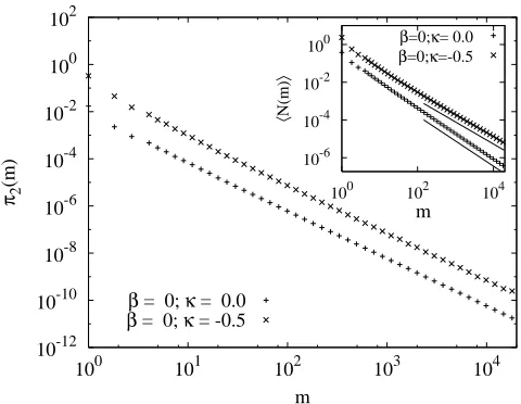
FIG. 5: The dependence on diffusion constant of ofπ2(m, L) is shown forn= 3 andβ= 0. The bottom curve corresponds to D(m) ∼ m0
[κ = 0] and the top curve corresponds to
D(m) ∼ m−1/2
[κ = −1/2]. The curves have same slope. Inset: The variation ofhN(m)iwithmis shown. There is a strong dependence onκ. The solid lines have slope (4 +κ)/3.
We use the mixed kernel, Eq.(25) so as to be able to vary
ν and µ independently. What is measured numerically ishN(m1)N(m2)iwhenm1 is kept fixed andm2≫m1.
ThenhN(m1)N(m2)i ∼mh/1 2+σm h/2−σ
2 . In our
simula-tions we keep m1 fixed at 5m0 and take m2 large and
measureσ−h/2. The results of a systematic set of nu-merical experiments are shown in Table I. What one sees is thatσ−h/2 is independent of β and dependent only onν. The numerics suggest that:
σ−h
2 = 4
3 + max[ν,0]. (28) If this is true, thenσ=−1/6+(ν−µ)/2 whenν >0, and
σ=−1/6−β/2 whenν <0. Comparing with the locality condition in Eq. (21), we see that it is always satisfied. Based on numerical evidence we therefore conclude that the spatially extended system is able to adapt itself to variations in the exponentsµand ν so that the locality criterion is always satisfied.
D. Lack of dependence on spatial transport mechanism
An important prediction of CFR is the lack of depen-dence on the diffusion constant. In Fig. 5, we show two sets of data for the same kernel but different diffusion constants. In one the diffusion constant is independent of mass. In the other it goes as D(m) ∝ m−1/2 such
that κ = −1/2. As can be seen, π2(m) scales exactly
VI. HIGHER ORDER AGGREGATION PROCESSES
Higher order aggregation processes may be considered where coalescence can only occur whenn−1>2 parti-cles meet at a single site. Although such processes have fewer physical applications than the binary case (n= 3), they have been suggested as an appropriate model of cer-tain polymeric reactions [20] and have received some
at-tention in the literature [10, 21, 22]. From a theoretical perspective, such systems provide an illustrative example of the breakdown of the CFR scaling due to a violation of the locality criterion. For these reasons, we consider the extension of the CFR argument to such systems.
Again, we will restrict ourselves to the case where the reaction rate λ(m1, . . . , mn−1) is a homogeneous
func-tion of its arguments of degree β. The Hopf equation corresponding to Eq.(5) is:
∂
∂t −D∇
2N(m) = Z ∞ 0
n−1 Y
i=1
dmiλ(m1, . . . , mn−1)
n−1 Y
i=1
N(mi)δ
"n−1 X
i=1
mi−m
#
−(n−1)
Z ∞
0 n−2 Y
i=1
dmiλ(m1, . . . , mn−2,m)N(m)
n−2 Y
i=1
N(mi) +
J
m0
δ(m−m0), (29)
The flux-carrying correlation function is the (n−1)-point correlation function denoted by
C(m1, . . . , mn−1) =hN(m1). . . N(mn−1)i, mi6=mj.
(30) By analogy with Eq.(8), we introduce a quantity
I(m1, . . . , mn−1;mn):
I(m1, . . . , mn−1;mn) =
λ(m1, . . . , mn−1)C(m1, . . . , mn−1)δ
"n−1 X
i=1
mi−mn
#
(31)
On taking average in Eq. (29), the diffusion term drops out. Then, form > m0we can write Eq. (29) as
∂hN(m)i
∂t =
Z ∞
0 n−1
Y
i=1
dmi
I(m1, . . . , mn−1;m)
− n−1 X
j=1
I(m1, . . . , mj−1, m, mj+1, . . . mn−1;mj)
(32)
The Zakharov transformations are:.
mi →
mmi
mj
, i6=j, (33)
mj → m
2
mj
, (34)
one for each of the n−1 negative integrals. They have Jacobians (m/mj)n. Looking for homogeneous solutions,
C(Λm1,Λm2, . . . ,Λmn−1) = ΛhC(m1, m2, . . . , mn−1)
(35) and using the homogeneity exponent ofλ, we obtain
0 =
Z ∞
0 n−1
Y
i=1
dmiI(m1, . . . , mn−1;m)
"
my−
n−1 X
i=1
myi
#
(36)
wherey=−h−β−n+1. We obtain a stationary solution whenh=−β−n. The uniqueness argument of Sec. III is easily extended to the case of n-ary interactions.
It is cumbersome to discuss in full generality locality for higher values ofn. Instead, we do a mean field analy-sis forn= 4 (three particles coalesce to form a new par-ticle) for the additive kernelλ(m1, m2, m3) =mβ1+m
β 2+
mβ3. In the mean field limit hN(m1)N(m2)N(m3)i ∼
(m1m2m3)h/3. When considering the collision integrals
as a function ofm1 (say whenm1→ ∞), there is a free
integral overm2. This integral being an integral over a
pure power law, will either diverge at∞or at 0. Hence the integrals are no longer finite and the locality con-dition will not be satisfied. Physically what happens is that three body collisions between three large particles are overwhelmed by three body collisions involving two large particles and one particle of very small mass. Thus the system behaves effectively asn= 3. One can get over this problem by introducing local kernels as discussed be-low.
We now present some numerical results forn= 4. We consider additive kernel withβ = 0,i.e,
λ(m1, m2, m3) = 1. (37)
and measure the quantity
π3(m) =
Z ∞
m
Z ∞
m
dm1dm2hN(m)N(m1)N(m2)i. (38)
which has a constant flux scaling ofπ3(m)∼m−2−β.
Forβ = 0, the upper critical dimension is one. Hence, by the argument above, the locality condition should be violated and we should get scaling corresponding ton= 3. In Fig. 6, we show the variation of π3(m) with m.
9
10-14 10-12 10-10 10-8 10-6 10-4 10-2 100 102
100 101 102 103 104 105
π3
(m)
m non-local
local
10-2
10-5
105 103 101
〈
N(m)
〉
m non-local
[image:10.612.57.297.56.238.2]local
FIG. 6: The variation ofπ3(m) withmis shown for the non lo-cal kernel Eq. (37) [bottom curve] and the lolo-cal kernel Eq. (39) [top curve]. The simulations are for n = 4. The solid lines have slope−3 and−2. Inset: the variation ofhN(m)i with
mis shown for the local and nonlocal kernels. Their scaling withmis independent of the kernel for largem.
m−3.0corresponding to scaling as predicted byβ = 0 and
n= 3.
To restore CFR, we consider a local kernel of the form
λ(m1, m2, m3) =g
m1
m2
g
m2
m3
g
m3
m1
, (39)
where the dimensionless function is chosen to be
g(x) = exp
x+1
x−2
(40)
This local kernel has the effect that it suppresses interac-tions between masses that are not of the same magnitude. The results ofπ3(m) for this local kernel is presented in
the top curve of Fig. 6. As can be seen, CFR is now obeyed. The inset of Fig. 6 shows that for both the local and non-local kernelshN(m)ihas the same scaling. this is again as expected because both forn= 3 andn= 4,
hN(m)i ∼m−4/3 modulo log corrections forn= 4.
VII. SUMMARY AND CONCLUSIONS
To summarise, we have performed an extensive theo-retical and numerical study of the applicability and con-sequences of the CFR argument introduced in [14] in the context of cluster-cluster aggregation with a monomer source. We have used a heuristic scaling argument and an exact anaylsis of the appropriate Hopf equation to show that the scaling of the flux-carrying correlation function in the stationary state is fixed by the fact that the ele-mentary coalescence interactions conserve mass. In the case of cluster-cluster aggregation, the flux carrying cor-relation function is proportional to the probability ofn−1
clusters coming together at the same point in space. It is thus not an esoteric object but is of direct physical significance.
The CFR scaling exponent is identical to that given by mean-field theory. It is thus independent of the physical dimension and independent of the details of the spatial transport mechanism. This latter fact we have demon-strated clearly with some numerical simulations of aggre-gation with mass-dependent diffusion rates. The impor-tance and non-triviality of the result lies in the fact that the flux-carrying correlation function exhibits the mean field scaling even in the diffusion limited regime where mean field theory fails to give correct answers for other correlation functions, in particular for the density. This runs counter to the usual intuition in interacting particle systems where it is canonical that statistics are domi-nated by diffusive fluctuations in low dimensions where mean field theory breaks down. We do not consider our result to be at odds with this canon. It is indeed the case that most statistical quantities measured in the diffusion limited regime will be fluctuation dominated. What we have shown is that there is a particular special correlation function which does not feel these fluctuations at all.
The usefulness of this result has already been demon-strated in our earlier work [11, 12] on constant kernel aggregation in low dimensions where it allowed us, taken together with a known exact result for the density, to prove multiscaling for the statistics of constant kernel ag-gregation in one dimension. Given the very direct phys-ical meaning of the flux-carrying correlation function in the aggregation context, it seems likely that other ap-plications will arise in concrete problems. At the very least, one can envisage using the result as a benchmark for numerical simulations of more complicated aggrega-tion problems, much as the 4/5-Law is used in validating numerical simulations of turbulence.
locality may violate CFR using a model kernel where the long range interactions may be tuned.
It is rare that a generic nonequilibrium system will be solvable as the model discussed in the paper. It could be that the distinction between driving and dissipation scales get fuzzy [23], or it could be that identifying the conserved quantity is a problem. In a recent paper [24],
we studied a model wherein the dissipation scale in not very well defined, and conjectured a CFR for such a model, even though it would not be expected apriori. The consequences of this conjecture was verified numerically. It would be of interest to clarify these observations the-oretically so that the results of the present article might be extended to an even wider class of models.
[1] S. Friedlander, Smoke, Dust, and Haze: Fundamentals of Aerosol Dynamics (Oxford University Press, Oxford, 2000), 2nd ed.
[2] V. Kontorovich, Physica D152–153, 676 (2001). [3] R. Drake, inTopics in Current Aerosol Research, edited
by G. Hidy and J. Brock (Pergamon Press, New York, 1972), vol. vol 3, part 2.
[4] R. Ziff, J. Stat. Phys.23, 241 (1980).
[5] S. N. Coppersmith, C. h Liu, S. Majumdar, O. Narayan, and T. A. Witten, Phys. Rev. E53, 4673 (1996). [6] P. S. Dodds and D. H. Rothman, Phys. Rev. E59, 4865
(1999).
[7] G. Huber, Physica A170, 463 (1991).
[8] D. Dhar, Studying Self-Organized Criticality with Ex-actly Solved Models, Preprint (1999), arXiv:cond-mat/9909009.
[9] D. J. Aldous, Bernoulli5, 3 (1999). [10] F. Leyvraz, Phys. Reports383, 95 (2003).
[11] C. Connaughton, R. Rajesh, and O. Zaboronski, Phys. Rev. Lett.94, 194503 (2005), cond-mat/0410114. [12] C. Connaughton, R. Rajesh, and O. Zaboronski, Physica
D222, 97 (2006), cond-mat/0510389.
[13] U. Frisch,Turbulence: The Legacy of A. N. Kolmogorov (Cambridge University Press, Cambridge, 1995). [14] C. Connaughton, R. Rajesh, and O. Zaboronski, Phys.
Rev. Lett.98, 080601 (2007), cond-mat/0607656. [15] V. Zakharov, V. Lvov, and G. Falkovich, Kolmogorov
Spectra of Turbulence (Springer-Verlag, Berlin, 1992). [16] C. Connaughton, R. Rajesh, and O. Zaboronski, Phys.
Rev. E69, 06114 (2004), cond-mat/0310063.
[17] A. Newell, S. Nazarenko, and L. Biven, Physica D 152-153, 520 (2001).
[18] R. Rajesh and S. N. Majumdar, Phys. Rev. E62, 3186 (2000).
[19] P. van Dongen, J. Phys. A: Math. Gen.20, 1889 (1987). [20] Y. Jiang, H. Gang, and M. BenKun, Phys. Rev. B41,
9424 (1990).
[21] P. Krapivsky, Phys. Rev. E49, 3233 (1994).
[22] Y. Jiang and H. Gang, Phys. Rev. B39, 4659 (1989). [23] L. P. Kadanoff, Rev. Mod. Phys.71, 435 (1999). [24] C. Connaughton, R. Rajesh, and O. Zaboronski, Physica

![FIG. 6: The variation of πhave slopewithm[top curve]. The simulations are forcal kernel Eq](https://thumb-us.123doks.com/thumbv2/123dok_us/9735745.474418/10.612.57.297.56.238/fig-variation-phave-slopewithm-curve-simulations-forcal-kernel.webp)
