Magneto encephalography (MEG) to image the brain’s role in the analgesic effects of Spinal Cord Stimulation (SCS)

(1)

Magneto-encephalography

(MEG) to image the brain’s role

in the analgesic effects of

Spinal Cord Stimulation (SCS)

Bart Witjes

9th_{of October 2018}

Medical Sensing and Stimulation

Technical Medicine, University of Twente

Graduation committee

Prof. Dr. ir. M.J.A.M. van Putten Drs. M.W.P.M. Lenders

Dr. ir. T. Heida Dr. ir. C.C. de Vos

(2)

1

Magneto-encephalography (MEG) to image the brain’s role in the

analgesic effects of Spinal Cord Stimulation (SCS)

Master Thesis

Bart Witjes

Technical Medicine

Medical Sensing and Stimulation

9th_{of October 2018}

Graduation committee:

Prof. Dr. ir. M.J.A.M. van Putten

Chair, external member

Drs. M.W.P.M. Lenders

Medical supervisor

Dr. ir. T. Heida

Technical supervisor

Dr. ir. C.C. de Vos

Additional member

Drs. N.S. Cramer Bornemann

(3)

2

Preface and acknowledgements

During my second M2 internship, I was first introduced to the neurosurgery department of the Medical Spectrum Twente. During that internship, I did EEG analysis of patients with a spinal cord stimulator and learned that I was really interested in this field of research. I was happy to be able to do my M3 internship at the same department, work with the same (and more) people and do further research in this field. The last year I have been working on this project with the goal to further exploring the cortical pain processing and the working mechanisms of spinal cord stimulation. Also, I was offered the opportunity to visit the MEG lab in Montreal and learned a lot about MEG data analysis. I really enjoyed working on this project, and I am really happy to be able to continue with the project after the completion of this thesis.

I would like to thank all my supervisors for their input and everyone that I have worked with for this project. A special thanks to Cecile de Vos, who has always made time to help me, showed me around in Montreal and introduced me to a lot of people, I really enjoyed working with her. I would also like to thank everyone in the MEG lab in Montreal for their help and teaching me how to use Brainstorm and their input for the project, specifically I would like to thank Elizabeth Bock and Martin Cousineau for answering all my questions. In addition, I want to thank everyone who participated in the study and everyone who helped with the measurements. I also like to thank the neurosurgeons and clinical staff of the MST neurosurgery department for giving me the opportunity to gain clinical experience. Last but not least, I would like to thank my girlfriend, Eline and my parents for their support.

(4)

3

Abstract

Background: Pain is a subjective experience and multiple factors play a role in the processing of pain. The network for the processing of pain, involving cortical and subcortical structures, has often been addressed in the neuroimaging of pain. Spinal cord stimulation (SCS) is used as a last-resort treatment for chronic neuropathic pain. Although there is plenty evidence that both, tonic and burst SCS, could be beneficial for neuropathic pain patients, the working mechanisms of SCS are still not fully understood. The goal of this study is to measure the neuronal activity in the pain processing brain areas and pathways involved in chronic neuropathic pain and assess how the different SCS settings affect the activity in these areas and pathways.

Methods: Resting-state magneto-encephalography (MEG) recordings were done in three groups of subjects: chronic pain patients (PC), subjects without pain (HC) and patients with SCS (PT). All subjects in the PT group evaluated one week of tonic, one week of burst and one week of placebo stimulation. The data analysis was two-fold: differences between HC and PC were analyzed, and the difference between different SCS settings were analyzed. For the HC and PC, the alpha power distribution was analyzed by computing a ratio of high theta power (7-9 Hz) and low alpha power (9-11 Hz). This was done at sensor level, and after source reconstruction. At source level, regions of interest (ROI) were defined and connectivity analysis was performed by computing the correlation and the coherence. For evaluation of the different SCS settings, the alpha power distribution was also analyzed at sensor and source level. The differences between SCS settings in power for the theta (4-7.5 Hz), alpha1 (8-10 Hz), alpha2 (10-12 Hz), beta1 (13-18 Hz), beta 2 (18.5-21 Hz) and beta3 (21.5-30 Hz) frequencies was also analyzed.

Results: Chronic pain patients showed significantly higher theta/alpha ratios predominantly at the right-sided sensors. Source reconstruction revealed significantly higher ratios in pain patients for the right insula, the mid-posterior and posterior cingulate cortex and the right S2. The coherence showed an increased connectivity between the right anterior insula and the right anterior S2. Comparing tonic to burst stimulation revealed a higher theta/alpha ratio during tonic stimulation for the temporal/occipital areas and the right insula. In addition, the somatosensory cortex and the parietal lobe showed increased alpha1 power for tonic stimulation. The power in the beta1 band for the somatosensory cortex and the parietal lobe was higher during burst stimulation.

(5)

4

List of abbreviations

(A)CC (Anterior) Cingulate cortex BPI Brief pain inventory

CPM Conditioned pain modulation CSF Cerebrospinal fluid

DBS Deep brain stimulation DMN Default mode network DNP Diabetic neuropathic pain

dSPM Dynamical Statistical Parametric Mapping ECD Equivalent current dipole

ECG Electrocardiogram EEG Electroencephalography

EOG Electrooculogram

EQ5D-5L EuroQ 5 dimensions questionnaire (5 levels) FBSS Failed back surgery syndrome

FDR False discovery rate

FM Fibromyalgia

FWER Family-wise error rate GABA Gamma-amino butyric acid

HADS Hospital anxiety and depression scale

HC Healthy Controls

HNP Herniated nucleus pulposus

IASP International association for the study of pain ISI Interstimulus interval

MCP Multiple comparisons problem MCS Motor cortex stimulation MEG Magneto-encephalography MNE Minimum norm estimates MRI Magnetic Resonance Imaging MSR Magnetically shielded room NRS Numeric rating scale

PC Pain Controls

PCA Principal component analysis PCS Pain catastrophizing scale PSD Power spectral density PT Patients (with SCS)

PVAQ Pain vigilance and awareness questionnaire ROI Region of interest

S1 Primary somatosensory cortex S2 Secondary somatosensory cortex SCS Spinal cord stimulation

(6)

5 SEP Somatosensory evoked potential

SQUID Superconducting quantum interference device SSP Signal-space projections

TCD Thalamocortical dysrhythmia VAS Visual analogue scale

(7)

6

Chapter 1: Background

1.1 Pain

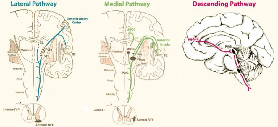
[image:9.612.71.541.341.557.2]

“Pain is an unpleasant sensory and emotional experience associated with actual or potential tissue damage, or described in terms of such damage.” [1] This is the definition of pain, given by the international association for the study of pain (IASP) and acknowledges the multidimensional character of pain perception. Pain is processed through at least three different pathways: the ascending medial pathway, the ascending lateral pathway and the descending inhibitory pathway (fig 1). The medial pathway modulates the motivational, affective components of pain. It is activated by C-fibers, runs to the mediodorsal and ventral posterolateral nuclei of the thalamus and subsequently connects to the anterior cingulate and anterior insula respectively. The lateral pathway modulates the discriminatory components of pain. It is activated by C, Aδ and Aβ fibers, runs to the ventral posterolateral nuclei of the thalamus and connects to the somatosensory cortex and parietal area. The descending pathway suppresses ongoing pain. It connects the pregenual anterior cingulate cortex to the periaqueductal gray and then runs to the somatosensory periphery [2, 3]. So, cortical and subcortical structures are involved in the perception and processing of pain. This network has been referred to as the ‘pain matrix’ and has often been addressed in the neuroimaging of pain [4].

Figure 1: Schematic overview of three pain processing pathways: the lateral, medial and descending pathways. The lateral pathway processes the discriminatory components of pain, the medial pathway processes the motivational, affective components of pain and the descending pathway suppresses ongoing pain. Figure from de Ridder et al. [5].

(10)

9 the sensation of pain due to a stimulus which is normally not painful (allodynia) [6]. Common treatment options of neuropathic pain are pharmacological options or, if possible, surgical intervention. However, these options do not always result in the desired pain relief.

1.2 Spinal Cord Stimulation

Spinal cord stimulation (SCS) is used as a treatment for chronic neuropathic pain, for example in the case of failed back surgery syndrome (FBSS) and diabetic neuropathic pain (DNP). Patients with FBSS still suffer from persistent neuropathic pain although they already had spinal surgery. This mostly involves lumbosacral spinal surgery for the treatment of spinal stenosis, with or without HNP [7]. DNP is caused by poor perfusion due to diabetes mellitus and is mostly presented as persistent pain in the feet and lower legs.

For SCS therapy, an electrode lead is placed in the epidural space over the dorsal columns of the spinal cord. A current is applied via this electrode, which results in pain relief in the dermatome innervated by the stimulated nerves. The precise working mechanism behind SCS is not completely understood, but there are several theories. The assumed main working mechanism is the gate control theory, which was proposed in 1965 by Melzack and Wall [8]. The gate control theory suggests that stimulation of the dorsal horn results in activation of the large Aβ-fibers, which blocks the pain signal that is transmitted by smaller Aδ and C fibers. The activation of the Aβ-fibers produces a tingling sensation (paresthesia) in the innervated dermatome, but ideally patients do not perceive the pain in that dermatome anymore [5, 9, 10]. SCS might work through antidromic activation of the ascending pathways, but could also work through orthodromic activation of the descending pathway. In addition, some animal studies suggest that the stimulation of A-fibers results in the release of gamma-amino butyric acid (GABA), which results in pain suppression at the spinal level by local interneurons [10].

Currently, there are two general stimulation settings used in SCS: tonic stimulation and burst stimulation. Conventional tonic stimulation is generally programmed with an amplitude between 2 and 15 mA, a pulse width between 0.1 and 0.5 ms and a frequency between 30 and 80 Hz [11, 12]. Nowadays, also high frequency tonic stimulation is used, with frequencies up to 10 kHz [13]. Burst stimulation generally has a lower amplitude and a larger pulse width compared with conventional tonic stimulation. For burst stimulation the pulses are delivered in packages (bursts) of five pulses, alternated with a resting period. The bursts are delivered with a frequency of 40 Hz, with the five pulses at 500 Hz [9]. Although conventional tonic stimulation is accompanied by paresthesia, both high frequency stimulation and burst stimulation can achieve pain relief without the occurrence of paresthesia.

1.3 Magneto-encephalography

(11)

10 synchronously and in parallel, directly [14]. MEG measures the activity of the same type of cells, but instead of measuring a potential difference between two electrodes, it measures the magnetic field that is evoked by large assemblies of neurons, which fire synchronously and in the same direction [14].

As the magnetic fields, generated by neuronal currents, are very small (of the order of several tens of femto Teslas), the MEG sensors have to be very sensitive. To acquire this sensitivity, the MEG scanner uses superconducting quantum interference devices (SQUIDs) to capture the cortical activity. Liquid helium is used to create the extremely cold environment that is necessary for super conduction. As the sensitivity of the sensors is very high, the MEG signal is easily contaminated with noise. To minimize the influence of noise, MEG measurements are conducted in a magnetically shielded room (MSR) and subjects should not have any form of magnetic metals in or on their body (for example, dental work).

Source localization is the principle whereby the source of the MEG signal is estimated. Source localization involves two main models: a forward model and an inverse model. The forward model consists of two parts: a source model, which explains how the neural electrical currents produce a magnetic field, and a volume conductor model, which explains how this magnetic field is transmitted through the tissues to the MEG sensors. A commonly used approach for the source model is the equivalent current dipole (ECD) approach, whereby multiple current dipoles represent post-synaptic electrophysiological activity of groups of neurons. A volume conductor model is then used to describe the electrical properties of the tissue and explain how the currents flow towards the MEG sensors. An advantage of MEG is that the magnetic fields are not affected by the cerebrospinal fluid (CSF) and the skull, whereas these factors do distort the EEG signal. Therefore, simplified volume conductor models can be used for MEG [14, 15].

The inverse model explains where the MEG signals are coming from. In the case of an ECD source model, we want to know which current dipoles produce which part of the MEG signal. However, we have a large number of current dipoles and a much smaller number of MEG sensors: this is called the inverse problem. Although there is no true solution to the inverse problem, there are multiple methods that approach a solution. An example of such an approach is the minimum norm estimate: this model minimizes the error between the source model and the recorded MEG signals [14, 15].

(12)

11

Chapter 2: Rationale

2.1 Spinal cord stimulation

During my previous internship at the neurosurgery department, we used EEG data to study the effect of SCS on the activity of the brain [16]. The goal of that internship was to examine whether the brain activity of chronic pain patients treated with SCS showed the same feature as previously described by Schulman et al. [17]: a slowing of the alpha frequencies towards the theta frequencies in chronic neuropathic pain patients. To quantify slowing of alpha frequencies, they defined a theta/alpha ratio as the power in the high theta frequency band (7-9 Hz) divided by the power in the low alpha band (9-11 Hz). They found an increased theta/alpha ratio for neuropathic pain subjects and failed SCS subjects, which was similar to the ratio of subjects with thalamocortical dysrhythmia (TCD) disorders. For successful SCS subjects however, the theta/alpha ratio was comparable with control subjects without pain. This caused the authors to believe the processing of pain works differently for subjects for whom SCS is not successful, compared to the subjects for whom SCS is successful. The main finding of my previous internship was in line with Schulman et al: patients, in whom SCS did not result in pain relief (subjects in pain), showed a relatively higher power in the theta frequency band and lower power in the alpha frequency band, than the control subjects without pain. However, these results were not statistically significant due to the limited number of subjects and the variation between subjects was very large. Schulman et al. reported on a limited number of subjects as well.

Another point of interest during my previous internship was the working mechanisms of two different stimulation settings; conventional tonic and burst stimulation. This was first studied by de Ridder et al. [5, 9]: during the trial stimulation phase of SCS, they tested one-week evaluation periods of tonic, burst and placebo (stimulator turned off) stimulation and recorded an EEG after each week of evaluation. They compared the EEGs of five subjects, wherefore the results showed more alpha activity in the dorsal anterior cingulate (which is a component of the medial pain pathway) during burst stimulation, compared to the other stimulation settings. Therefore, they suggested that burst stimulation modulates the lateral pathway and the inhibitory pathway, but also the medial pathway, whereas tonic stimulation only modulates the lateral pathway and the inhibitory pathway. During my previous internship I could not reproduce these results.

(13)

12

2.2 Chronic pain

Pain is a subjective experience and multiple factors play a role in the processing of pain. Already several different pain processing pathways and specific brain areas have been mentioned for their involvement in the processing of pain. In addition, it has been suggested that somatosensory processing is altered for chronic pain patients [19-21]. There are multiple studies whereby electrophysiological measures such as EEG have been used to try and objectify these alterations.

One of the reported alterations in EEG and MEG for chronic pain is slowing of the dominant rhythm [22]. For example, Schulman et al. described a shift of alpha peak frequency towards lower frequencies (theta) for chronic pain patients [17]. They compared resting state MEG recordings of subjects with deafferentation pain syndromes, subjects who had received SCS which resulted in pain relief and subjects who had received SCS which did not result in pain relief. They analyzed the shift of the alpha peak by computing a ratio of power in the high theta band (7-9 Hz) and power in the low alpha band (9-11 Hz) and found that deafferentation pain patients and patients for whom SCS was not successful, showed a larger shift from alpha frequencies towards theta frequencies. The shifting of the dominant (alpha) rhythm towards the theta frequencies is often described to thalamocortical dysrhythmia (TCD). TCD is described as a decreased inhibition of the thalamus, which causes an increased theta activity that reduces lateral inhibition, causes an increased gamma activity and therefore causes abnormal pain processing [17, 20, 22-24].

Possibly, the slowing of the dominant rhythm could be used to generate an electrophysiological marker of chronic pain. However, general slowing of the dominant rhythm has also been described in other neurological and psychiatric disorders (for example Alzheimer’s disease) and might not be specific enough [22, 25]. When more is known about the processing of chronic pain at the cortical level, it might also give better insights into the working mechanisms of SCS. At this moment, there is no clear, objective marker which describes the altered cortical activity of chronic pain patients yet. Such a marker would be useful to objectify, monitor or predict the effect of the treatment of pain, and to monitor or predict whether SCS in general or which stimulation settings in particular would be beneficial for an individual patient.

2.3 Aim of the study

The overarching goal of this project is to measure the neuronal activity in the brain areas and pathways that are involved in the processing of chronic neuropathic pain and assess how the different SCS settings affect the activity in these areas and pathways. As a first step to accomplish this goal, I proposed several objectives for this thesis:

• Study with MEG whether there is a shift in power from alpha frequencies towards theta frequencies for chronic pain patients compared to control subjects without pain

• Study which brain areas show this shifting of alpha frequencies towards theta frequencies, using a MEG source model.

(14)

13

• Study with MEG whether there is a difference in shifting of the alpha frequencies as a result of different SCS settings: tonic stimulation and burst stimulation.

• Study which brain areas show this shifting of alpha frequencies as a result of the different SCS settings, using a MEG source model.

• Study in which brain areas activity in specific frequency bands is altered as a result of the two different SCS settings, using a MEG source model.

(15)

14

Chapter 3: Methods

To achieve the goals described in 2.3, the study was divided into two parts. First, the differences in cortical activity between chronic pain patients and subjects without pain were analyzed. Second, the cortical activity of patients with a spinal cord stimulator was analyzed. After that, the results for the three different groups were compared. The data acquisition for all three groups was done in the same way, but the measurement protocol was different for the SCS patients as they evaluated three different stimulation settings.

3.1 Study groups

In total, three groups of subjects were recruited for this study; a group of chronic pain patients, a group of subjects without pain and a group of SCS patients. Because the overall goal is to study the effects of spinal cord stimulation, the groups of chronic pain patients and subjects without pain will be referred to as control groups. The three study groups and their inclusion criteria were as follows:

• Subjects without chronic pain (Healthy Controls, HC): no pain and no other neurological disease, but moderate, non-painful other medical conditions were not an exclusion criterion.

• Chronic pain patients (Pain Controls, PC): chronic neuropathic pain in the lower body part and preferably on a waiting list for a SCS implant. Subjects who also suffered from (severe) pain in another body part or another form of serious decline of general health, were excluded.

• SCS patients (Patients, PT): a SCS system which is capable of burst stimulation and already experienced more than three months of stimulation. Subjects who also suffered from (severe) pain in another body part or another form of serious decline of general health, were excluded.

3.2 Data acquisition

(16)

[image:16.612.108.501.134.425.2]

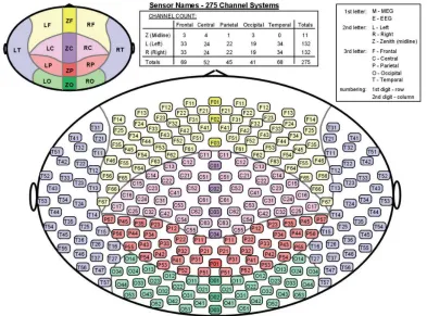
15 recording was made to capture the environmental noise. The noise recording was used for the noise cancellation in the process of source reconstruction (section 3.3.3).

Figure 2: The distribution of sensors in the helmet of the CTF 275-channel whole-head MEG system.

In the MEG, three conditions were tested; the resting state cortical activity, the cortical response to somatosensory evoked stimulation (somatosensory evoked potential, SEP) and the response to conditioned pain modulation (CPM). Because recording and cleaning the data (section 3.3.1) was very time-consuming, only the data of the first resting state recordings was analyzed for this thesis. For a better overview of the complete setup, the other conditions are explained briefly.

3.2.1 Measurement protocol HC and PC

(17)

16 results of the BPI were used to obtain the pain intensity for each subject. The pain intensity was expressed with the numeric rating scale (NRS), whereby 0 is no pain and 10 is the worst pain imaginable.

Resting state recordings: the participants were instructed to sit still, keep their eyes open, relax and to focus on a fixation cross. This recording lasted five minutes. The instructions and the fixation cross were presented to the subjects on a screen in the MSR. The presentation was made in Matlab, using the Psychophysics Toolbox extensions [26, 27].

SEP recordings: approximately 200 stimuli were applied to the median nerve (the first SEP recording) and the tibial nerve (the second SEP recording) with a randomly varying interstimulus interval (ISI) between 0.7 and 1.5 seconds. The stimuli were applied with a constant current electrical stimulator (Digitimer Ltd), which was programmed to deliver the stimuli with varying ISI using Matlab (The MathWorks, Massachusetts, USA). We used a pulse width of 200 microseconds and an amplitude level which was just high enough for eliciting a twitch. Subjects were instructed to silently count the number of stimuli, to ensure that the attention of the subjects was on the stimuli. After each SEP recording, we asked the subjects for the number of stimuli that they had counted, and they received feedback on their accuracy.

CPM recordings: the test consisted of three recordings, whereby each time 22 unpleasant stimuli were applied to the tibial nerve with a randomly varying ISI between 6 and 10 seconds. The stimuli consisted of a burst of 5 pulses each with a pulse width of 200 microseconds and with 5 milliseconds between each pulse. The amplitude of the stimuli was individually adjusted to the point where the subject indicated a pain score around 5 out of 10 (where 0 is no pain and 10 is the worst pain imaginable). During the first recording, only the stimuli were applied. During the second recording, the stimuli were applied in combination with an icepack on the left hand and forearm. After that, a third recording was done with the stimuli but without the icepack, to measure the extinction of the cold pressor test [28, 29].

3.2.2 Measurement protocol PT

To assess the effect of different stimulation settings on the cortical activity, the SCS patients underwent four MEG sessions. During the first session, a baseline recording was made with their own stimulation settings, after which the stimulation settings were changed to either tonic, burst or placebo stimulation. The type of stimulation was randomly chosen and neither the patient nor the researchers knew the type of stimulation. After this, the direct effects of the change of stimulation were recorded. One week later, the long-term effects of the change of stimulation were recorded with another MEG session (whereby the procedure of the first MEG session was repeated). Before each session, the subjects were asked to fill in the questionnaires (BPI, PCS, EQ5D-5L, HADS and PVAQ). From the BPI questionnaire, the NRS scores were used to indicate the pain intensity of the subjects.

(18)

17 and the CPM test. After this, the stimulation settings were changed to the next settings and another resting state recording of 5 minutes was done, followed by the two SEP recordings. During the fourth MEG session, the stimulation settings were not changed, therefore the session ended with a resting state recording only.

3.3 Data Analysis

The data analysis was performed with Brainstorm[30], which is documented freely and available for download online under the GNU general public license (http://neuroimage.usc.edu/brainstorm). All the steps that are explained in this chapter, are built-in options in Brainstorm. To learn about the possible steps and their technical background, I used the tutorials which are documented on their website. As mentioned before, these analyses were performed on the first resting state recording for every subject only.

Before any data analysis could be performed, the data had to be cleaned. Subsequently, the data analysis was performed in two parts. The first part of the data analysis consisted of analyzing the differences in cortical activity between pain and no pain, wherefore I looked at the following measures: the alpha power distribution; at sensor level, at source level and at specific brain regions of interest (which are known to be involved in pain processing). Also, I analyzed the connectivity between those specific areas by computing the correlation and the coherence between the specific areas. The differences were quantified using the statistical tests for MEG, available in Brainstorm. The second part consisted of analyzing the differences in cortical activity within the SCS group as a result of the different stimulation settings. For this part, also the alpha power distribution (at sensor level and at source level) was analyzed. To be able to compare the results with de Ridder et al. [5, 9], the differences in specific frequency bands for the different stimulation settings were analyzed.

3.3.1 Data cleaning

Because of the large number of artifacts, each resting state recording was first visually inspected and cleaned manually. The inspection was done in the time domain, and in the frequency domain by computing the power spectrum density (PSD) using Welch’s method with a 4 second window and 50% overlap. Individual or small groups of sensors that showed unexpectedly deviant behavior from their surrounding sensors, were marked as bad and excluded for further analysis.

Notch filters

(19)

18 Frequency filters

If deemed necessary, a bandpass filter was applied to remove low (< 1 Hz) and high (> 200 Hz) frequency noise. Low frequency noise could occur as a result of any form of metal in the subject’s body (for example, dental work); breathing causes these metals to generate a low frequency oscillation in the MEG signal. High frequency noise could occur as a result of muscle activity due to movement of the subjects. Muscle activity can be seen in the MEG signal at frequencies between 20 and 300 Hz [31], but the muscle activity lower than 200 Hz was not removed by using a lowpass filter, to prevent removing actual brain activity. The muscle activity below 200 Hz was removed differently, as will be explained in the next paragraph.

Principle component analysis (PCA)

The heart beat and eye movements cause artifacts in the MEG signal. The cardiac artifacts and the eye blinks, but also the muscle activity, were removed by using principal component analysis (PCA) [32, 33]. For the removal of the cardiac artifacts, the R-peaks in the ECG were detected and selected as an event. For the removal of the eye blinks, the peaks in the vertical EOG were selected as an eye blink event. If the recording was contaminated with multiple saccades, the horizontal EOG was used to mark the saccades as events. The events for muscle activity were selected either by automatic detection of data segments with an increased amplitude of frequencies between 40 and 240 Hz, or manually. After the detection of events, PCA was used to compute signal-space projections (SSPs) from these events. The resulting SSPs were topographies which represented the spatial distribution of the signal at the given events. For the SSPs which were similar to the artifact topography (for example, eye blinks occur at the most frontal sensors only), a linear projector was computed to remove this contribution from the signal. Artifacts whereby no sufficiently resembling SSP could be computed, were marked as ‘bad’ and these segments were excluded from further analysis.

3.3.2 Alpha power distribution: sensor level

The first measure that was calculated, was the measure described by Schulman et al. [17]; a shift of alpha frequency power, towards the lower theta frequencies due to neuropathic pain. A PSD was calculated for every sensor, using Welch’s method, with a 4 second window and 50% overlap. Subsequently, the power of the frequencies in the high theta band (7-9 Hz) and the power of the frequencies in the low alpha band (9-11 Hz) were extracted (for every sensor). The theta/alpha ratio was then calculated by dividing the power in the theta band by the power in the alpha band. To observe the group differences, an average ratio across all subjects in a group was calculated for each of the 275 sensors and visualized with a colormap in a schematic head: a theta/alpha ratio topography. As the final goal is to be able to distinguish between pain and no pain at an individual level, also the individual theta/alpha ratio topographies were computed.

(20)

19 3.3.3 Alpha power distribution: source level

For a better determination of the brain areas contributing to the MEG signal, the data was analyzed at source level. First, the MEG signal was linked to an MRI. If an individual MRI was available for the subject, the subject’s own anatomy was used. If there was no MRI available, the default ICBM152 MRI was used, and warped to the subject’s head, using the digitized head shape which was made before each recording. The MRI was used to perform cortical reconstruction and volumetric segmentation with the FreeSurfer image analysis suite, which is documented and freely available for download online (http://surfer.nmr.mgh.harvard.edu/). The result of the FreeSurfer software was the cortical surface extracted from the MRI [35]. This cortical surface was then imported into Brainstorm and downsampled to 15000 vertices. These vertices represent the number of dipoles to estimate during the source estimation process. To ensure a correct position of the head model in relation to the MEG helmet, 6 fiducial points (the nasion, the left- and right pre-auricular points, the anterior- and posterior commissure and an interhemispheric point) were marked in the MRI. Those points were then used to match with the anatomical points which were marked in the digitized head shape. The product of these steps was a cortical surface consisting of 15000 vertices, with a known position in relation to the MEG helmet.

The brain activity in the cortical surface was modeled in a current dipole model: one current dipole represents the post-synaptic electrophysiological activity of a group of neurons. To reduce computation time, the model was simplified, and the positions and orientations of the current dipoles were constrained. The positions of the current dipoles were set at the locations of the 15000 vertices, and the orientations were set perpendicularly with respect to the cortical surface (assuming that the measured fields are produced by apical dendrites, which are oriented normal to the surface) [15, 36]. The next step was to create a forward model; a model which explained how the MEG sensors capture the activity of the groups of neurons (the current dipoles). As MEG is less sensitive to the different head tissues (white and grey matter, cerebrospinal fluid, skull bone and skin) compared to EEG, the forward model was also simplified. For each MEG sensor, a sphere was estimated which represents the shape of the inner skull. In the end, the model consisted of overlapping spheres for each of the 275 MEG sensors [37].

(21)

20 resulted in source maps with values which were similar to z-scores and represented the measure of activity for each source.

The source maps were used to extract the alpha power distribution for every source. To reduce computation time, the PSD was only computed for the high theta band (7-9 Hz) and the low alpha band (9-11 Hz). Furthermore, the alpha power distribution was computed the same way as for the sensor level (described in 3.3.2).

3.3.4 Specific brain areas

The alpha power distribution was also computed for specific brain regions of interest (ROIs), which are known to be a part of the pain processing network [2, 3]. This was done to study whether there is a relation between the ROIs and the alpha power distribution. The areas that were studied more closely were: the prefrontal cortex, the insular cortex (anterior and posterior), the primary somatosensory cortex (S1), the secondary somatosensory cortex (S2, anterior and posterior) and the cingulate cortex (CC, anterior, mid-anterior, mid-posterior and posterior).

The source maps, that were obtained after the source reconstruction (see previous section), were used for analyzing the activity of the ROIs. The ROIs were defined by an assembly of sources on the cortical surface, which were situated in these brain areas. The Destrieux atlas, which is a parcellation scheme in FreeSurfer, was used to create these ROIs on the cortical surface [40, 41]. When the ROI from the Destrieux atlas did not completely cover the brain area, or cover more than the intended area, the ROI was modified in Brainstorm. The sources that represented the ROI are shown in appendix A. For each ROI, the average PSD across all sources in that ROI was calculated (again, for the high theta band (7-9 Hz) and the low alpha band (9-11 Hz) only). Subsequently the theta/alpha ratio was computed (section 3.3.2).

The same ROIs were used to analyze their connectivity. This was done by using two different measures; the correlation between the ROIs and the coherence between the ROIs. The correlation was computed for every subject by first computing the average time series for each ROI and then computing Pearson’s correlation coefficient between these 5-minute time series at zero lag. This resulted in a correlation coefficient, whereby a coefficient of -1 indicates a perfect negative linear relation between the two ROI and a coefficient of 1 indicates a perfect positive linear relation between the two ROI [42]. As the direction of the correlation was assumed to be of less importance and to improve the interpretability, the absolute values of the correlations were taken. The absolute correlation values per ROI were then averaged for each group. For the coherence, the PSD for each ROI was computed with a frequency resolution of 0.6 Hz. Subsequently, the PSDs of two ROIs (x and y) were compared by computing the magnitude squared coherence (COHxy). This was done by dividing the cross spectral density between the two ROIs (Sxy) by the PSDs of the two ROIs (Sxx and Syy) [42]:

𝐶𝑂𝐻𝑥𝑦(𝑓) = |𝐾𝑥𝑦(𝑓)| 2

= |𝑆𝑥𝑦(𝑓)|

2

(22)

21 The differences in coherence between the two groups were analyzed for the high theta band (7-9 Hz) and the low alpha band (9-11 Hz). As I selected a total of 16 ROIs (the mentioned brain areas for the left- and right hemisphere, the sources for the cingulate cortex were assumed to be in the middle), this resulted in averaged 16x16 connectivity matrices (for the correlation and for the coherence) for each group. To evaluate the differences, the connectivity matrices for the PC group were subtracted from the connectivity matrices for the HC group.

3.3.5 Statistical analysis

For performing statistical tests on the MEG data, I had to take into account the multiple comparisons problem (MCP). In the time domain for example, the data of two groups was compared for all 275 sensors at a lot of time points. This increases the chance of finding false positives; it increases the family-wise error rate (FWER). In Brainstorm, the nonparametric permutation test was used, because this method is more suitable to control for the FWER [43, 44].

For the nonparametric permutation test, first the trials of the HC group and the PC group were collected in a single set (resulting in 42 trials in total). Second, 21 trials were randomly selected from this set and put in subset 1, the rest was put in subset 2 (causing the HC and the PC to be mixed). Third, a two-tailed student’s t-test was performed between these subsets. Subsequently, the second and the third step were repeated 1000 times (1000 permutations) and a histogram was constructed of the test statistics. To reduce computation time, the Monte Carlo approach with only 1000 permutations was used. Therefore, this histogram only approximates the permutation distribution. The p-value was then determined by comparing the histogram and the observed test statistic (the t-test between the actual HC and PC). The p-value was the proportion of permutations that resulted in a larger test statistic than the observed statistic [43, 44].

To control for the FWER, the false discovery rate (FDR) correction was used, which corrected for the number of signals (the number of sensors or sources). The FDR corrected p-value represents the percentage of false positives of the significant values (without correction, the p-value represents false positive of all values) [45]. The corrected p-values were considered significant when they were smaller than 0.01.

Statistical analysis was performed only for the first part (comparing the HC and the PC). The permutation test was used to analyze the difference between the two groups for the following measures: the theta/alpha ratio topographies (section 3.3.2), the theta/alpha ratio for the sources and the theta/alpha ratio for the ROIs. For the second part (comparing the different stimulation settings of SCS), statistical analysis was not performed due to the low number of subjects.

3.3.6 Spinal cord stimulation

(23)

22 The alpha power distribution for the sensors (section 3.3.2) and the alpha power distribution for the sources (section 3.3.3) were computed and averaged for each stimulation setting (tonic, burst and placebo). To observe the differences between the stimulation settings, these three averages were subtracted from each other. This resulted in three figures for each measure: the differences between tonic and burst, between tonic and placebo, and between burst and placebo. Due to the low number of subjects, statistical analysis was not performed for this part of the analysis.

(24)

23

Chapter 4: Results

4.1 Pain vs. no pain

For the HC group, 21 subjects (8 females) were included. For the PC group, also 21 subjects (10 females) were included. The mean age and standard deviation (SD) were 47 ± 11 years old for the HC group and 48 ± 10 years old for the PC group. The NRS pain score was 0 ± 0 for the HC group and 5.5 ± 2.4 for the PC group. From the PC group, 38% suffered from pain in both (left and right) legs, 33% suffered from pain in their left leg (and not their right), 14% suffered from pain in their right leg and 14% suffered from pain in their back only.

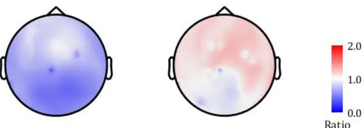
The results for the average theta/alpha ratio at each sensor for both groups are shown in figure 3. The ratio topography for the HC (left) showed ratios primarily below 1, which means that there is more power in the 9-11 Hz frequency band than in the 7-9 Hz frequency band. The ratio topography for the PC (right) showed ratios primarily above 1, meaning more power in the 7-9 Hz band than in the 9-11 Hz frequency band.

Figure 3: The theta/alpha ratio for each of the 275 sensors. The ratio topographies are shown for (left) the healthy controls and (right) the pain controls. The values represented in the figure are the theta/alpha ratios, a higher ratio means more power in the 7-9 Hz frequency band and a lower ratio means more power in the 9-11 Hz frequency band.

[image:24.612.129.494.354.483.2]

(25)

[image:25.612.206.405.79.217.2]

24 Figure 4: The results for a permutation t-test between average (sensor level) theta/alpha ratios for the healthy controls (HC) and the average (sensor level) theta/alpha ratios for the pain controls (PC). The values represented in the figure are t-values based on a significance level of p < 0.01, a high t-value means a higher ratio for the HC and a low t-value means a higher ratio for the PC. The results were false discovery rate (FDR) corrected for the number of sensors.

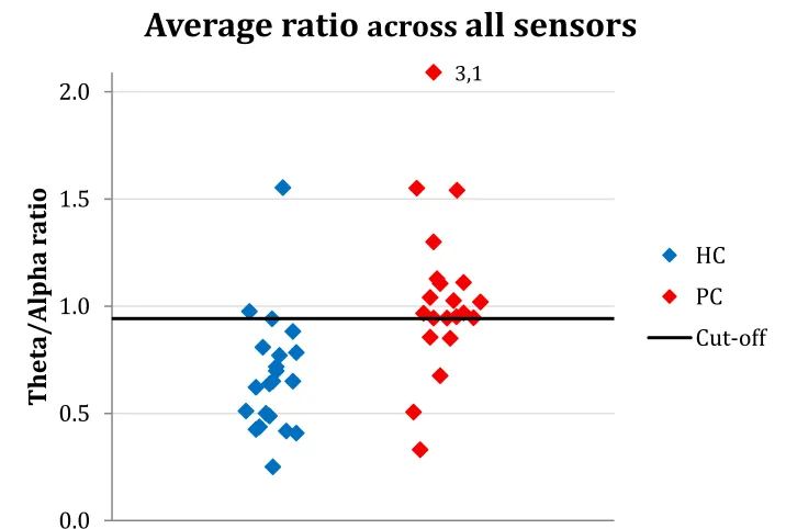
The individual ratio topographies (shown in appendix B.1) revealed that the topography could almost distinguish between HC and PC at the individual level, except for some outliers. The same individual differences were also visible in the theta/alpha ratio averaged across the whole head (fig. 5). The ROC-curve (appendix B.2) showed a cut-off value of 0.94, whereby chronic pain patients were detected with a sensitivity of 76% and a specificity of 91%.

Figure 5: The average ratio across all sensor for each subject. Subjects in the healthy control (HC) group are shown in blue and subjects in the pain control (PC) group are shown in red. The black line indicates the cut-off value (determined with a ROC curve) to distinguish between HC and PC.

3,1

0.0 0.5 1.0 1.5 2.0

Thet

a/

A

lp

ha

r

at

io

Average ratio

across

all sensors

[image:25.612.128.486.379.620.2]

(26)

25 4.1.2 Alpha power distribution: source level

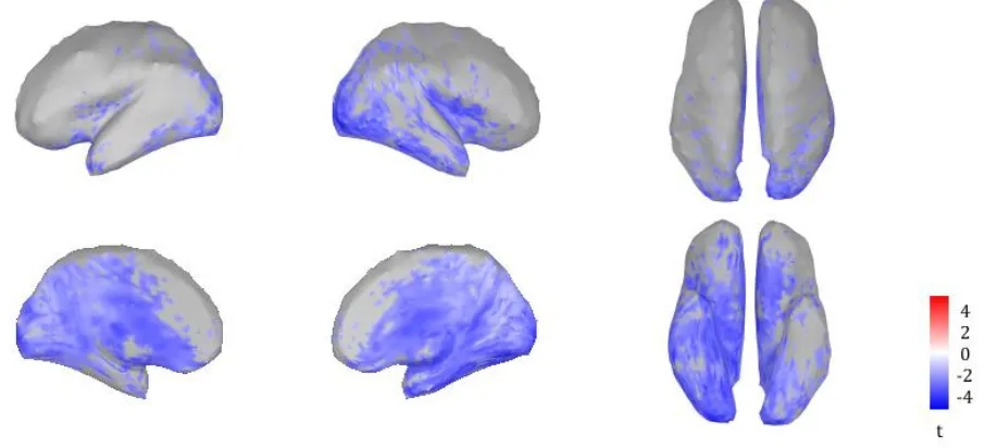
The differences between the two groups at source level are shown in figure 6. Sources which lighted up blue, showed a significantly higher theta/alpha ratio for the PC group (p < 0.01). The areas which showed the largest differences, were the insula (primarily the right insula), the cingulate cortex and the right temporal/occipital cortex.

Figure 6: The results for a permutation t-test between the average (source level) theta/alpha ratios for the healthy controls and the average (source level) theta/alpha ratios for the pain controls. The results were false discovery rate (FDR) corrected for the number of sources. The values represented in the figure are t-values based on a significance level of p < 0.01. The areas which showed the largest differences between the two groups, were the insula (primarily the right insula), the cingulate cortex and the right temporal/occipital cortex.

4.1.3 Specific brain areas

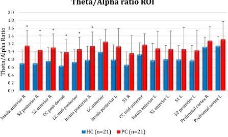
[image:26.612.85.538.164.370.2]

(27)

[image:27.612.85.532.85.355.2]

26 Figure 7: The average theta/alpha ratio in each region of interest (ROI) for the two groups, the error bars represent the standard deviation. The healthy controls (HC) are shown in blue and the pain controls (PC) are shown in red. The ROI with the most significant difference is shown on the left and the ROI with the least significant difference is shown on the right (p values were obtained by performing the permutation t-test). L = left, R = right, CC = cingulate cortex, S1 = primary somatosensory cortex, S2 = secondary somatosensory cortex, * = p < 0.01.

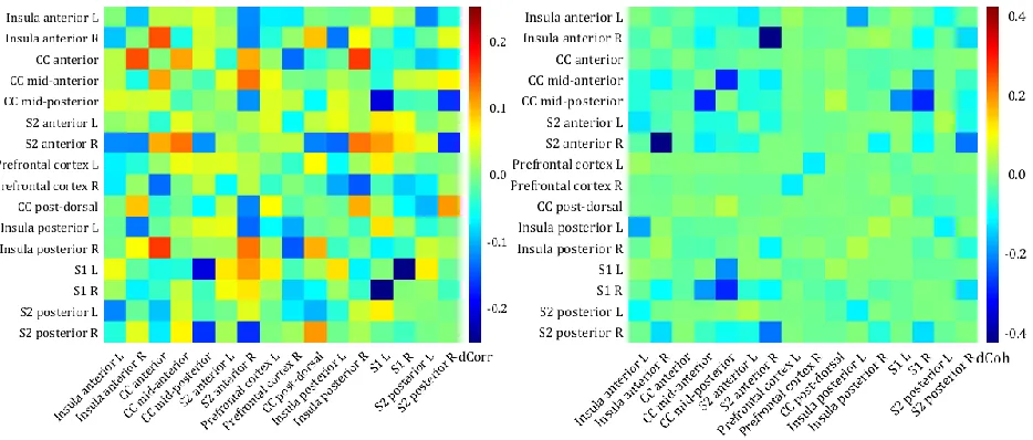
The connectivity matrices (correlation and coherence) for the differences between the HC and the PC for each ROI are shownin figure 8. The correlation values between the ROIs were generally low for both, the HC and the PC (appendix C.1) and therefore the differences between those two groups were only small. This is shown in figure 8 (left): a positive value means that the correlation or coherence between the two ROIs was larger for the HC and a negative value means that the correlation or coherence between the two ROIs was larger for the PC. The largest difference in correlation between the two groups was about 0.3 and found between the right S1 and the left S1: the correlation between those areas is larger for the PC than for the HC.

The coherence values between the ROIs showed a more distinct difference in connectivity between the two groups than the correlation values. The difference in coherence for the high theta band (7-9 Hz) and the low alpha band (9-11 Hz) show a similar connectivity pattern between the ROIs, however the coherence values were higher for the high theta band (appendix C.2). The largest difference in coherence (fig 8, right) between the two groups for the high theta band was found between the right anterior S2 and the right anterior insula: the coherence between those areas was about 0.5 for the PC and about 0.1 for the HC (appendix C.3). In the theta frequency band, there were also clear differences in coherence between the two groups for the different ROIs within the cingulate cortex and for the cingulate cortex and the S1: the coherence values between those areas were higher for the PC than for the HC.

* * * * * * 0.0 0.2 0.4 0.6 0.8 1.0 1.2 1.4 1.6 1.8 2.0

Th

et

a/Alpha R

at

io

Theta/Alpha ratio ROI

(28)

27 Figure 8: The differences in connectivity between the two groups, with (left) the difference between the correlation (within the regions of interest) of the healthy controls (HC) and the pain controls (PC) and (right) the difference between the coherence of the HC and the PC for the high theta band (7-9 Hz). The values are difference in correlation (left) or coherence (right) between the HC and PC, a positive value means a higher correlation/coherence between the two ROIs for the HC and a negative value means a higher correlation/coherence between the two ROIs for the PC. Note that the colorbars are scaled differently for the two matrices. L = left, R = right, CC = cingulate cortex, S1 = primary somatosensory cortex, S2 = secondary somatosensory cortex.

4.2 Spinal cord stimulation

For the PT group, 9 subjects (3 females) were included. The mean age for this group was 54 ± 10 years old. The mean reported NRS was 4.1 ± 3.0 after one week of tonic stimulation, 3.9 ± 2.1 after one week of burst stimulation and 5.4 ± 2.4 after one week of placebo stimulation. Five of the patients suffered from pain on their right side of the body, three on their left side and 1 suffered from pain on both sides.

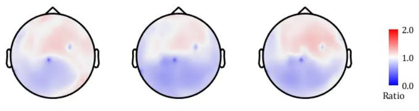
[image:28.612.76.543.102.301.2]

(29)

[image:29.612.97.516.77.188.2]

28 Figure 9: The average theta/alpha topographies (from left to right) after one week of tonic stimulation, one week of burst stimulation and one week of placebo stimulation.

The individual theta/alpha ratios averaged across the whole head seemed to be distributed similarly for each of the three settings (appendix D). The whole-head ratio averaged over the 9 subjects showed a ratio of 0.97 ± 0.30 for tonic stimulation, 0.88 ± 0.21 for burst stimulation and 0.94 ± 0.26 for placebo stimulation.

4.2.2 Alpha power distribution: source level

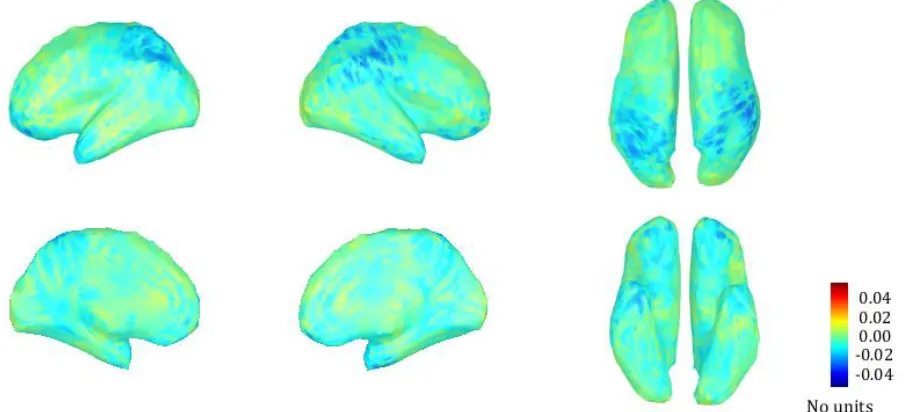
The differences in theta/alpha ratio between tonic stimulation and burst stimulation at source level are shown in figure 10. A positive difference (red) means a higher ratio during tonic stimulation and a negative difference (blue) means a higher ratio during burst stimulation. Especially the right temporal and occipital areas, but also the insula showed a higher ratio during tonic stimulation. The largest difference was seen in a small left frontal area, where the ratio was higher during tonic stimulation.

[image:29.612.84.537.446.656.2]

(30)

29 The differences in theta/alpha ratio between tonic stimulation and placebo stimulation are shown in appendix E.1. The largest (positive) difference was again observed in the frontal area of the left hemisphere, where the ratio was higher during tonic stimulation. The differences in theta/alpha ratio between burst stimulation and placebo stimulation (appendix E.2) did not reveal one specific area with a larger difference than other areas. Overall, the ratio was higher for placebo stimulation compared to burst stimulation, whereby the right hemisphere showed this difference more clearly than the left hemisphere.

4.2.3 Specific frequency bands

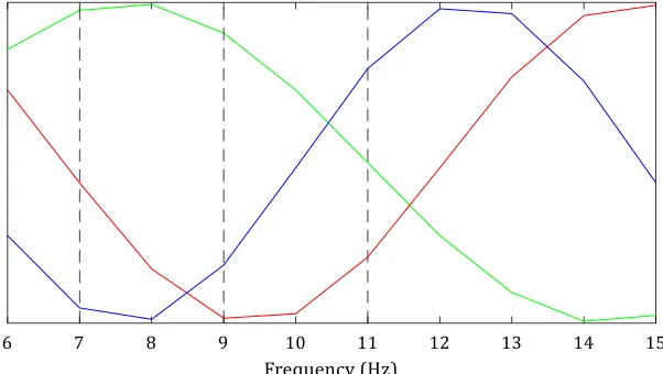
The comparison of the specific frequency bands (theta, alpha1, alpha2, beta1, beta2 and beta3) between the three different stimulation settings revealed the largest differences in the alpha1 band (8-10 Hz) and the beta1 band (13-18 Hz) when comparing tonic stimulation to burst stimulation. The somatosensory cortex and the parietal lobe showed increased alpha1 power during tonic stimulation, compared to burst stimulation (fig 11). The difference in alpha1 power was maximally 0.04 (unitless), which represented about 10% difference between the two settings, as the maximum alpha1 power for both tonic and burst stimulation was about 0.3 (appendix F.1). The effect of increased alpha1 power was also visible when comparing tonic stimulation to placebo stimulation, but not when comparing burst stimulation to placebo stimulation (appendix F.2).

On the contrary, the power in the beta1 band for the somatosensory cortex and the parietal lobe was higher during burst stimulation, compared to tonic stimulation (fig 12). Although the figures showed the same scales, the difference in beta1 power was larger than the difference in alpha1 power: the maximum power for both tonic and burst stimulation was about 0.15 (unitless), therefore the value of 0.04 represented about 25% difference between the two settings. When comparing burst stimulation to placebo stimulation, the beta1 power for these same areas was also higher, but the comparison between tonic and placebo stimulation did not reveal a clear difference (appendix F.3). Note however that these differences are between the means of 9 subjects, the individual results varied as did the effect of the three stimulation settings on their pain perception.

(31)

[image:31.612.82.537.78.283.2]

30 Figure 11: The difference in mean relative power in the alpha1 frequency band (8-10 Hz) between tonic stimulation and burst stimulation for every source. The positive values indicate more power in the alpha1 band during tonic stimulation, compared to burst stimulation. Especially the right hemisphere shows more alpha1 power in the somatosensory cortex and the parietal lobe during tonic stimulation.

[image:31.612.84.536.355.561.2]

(32)

31

Chapter 5: Discussion

5.1 Main findings

Comparing between chronic pain patients and healthy, pain-free control subjects, we found that the alpha power distribution is significantly different between the two groups: the chronic pain patients showed higher theta/alpha ratios for several brain areas, indicative for slowing of the alpha frequencies. In the regions of interest, this difference in alpha power distribution was mainly observed in the right insula, the mid-posterior and posterior cingulate cortex and the right secondary somatosensory cortex. The coherence for the high theta frequencies between the right anterior insula and the right anterior S2 was much larger in the PC group, compared to the HC group. The comparison between tonic and burst stimulation showed a higher theta/alpha ratio during tonic stimulation for the temporal/occipital areas and the right insula. Furthermore, there were differences in power in the alpha1 and beta1 frequency bands in the somatosensory cortex and the parietal lobe between tonic and burst stimulation.

5.2 Thalamocortical dysrhythmia

5.2.1 Pain vs no pain

The theta/alpha ratio was significantly higher in PC group, compared to HC group. This higher ratio indicates that the peak in alpha frequencies is shifted towards the (lower) theta frequencies in patients with chronic pain. The increased ratio could also be caused by an increased power in theta frequencies, which has been reported in other literature. In a review about EEG patterns in chronic pain by Pinheiro et al, four of the six studies found an increased theta frequency power for the chronic pain subjects [20]. The increased theta power could be the result of a decreased inhibition of the thalamus. The slower theta waves reduce the lateral inhibition, which could cause increased gamma activity in the areas that surround the areas which show an increased theta activity. This is called thalamocortical dysrhythmia (TCD) and has been associated with multiple neurological and psychiatric disorders, amongst which chronic pain [17, 20, 22-24]. The theta/alpha ratio might reflect this phenomenon in our chronic pain patients as well.

In our source model, the increase in theta/alpha ratio seemed to originate from sources deeper than the cortex and spread into multiple cortical areas. We expected that this source could very well be the thalamus and to test this hypothesis, we incorporated the thalamus into our original source model (appendix E.3). That extended model indeed projected a vast part of the increased theta/alpha ratio in the thalamus. However, caution has to be taken when interpreting this finding, as more research is needed to confirm that MEG is indeed capable of detecting signals which originate in the thalamus [46]. Nevertheless, these results and the previous findings in literature, strongly suggest an alteration in thalamic behavior because of chronic pain.

(33)

32 hemisphere. This has also been reported in literature: Pauli et al. found that pain sensitivity was associated with an increased right hemispheric activity [47] and Lugo et al. suggested that pain intensity perception is lateralized to the right hemisphere [48]. Also, the right insula is known to play a more significant role in attentional processes than the left insula [3, 49]. Another explanation for the larger differences in theta/alpha ratio on the right side is that TCD is mainly visible in the right hemisphere.

The average theta/alpha ratio across the whole head seemed to be able to distinguish quite accurately between the HC and PC. Especially the specificity (91%) was high for this method; most HC were correctly classified. The PC however showed a larger variation causing a sensitivity of 76%. The cut-off value could be decreased to obtain a larger sensitivity, as we could argue that the sensitivity is more important. Also, there are some clear outliers; the overall ratio of 3.1 for example, is clearly deviant from the other values and therefore has a larger impact on the cut-off value. Possibly, an explanation for the outliers can be found in the questionnaires (for example pain duration or peak pain intensity). The results from the questionnaires, but also the results from the other measures described in this thesis, could be incorporated in a more advanced model to improve the classifier. For this, a larger number of subjects would be desirable as well.

5.2.2 Spinal cord stimulation

The theta/alpha ratios at sensor level were slightly lower during burst SCS than during tonic or placebo stimulation. Also, the difference in theta/alpha ratio at source level between tonic and burst stimulation looks similar to the difference between chronic pain patients and healthy controls, except for the cingulate cortex (the CC shows comparable ratios for tonic and burst stimulation). Apart from the finding in the cingulate cortex, this could suggest that tonic stimulation does not affect TCD, but burst stimulation does or does to a larger extent. This might also be reflected in the pain scores; after one week of burst stimulation, the patients indicated lower pain scores on average. However, the differences in theta/alpha ratio and in the pain scores between the different stimulation settings were only small and there was variation between the subjects. With a larger number of subjects in the PT group, we would be able to group responders and non-responders to a certain stimulation setting, after which we expect to see clearer differences.

(34)

33 the thalamus, the primary motor cortex, the CC, the S1 and S2 and the insula. Apart from the motor cortex, these same areas also showed an increased theta/alpha ratio (the S1 to a lesser extent) when comparing our PC to HC.

The cingulate cortex, specifically the anterior cingulate cortex, has also been a target for cortex stimulation [52]. Boccard et al. performed deep brain stimulation (DBS) in the ACC for 16 neuropathic pain patients, of which 11 subjects were included for analysis. They showed an overall improvement of visual analogue scale (VAS) scores [53]. Also, Spooner et al. presented a case study whereby they implanted DBS in a patient with neuropathic pain, they also reported better pain control after implantation [54]. Another form of cortex stimulation as a treatment of chronic pain is motor cortex stimulation (MCS). Although the precise working mechanism of MCS is unclear, MCS is believed to modulate pathologic hyperactivity of thalamic relay nuclei. The success rates for MCS were higher for facial pain (68%) than for central pain (54%) [55]. This literature shows that modulation of pain processing areas such as the motor cortex and the ACC is able to reduce pain in some chronic pain patients. Possibly, SCS works also through modulation of these (or other pain processing) brain areas, but by activating or deactivating the pain processing pathways through the spinal cord.

5.3 Connectivity measures

Differences in connectivity between the HC and the PC were mainly found in the coherence. The maximum coherence was found for the frequencies below 1.5 Hz. Since a large part of the PC had artifacts below 1 Hz, a 1 Hz high pass filter was applied for these subjects. Therefore, the coherence below 1 Hz is not expected to be reliable. The frequency band that showed the highest coherence after the frequencies below 1.5 Hz, was the high theta frequency band (7-9 Hz). Since this frequency band and the low alpha frequency band (9-11 Hz) were the main frequencies of interest, only these frequency bands were shown. The frequency resolution that was used for the coherence matrices (0.6 Hz) was different from the frequency resolution that was used for the other measures (0.25 Hz, for the alpha power distribution and the specific frequency bands). The reason for this was to reduce the computational effort; a higher frequency resolution caused the process to reach out of memory. A higher frequency resolution would however be desirable, since the width of the frequency bands of interest was only 2 Hz.

(35)

34 Several studies have shown that the insula is involved in the processing of pain (amongst other psychological functions), specifically the affective/motivational component of pain [56, 57]. The insula has for example been mentioned for its involvement in pain processing for patients with fibromyalgia (FM): Hsiao et al. reported a decreased connectivity between the bilateral insula and the default mode network (DMN) for FM patients [58], Choe et al. reported a decreased connectivity within the DMN for FM patients [59] and Ichesco et al. reported an increased connectivity between the right insula and the CC for FM patients, but an increased connectivity between the left insula and the CC for controls [60]. So, there is literature which also shows an increased connectivity between the right insula and the other brain areas (involved in the processing of pain) for chronic pain patients, but there is also literature which suggests the opposite: that connectivity is decreased for chronic pain patients. Because the exact relation of the insula with other pain processing areas is still debated, this area and its connectivity with other ROI should be further explored with other connectivity measures.

We only found a difference in connectivity for the right insula, not for the left insula. Besides the study of Ichesco at al., there are other studies that have reported that the right insula is more important in the processing of pain than the left insula [3, 49, 60]. For example, Cauda et al. also found a stronger connectivity between the right insula and the areas associated with attentional processes (such as the ACC and the thalamus) than the left insula. Our findings and the literature suggest that the right insula is more important in the processing of pain than the left insula.

The correlation values showed very little difference between the two groups. Although both measures (correlation and coherence) were used to describe a relation between ROIs, the correlation values indicate a relation between areas in the time domain, where the coherence values indicate a relation between areas in the frequency domain. The correlation was computed with the assumption that the time lag between two ROIs was 0. This might not be entirely accurate, because the distance between two ROIs might cause a small lag in response. Also, the correlation values were averaged across the five-minute recordings, negative correlation values might have cancelled out positive correlation values, resulting in lower values than the coherence values. In order to reduce these effects, I also computed the maximum correlation across the five-minute recordings (appendix C.4). This however did not show larger differences than the mean correlations did. In addition, taking the maximum coherence across five minutes, is more sensitive to sudden non-physiological changes in the time signal. Because of these disadvantages, the correlation might therefore be a suboptimal measure for describing the connectivity in this case.

5.4 Specific frequency bands

(36)

35 during burst stimulation (in none of the frequency bands). The alpha1 power increase in the somatosensory cortex during tonic stimulation could be the result of the paresthesia, caused by tonic stimulation. This explanation was further supported after comparing tonic and placebo stimulation, and burst and placebo stimulation. The difference was also visible between tonic and placebo, but not between burst and placebo (where neither of the two causes paresthesia). Overall, our results do not show such a clear difference between tonic and burst stimulation to suggest that the two stimulation modes work through different pathways. It seems more likely that both, the tonic and the burst stimulation work through the concept of the gate control theory: the large Aβ-fibers block the pain signals of the smaller Aδ and C-Aβ-fibers but cause perceived sensations, whereas burst stimulation modulates the Aβ-fibers below the paresthesia threshold [9].

When comparing tonic stimulation and burst stimulation, a difference was also found in the beta1 frequency band, again for the somatosensory cortex. Although alpha1 power was higher during tonic stimulation in this area, beta1 power was higher during burst stimulation. The comparison between tonic and placebo stimulation did not reveal clear differences in beta1 activity, indicating that the beta1 power is increased during burst stimulation only. This suggests that both SCS settings are processed in the somatosensory cortex, whereby tonic stimulation causes alpha1 oscillations and burst stimulation causes beta1 oscillations. However, we do not have an explanation for this yet and further analysis with a larger number of subjects is needed to explore this finding.

The prefrontal cortex showed an increased theta power when comparing tonic to burst stimulation. As this difference was also visible between tonic and placebo, but not during burst and placebo, this difference could be caused by the tonic stimulation. This increased theta power was also reflected in the theta/alpha ratio; the ratio was higher for a small area of the prefrontal cortex when comparing tonic versus burst stimulation. Although other areas of the prefrontal cortex (such as the dorsolateral prefrontal cortex) have been reported to be involved in the processing of pain [9, 20], this small prefrontal area has not been reported yet in association with chronic pain. The data has been cleaned of eye blinks, but the location and the frequency of this difference could also originate from remaining eye movements. The source models of the individual subjects revealed that the theta power in the prefrontal cortex was higher during tonic stimulation (compared to burst) in three of the nine subjects. These three subjects might have had more eye movements during the recording, but it is unlikely that they only showed more eye movements during tonic stimulation, and less during burst stimulation. A larger number of subjects and extended data analysis is necessary to further explore this finding.