Caching in 5g networks

Caching in 5g networks

June 30, 2017

Ruben de Baaij

Jasper Goseling, Berksan Serbetci University of Twente

Abstract

Efficient ways of caching, saving files in local devices, is becoming more important. Especially with the upcoming 5g network. In this paper a way of distributing files over networks of caches is modeled and analyzed.

1.

I

ntroduction

Internet traffic becomes more and more busy every year. More files are being requested and shared constantly. The existing digital infras-tructure is struggling to keep up, and with the upcoming 5g network the demand of files in-creases even more. This is why a lot of research is going on to find new ways of transferring files. One of the methods to deal with the huge amount of file requests is the use of caches.

Caching is temporarily storing much re-quested data inside a memory devices called caches. When a file is requested it will be an-swered by a cache in which the file is stored, it will send the file to the user that requested it. This is faster than getting the file from the original server. Saving files in caches is a way to cut out a lot of internet traffic and more file requests can be answered.

Caches, also called base stations (BS), can be located anywhere around a user. Often a user is able to connect to multiple caches in the area. By an efficient distribution of files over the caches these multiple caches in range can be taken advantage of. There is no need to store the same file in every cache a user can connect to. It is enough to answer the request when a file is stored in just one of the caches in the area.

To find such a distribution of files a lot of questions come up. Which files have to be stored in which cache? In this paper the prob-ability that a request cannot be answered will be minimized. So the probability a user will recieve the file he requests will be optimized.

2.

T

he

M

odel

To find the optimal distribution of Jfiles over Ncaches the following function f(B)is used as an objective function in a mixed integer opti-mization system. The function gives the proba-bility a users’ file request is not answered using the file distribution matrixB.

The vector arepresents the probabilities a file is requested. These probabilities are gener-ated using a zipf distribution (1) with parame-terγ.

aj= j−γ J ∑ j=1

j−γ

(1)

The vectorprepresents the probabilities of a user being in an area where he can connect to the caches ins. Θis the set of all the combi-nations of caches a user can be in range of at once.

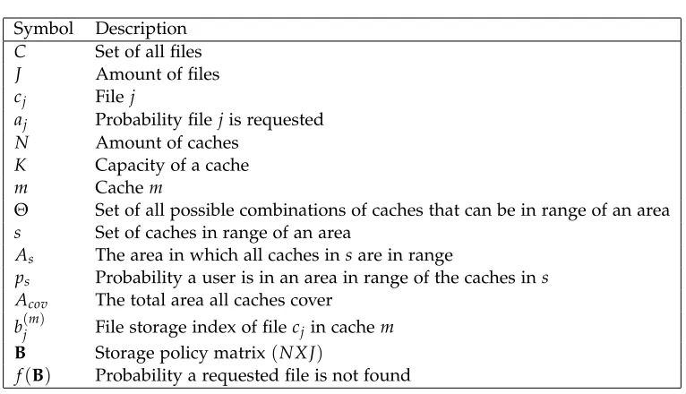
Furthermoreb(_jm)indicates if filejis stored in cachem. It equals 1 if the file is saved, and 0 if it is not saved. These indicators are stored in theN−by−Jdistribution matrixB. In table 1 of the appendix an overview of the defined variables is given.

f(B)=

J ∑ j=1

aj ∑ s∈Θpsm∏∈s

(1−b(_jm)) (2)

Minimizing this function will give the op-timal distribution matrixB. This optimization system is mixed integer because of the product

∏ m∈s(1−b

(m)

j )which can be either zero or one. Caches are limited in the amount of files they can store. A cache cannot store every file avaible, therefore every cache has the capac-ity to storeKfiles. This is why the objective function has to be minimized subject to the following equality constraint for every cache.

min f(B)

s.t. b₁(m)+. . .+b(_Jm)≤K (3)

2.1.

Convexity

Solving this optimization problem is not yet possible because the model is not convex. Therefore the following variable is introduced.

Zs =

∏

(1−b(_jm)) (4)

This variableZs equals 0 if filejis stored in one or more caches ins.

Such a variable can be written differently, which will yield the same result, but in a con-vex optimization system.

If filejis not stored in any caches insthen all(1−b(_jm))terms are 1, and so the following equation holds.

∑

m∈s

(1−b(_jm)) =|s| (5)

From (5), if filejis not stored in any cache ofs.

∑

m∈s

(1−b(_jm)) +1− |s|=|s|+1− |s|=1 (6)

Now if file jis stored in k≥1 caches ins then the next equations hold.

∑

m∈s

(1−b(_jm)) +1− |s|=|s| −k+1− |s| (7)

|s| −k+1− |s|=−k+1≤0 (8)

So from (7) and (8), if filejis stored in one or more caches ins.

∑

m∈s

(1−b(_jm)) +1− |s| ≤0 (9)

And so (4) can be written written as follows

Zs =max{0,

∑

(1−b(_jm)) +1− |s|} (10)

Because written like this, (10) has the same properties as (4).

Zs =

(

1 If filejis not stored in any cache ofs 0 If filejis stored in one or more caches ofs

Because of the newZsthe objective function of the model now satisfies more constraints and the optimizations system is now convex. It is now solvable.

f(B)=

J ∑ j=1

aj ∑

s∈ΘpsZs (11)

min f(B) (12)

3.

S

olving the model

The model is solved in MATLAB, using a soft-ware package called ’cvx’. This package is able to solve all kinds of optimization systems, using different solvers for different forms of systems.

To solve the model, a mixed integer opti-mization system, the solver Mosek is used. The objective function and it’s constraints are both given as an input.

The code written in MATLAB generates the optimal distribution matrixBfrom the users input variables. These input variables describe the amount of caches and files, and the range and capacity of every cache. From this the code generates and plots a random network of the caches, and solves the optimization system.

The locations of the caches can also be spec-ified as input, instead of a random locations, so real networks can also be solved. This has been done for an existing network of caches in Berlin.

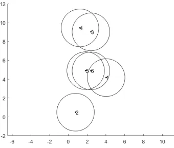
In figure 1 a plot of a small network con-sisting of six caches and eight files can be seen. Every cache has a capacity of three files. As seen in the corresponding distribution matrix (13), the files with the lowest request probabil-ity does not get stored much.

Figure 1:A small network

B=        

1 1 1 0 0 0 0 0

1 1 1 0 0 0 0 0

1 0 0 1 1 0 0 0

1 1 1 0 0 0 0 0

1 1 1 0 0 0 0 0

0 0 0 1 1 1 0 0

        (13)

In figure 2 the locations of caches of a real network in Berlin are plotted. This network consists of 62 caches, each with a capacity of three and range of 700, and 200 files. Unfor-tunately the network is too big to solve in an appropiate amount of time, so the results are run with less files, namely 40. The resulting dis-tribution matrix has dimensions 62−by−40, and the resulting probability a request is not answered is 0, 2177.

Figure 2:Berlin network

4.

A

nalysis

When solving the model every entry in the dis-tribution matrixBis a variable. So a network consisting of N caches and J files has N∗J variables. When the network is quite small the solving of the model does not take too much time, but when the network is big the runtime of the code can increase drastically. In this section there will be looked at the change of probabilities, andd also at how much the run-time increases when parameters like caches, files and range are changed.

randomness of the cache locations, to make the result more robust, every network has been ran five times and the result is their mean.

In the appendix all the figures’ correspond-ing tables can be viewed.

4.1.

Miss probabilities

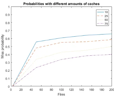
In figure 3 some networks with different amount of caches and their respective prob-abilities that a file request cannot be answered, so called ’miss probabilities’, are graphed while adding more files to the networks.It can be seen that if a network has fewer files, the probibility of missing a file is lower. This is makes sense because there are fewer files to request.

Figure 3:Miss probabilities adding files

When a network increases in the amount of caches the miss probability decreases. This is also seen in figure 4.

Figure 4:Miss probabilities adding caches

4.2.

Simple distribution

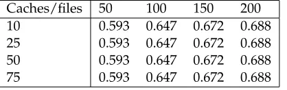
Most often existing caches save only the few most popular files. Such a simple distribution matrix consists of only 1’s the firstK(cache ca-pacity) columns and zeros in all the remaining columns. This way of distributing files is very inefficient when a lot of caches overlap. Many files will be saved in multiple caches in range of a user.

In figure 6 the change of the miss probabil-ity for a network with 10, 25, 50 and 75 caches and a cache capacity of three, are graphed while increasing the amount of files. The result is the same for each network because when only the first three most popular files are stored, no matter how many caches their are, in every area the miss probability is the same.

Figure 5:Miss probabilities adding files using a simple distribution strategy

4.3.

Runtimes

For big networks the runtime of the code will be very long. In figures 6 and 7 the increase of runtime can be seen when adding files and caches, for networks with different amount of caches.

Figure 6:Runtime increase while adding files

The more caches in a network the steeper the increase in runtime when adding files.

Figure 7:Runtime increase while adding caches

The increase of runtime when adding files to a networks seems to grow almost linear, while when adding caches to a network the runtime seems to increase exponentially.

4.4.

Cache ranges

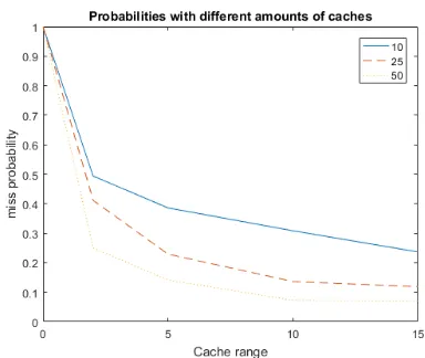
The range of caches is an important factor when distributing files over a network. When the cache ranges are large there will be many overlapping areas, causing more different files to be saved. For the graph of figure 8 networks with 10, 25 and 50 caches, all with 25 files, are tested.

Figure 8:Change of miss probabilities when cache range increases

4.5.

Variables and Constraints

When running the code ’cvx’ calculates the amount of variables and constraints in the opti-mization system. These depend on the amount of caches and files in the network, but also on the amount of overlapping areas.

For the figures in this section networks were used in which there where no overlapping ar-eas. Every cache has their own area and no caches caused overlapping areas.

This has been done because when there are overlapping areas the variables and constraints of the system change a lot. Using random networks, causing random amounts of over-lapping areas, will give many different results because of this.

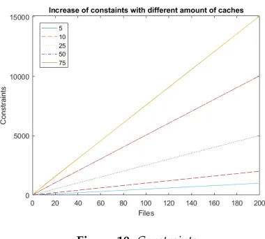
In the figures 9 and 10 the increase of vari-ables and corresponding amount of constraints, while adding more files to the networks, are graphed. Both seem to increase linear although the amount of variables increase way faster then the constraints.

Figure 9:Variables

Figure 10: Constraints

The runtimes for generating a distribution for the non overlapping networks are given in figure 11 and 12.

Figure 11:Runtimes adding files

5.

D

iscussion and

C

onclusion

By distributing files over a network of caches using the method described in this paper some internet traffic will be relieved from the current infrastructure.

Using caches efficiently does have a signifi-cant result on the amount of file requests that can be answered. The more caches, and the larger the their range, the more files can be

saved and the more file requests will be an-swered.

R

eferences

[1] Jasper Goseling Berksan Serbetci

Stochastic Operations Research University of Twente

Konstantin Avrachenkov, INRIA Sophia Antipolis

A Low-Complexity Approach to Distributed Cooperative Caching with Geographic Constraints On Optimal Geographical Caching in Heterogeneous Cellular Networks

[2] Michael Grant and Stephen Boyd

CVX: Matlab Software for Disciplined Convex Programming, version 2.1 http://cvxr.com/cvx

March 2014

[3] Negin Golrezaei, University of Southern California Andreas F. Molisch, University of Southern California

Alexandros G. Dimakis, Viterbi School of Engineering, University of Southern California Giuseppe Caire, Viterbi School of Engineering, University of Southern California

Femtocaching and Device-to-DeviceCollaboration: A New Architecture for Wireless Video Distribution 2013

[4] Nicaise Choungmo Fofack, Sara Alouf Modeling modern DNS caches2013

[5] Arpan Chattopadhyay, BartÅ ´Comiej BÅ ´Caszczyszyn

6.

appendix

Figure 13:Miss probabilities change

Caches/files 50 100 150 200

10 0.557 0.608 0.641 0.658

25 0.481 0.551 0.560 0.5862

50 0.338 0.428 0.4525

-75 0.235 0.337 0.3836

-Figure 14: Comparison to most popular distribution

Caches/files 50 100 150 200

10 0.593 0.647 0.672 0.688

25 0.593 0.647 0.672 0.688

50 0.593 0.647 0.672 0.688

75 0.593 0.647 0.672 0.688

Figure 15:Runtime change

Caches/files 20 30 40 50

5 2.406 4.431 6.037 7.795

10 9.532 12.576 18.658 23.413

15 21.802 29.945 45.954 62.950

20 45.947 55.641 79.329 102.515

Figure 16:Change of miss probabilities when cache range increases

Range/caches 10 25 50

2 0.4938 0.4114 0.2501

5 0.3858 0.2290 0.1414

10 0.3083 0.1362 0.0726

Table 1:Legenda

Symbol Description C Set of all files

J Amount of files

cj Filej

aj Probability filejis requested

N Amount of caches

K Capacity of a cache

m Cachem

Θ Set of all possible combinations of caches that can be in range of an area s Set of caches in range of an area

As The area in which all caches insare in range

ps Probability a user is in an area in range of the caches ins Acov The total area all caches cover

b(_jm) File storage index of filecjin cachem

B Storage policy matrix(NX J)

f(B) Probability a requested file is not found

Table 2:Variables

Caches/files 10 25 50 100 150 200

5 155 v 55 c 380 v 130 c 755 v 255 c 1505 v 505 c 2255 v 755 c 3005 v 1005 c

10 310 v 110 c 760 v 260 c 1510 v 510 c 3010 v 1010 c 4510 v 1510 c 6010 v 2010 c 25 775 v 275 c 1900 v 650 c 3775 v 1275 c 7525 v 2525 c 11275 v 3775 c 15025 v 5025 c 50 1550 v 550 c 3800 v 1300 c 7550 v 2550 c 15050 v 5050 c 22550 v 7550 c 30050 v 10050 c 75 2325 v 825 c 5700 v 1950 c 11325 v 3825 c 22575 v 7575 c 33825 v 11325 c 45075 v 15075

Table 3:Runtimes

Caches/files 10 25 50 100 150 200

5 0.7423 1.6297 3.1677 6.1373 9.3968 12.9194

10 1.3107 3.0522 6.0692 12.4735 19.3260 27.5507

25 3.0581 7.6029 15.7807 36.2222 57.8310 83.7663

50 6.1947 15.8061 36.0718 83.0759 140.2921 206.0263