Consumption Patterns Over Pay Periods
Clare Kelly
And
Gauthier Lanot
No 656
WARWICK ECONOMIC RESEARCH PAPERS
CONSUMPTION PATTERNS OVER PAY PERIODS
Clare Kelly
1Department of Economics,
University of Warwick,
and
Gauthier Lanot
Department of Economics,
Keele University.
November 2002
This paper establishes a theoretical framework to characterise the optimal behaviour of
individuals who receive income periodically but make consumption decisions on a more frequent
basis. The model incorporates price uncertainty and imperfect credit markets. The simulated
numerical solution to this model shows that weekly consumption functions are ordered such that
the functions within the payment period are highest in the first and the last week of the payment
cycle for all wealth levels. Using weekly expenditure data from the FES, we estimate the
coefficient of relative risk aversion (point estimates are between 1.2 and 7) and the extent of
measurement error in the data (which accounts for approximately 60% of the variance in the
data).
JEL Classification: D11; D12; D91.
Key Words: Consumption; liquidity constraints; uncertainty; credit cards
1
1. INTRODUCTION
The purpose of life-cycle models of consumption is to explain how individuals allocate
consumption optimally to different periods of their lifetime given available information about
lifetime resources, future uncertainty and the nature of financial markets (see Zeldes (1989a),
Deaton (1991), Attanasio et al. (1999), Gourinchas and Parker (2002)). The evidence shows that
attitude to risk, the rate of time preference, demographic factors and labour supply are all
important determinants of long-run consumption behaviour (see Banks et al. (2001) and
Gourinchas and Parker (2002)). The focus of the existing literature is long run consumption
behaviour over the life cycle and it is accepted that the frequency of income receipt should be
irrelevant for the pattern of expenditure within a payment period (Browning and Collado, 2001).
This paper challenges that assertion and argues further that examining such short-run behaviour
can help us to understand behaviour in the long-run.
Specifically, in this paper we consider individuals who receive a regular income (known)
on a monthly basis while their consumption decisions take place more frequently, say weekly. In
the short run income is certain, and uncertainty is assumed to arise from short run variation in
prices between weeks. Of course short run randomness in prices faced by individuals may reflect
different phenomena, like changes in the local availability of some or all goods, or variation in
the opportunity cost of some goods etc. In this paper we assume that uncertainty is gradually
“resolved” during a monthly payment period (each week) and we are interested in the optimal
consumption decision as that uncertainty is revealed2. We expect that the optimal consumption level will not only depend on the level of disposable wealth but also on the specific point in the
payment cycle at which the consumption occurs, because of this gradual resolution of
uncertainty. In such a world, along a sample path, the individual is relatively wealthier at the
time of receipt of her monthly income but faces a somewhat more uncertain future, i.e. behaviour
must take into account that there are three more weeks without payment. The last week before
payment is due, the individual is relatively poorer but uncertainty may not be so important since
the next week brings new disposable wealth. Since in general we may expect individual
preferences to exhibit some precautionary motive, consumption behaviour will respond to the
changing level of uncertainty.
In the short run the market(s) for unsecured (or even secured) borrowing of a few weeks’
duration is/are very thin. This limits the amount of borrowing possible and drives a wedge
between the return on very short-term saving and the cost of short-term borrowing on credit cards
consumption theory: how is consumption allocated across time periods when both uncertainty
and imperfect capital markets prevail. Examining optimal behaviour in this short-run framework
will inform us about behaviour under similar circumstances in the long run. Moreover, the
short-run nature of the problem allows us to abstract from the influences of demographics and labour
supply since we can argue that in the short run these characteristics are essentially fixed.
Our methodology builds on the modelling of long run consumption and follows the work
of Zeldes (1989a), Deaton (1991), and draws on the empirical methodology used in modelling
inventories and commodity prices in Deaton and Laroque (1992, 1995, 1996) and Chambers and
Bailey (1996). Our model of consumption incorporates the features of the short-run environment
i.e. periodic receipt of income, imperfect capital markets and uncertainty with respect to
consumption. We characterise the optimal solution to the model in terms of first order conditions
and then prove the existence of a unique stationary solution. For our empirical work we
parameterise the model assuming a felicity function with Constant Relative Risk Aversion.
However, since it is not possible to obtain the closed form solutions of the consumption function
with this functional form, we use numerical methods to solve the model as in Deaton (1991) and
Deaton and Laroque (1995), (for related issues see Judd (1998)). We extend beyond the current
consumption literature and use the solution of the structural model to estimate the parameters
using the Pseudo Maximum Likelihood Estimator (PMLE) of Gourieroux et al. (1984).
The UK Family Expenditure Survey (FES) is our data source. Each sampled individual
in the dataset records item level expenditure in a diary for two consecutive weeks, and provides
information on the level and frequency of receipt of regular labour income. For all individuals
who are paid monthly we determine the point in their monthly payment cycle at which they are
observed and the level of non-durable expenditure for the two observed weeks. Thus, our dataset
is a panel of two observations of expenditures in successive weeks of the payment cycle. We
exclude from our definition of non-durable expenditure any item that can be purchased but its
consumption smoothed within the home e.g. tinned food, shoes, etc…. Prima facia evidence
from the FES in Figure 1 shows the average weekly pattern of non-durable expenditure over the
payment cycle for nine different income groups. It is clear that for most groups consumption is
high in the first week when income is received, then decreases for the second and third and is
then relatively higher in the fourth week. This agrees with our intuitive argument above. It is this
pattern in weekly expenditure during a month that our structural model is designed to capture.
2
We use this data from the FES to estimate the structural model of short-run behaviour,
and find that the coefficient of relative risk aversion ranges from 1.2 to 7 for different scenarios.
This is well within the range in the literature on life-cycle models of consumption for this
parameter. Measurement error is also an important issue and we estimate that approximately
50% of the variation in the FES data is due to measurement error. Failing to take account of this
issue leads to estimates of risk aversion that are biased and makes if difficult to estimate the
model.
Section 2 of this paper presents some illustrative empirical analysis quantifying the
evidence presented in Figure 1. We provide more details on the pattern of expenditure decisions
over a payment cycle and how this pattern varies with access to credit markets, income and age.
Section 3 presents the theoretical model of consumption when income is received periodically,
incorporating a limit on borrowing and an interest rate differential between borrowing and
saving. We present the numerical solution to this model for assumed values of the parameters.
Section 4 describes the estimation procedure. The optimal consumption depends on wealth and
prices, while the data contains only expenditure observations. This is the major complication
when it comes to the estimation of the parameters of the model. Furthermore, we show that
measurement error is a significant issue in the expenditure data available and we extend the
estimation procedure to take account of this. We present Monte Carlo results on the performance
of the estimator and find that it in all cases the estimated parameters (the coefficient of relative
risk aversion and the standard deviation of the distribution of measurement error) are within two
standard deviations of the true values. We describe in a similar way the estimation procedure
that allows for the misreporting of the point in the payment cycle at which individuals are
observed. Finally, we present the estimation results. Section 5 concludes.
2. SHORT-RUN CONSUMPTION DECISIONS: EMPIRICAL EVIDENCE
To assess the importance of short run behaviour in the data we estimate a set of (quasi-)Euler
equations which allow for week specific effects, given by
[ ] [ ] [ ]
(
)
[ ]1 1 1
21 week 1 in 32 week 2 in 43 week 3 in 21 32 43 week 4 in 1
ln ln
,
it it it
it
t t t t
c α y x β
γ γ γ γ γ γ ε
+ + +
+
∆ = + +
+ + − + + +
1 1 1 1 (1)
where ∆lncit+1 : individual i’s growth in expenditure between two successive weeks,
1
it
y + : income received at the start of month (i.e. at the beginning of week 1),
1
it
x + : individual/observation specific controls (like date of survey),
[week kin t]
1,
k k
γ + : average expenditure growth between week k and k+1,,
1
it
ε + : iid stochastic mean zero error terms.
The terms γk+1,k in this equation capture the change in expenditure between two contiguous weeks in the payment period. We assume here that these changes are invariant to the calendar
time and therefore are only week specific. Hence, the sum of all changes between the second and
the first week, γ21, the third and the second, γ32, and the fourth and the third, γ43, must add up to the opposite of the change between the first and the fourth week, i.e. γ14= −
(
γ21+γ32+γ43)
. The estimation of this set of equations allows us to assess whether transition through the paymentcycle has a significant effect on consumption decisions. We also include income in order to
investigate whether liquidity constraints are important in determining short-run behaviour.
Significance of income in explaining consumption growth would indicate the importance of
liquidity constraints because the individual cannot simply borrow as necessary to achieve their
optimal consumption and so the path of consumption cannot be independent of the level of
income (see Zeldes 1989b).
Here we outline how we can extend empirical models from the existing literature (Zeldes
1989b) to deal with the problem at hand. One possible simple model to account for the
specification in (1) will make the marginal utility of consumption a function of the point in the
payment cycle at which the expenditure occurs. The point in the payment cycle acts as a shift
factor in the utility function in a similar way to the role of demographic factors in long-run
consumption models (Zeldes, 1989b, Deaton, 1992). Loosely speaking, more uncertainty can be
thought of as shifting marginal utility down, and therefore less uncertainty will shift marginal
utility up. First order conditions from dynamic models imply that marginal utility will be
smooth/constant over time and so these shift factors cause differences in the level of optimal
consumption over time. By implication consumption must be lower in the weeks with more
uncertainty. This is in effect the framework proposed by Zeldes (1989b), where he uses a
Constant Relative Risk Aversion (CRRA) felicity function in order to derive an approximation to
the Euler equation. We begin with
1
( , ) exp( ) 1
t
t t t
c
u c z z
ρ
ρ
−
=
− ,
where ρ is the coefficient of risk aversion, ct is consumption in period t and zt is the realisation
of a time specific random shift factor Zt. Our definition of consumption includes only
expenditure on non durable items e.g. perishable goods and food away from home. Hence, we
are implicitly assuming separability between non durable consumption and all other
if there is no limit on the amount of borrowing, then in each period the individual maximises the
sum of utility in all future periods in her lifetime i.e.
1 0
max exp( )
1 t t t t t c E Z ρ β ρ − ∞ = −
∑
,subject only to a budget constraint governing the evolution of wealth
(
)(
)
1 1
t t t t
w+ = +r w + −y c , t=0...∞,
where β is the discount factor,yt= yif income is received in time t andyt=0otherwise ( i.e. y is regular monthly income), and r is the interest rate. In the absence of liquidity constraints and
with perfect capital markets, the first order conditions for this problem leads to an Euler equation
which implies that discounted marginal utility should be constant on average between time
periods, i.e.
1
1 1
exp( ) (1 ) 1 exp( )
t t
t
t t
c z r
e c z ρ ρ β − + − + + + = + ,
where both r and β are assumed to be constant over time and across households. The left hand side of this equation should differ from one only by the expectation error et+1, which has mean
zero and is independent of information known at period t including monthly income. Taking a
log approximation of both sides and rearranging gives the equation for consumption growth as
( )
1{
(
1)
(
)
( )
(
1)
}
1
ln ct zt zt ln 1 r ln β ln 1 et
ρ
+ + +
∆ = − − + − + + .3 (2)
Since we can always write zt+1− =zt γt+1,t+vt+1, where γt+1,t ≡Et
[
Zt+1−Zt]
and Et[ ]
vt+1 =0, wecan express (2) as
( )
1 ˆ 1, 1ln ct+ γt+ t ηt+
∆ = + ,
where γˆt 1,t 1
{
γt 1,t ln 1(
r)
ln( )
β E(
ln 1(
et 1)
)
}
ρ
+ = + − + − + + + and
(
)
(
(
)
)
{
}
1 1 1 1
1
ln 1 ln 1
t et E et vt
η ρ
+ = + + − + + + + . Equation (1) is an empirical specification of (2),
where the parameters of the transition dummies are assumed constant over time (more precisely,
3
transition between weeks with the same position in the payment cycle have the same effect
irrespective of the calendar time period of observation).
We estimate this Euler equation using data from the FES in the UK. As described in the
introduction, the dataset allows us to create a panel of expenditure observations for two
consecutive weeks for each monthly paid individual in the survey. The FES for 1996/7, 1997/98
and 1998/99 are used but the sample is restricted to individuals who are in full time employment,
are usually paid monthly and the reported income is their usual income. The estimations exclude
“outliers” which are defined as persons whose non-durable consumption in any one week is
greater than their monthly income. These observations are less than 3% of the sample and are
distributed almost equally between credit card holders and non-holders. Their inclusion leads to
income being insignificant in each sample, but the results for the transition dummies are
qualitatively similar.
We carry out the estimation for different groups within the sample and we examine how
the significance of the payment cycle differs between these groups. Firstly, we separate the
sample into individuals who may be constrained with respect to short-term credit based on
whether they are recorded as holding a credit card in the dataset. This depends on the individual
paying an annual charge for her card and we supplement this indicator by also recording whether
the individual made any purchases on credit during her diary period. While this is not a perfect
indicator of liquidity, close to 55% of our sample is classified as unconstrained which seems
realistic although conservative. With this information we mis-classify as constrained individuals
who either did not use their credit card during the fortnight, or did not pay or recall paying an
annual charge during the previous year although they may have a card. However, following the
findings of Japelli et al. (1998), this classification may still be more accurate than a wealth to
income ratio. While the effect of uncertainty may still be significant for those with access to
credit, the importance should be reduced and so we do not expect the γk+1,k coefficients to be as large or as significant as for those without access to credit. In addition, we do not expect α, the income coefficient, to be significant for the group with access to credit since we believe they are
not constrained. We also split the sample at median income to examine whether the uncertainty
and liquidity constraints are important only for those with relatively low income. Finally, we
separate the sample based on age. Gourinchas and Parker (2002) present evidence that the buffer
stock model of accumulation of assets for precautionary reasons applies only to those below
middle age, following which accumulation of assets for retirement and bequests becomes
important. Thus we consider a sample split at age 45.
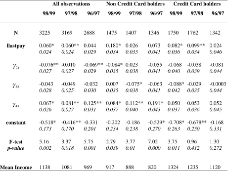
[Insert Table 1 here]
The results of the estimation of (1) are presented in Tables 1 and 2. Monthly dummies
were included to account for calendar time specific effects, although the coefficients are not
reported. We first consider the effect of the changing level of uncertainty from moving through
the payment cycle for the entire sample (Table 1). This is measured relative to the effect of
going from week four when uncertainty is least to week one when it is greatest. The importance
of uncertainty in the sample as a whole for every year is clear. γ43, the parameter that measures the transition between weeks three and four (at which point uncertainty is resolved) is positive
and significant, while we find that γ21, the coefficient which measures the transition between weeks one and two (at which point uncertainty is at its highest) is negative and significant. We
carry out F-tests where the null hypothesis is the joint insignificance of the transition dummies
and find that we reject the null hypothesis for all years of data. Income is also significant for the
pooled samples of constrained and unconstrained individuals in both 1997/8 and 1998/9 but not
in 1996/7. This indicates the possibility of liquidity constraints since consumption growth should
be independent of any information known at the time of the decision, in particular regular certain
income.
The differential effects of uncertainty are also clear when the sample is split into those
with and without a credit card (Table 1). For the constrained group, the resolution of uncertainty
remains significant while the week dummy variables are generally insignificant for the
unconstrained group. The null hypothesis of joint insignificance is clearly rejected for the non
credit card holders in all years of data. However, we also reject the null for the unconstrained
sample in 1998/9, but in line with expectations, fail to reject the null hypothesis in 1996/7 and
1997/8. The results from splitting the sample based on income and age (Table 2) indicates
clearly the importance of the changing level of uncertainty for lower income and younger
individuals. The week dummies are significant in all years for both of these groups. They are
significant in the above median income group in 1996/7, however the F-tests for all other older
and relatively wealthier groups strengthen the conclusion that their behaviour is not
systematically influenced by uncertainty.
Considering each sub sample in turn gives ambiguous results as far as the significance of
income is concerned. For example, contrary to our expectations, we find that income is
insignificant for the non credit card holders in 1996/7 and 1997/8 and that it is significant for the
credit card holders in 1997/8 and 1998/9. The misclassification of unconstrained individuals into
the constrained subsample may explain these results. Furthermore, income is generally the
of the selection.4 Splitting the sample at median income and at age 45, does not strengthen further the evidence on the presence of liquidity constraints. Indeed, income is significant for the
below median income group only in 1996/7 and is insignificant for the below age 45 group in
1997/8.
An alternative explanation for the observed pattern in expenditure could be a positive
correlation between the timing of the payment of regular bills, and other regular expenditure
some of which we define as short term consumption. If so, such a pattern should be observed in
the expenditure of all individuals, irrespective of the frequency of income receipt. In particular,
evidence of a cyclical pattern in the expenditure of weekly paid individuals would provide
evidence in favour of this explanation. Unfortunately, we cannot carry out the analysis above for
weekly paid individuals because the data does not allow us to identify when they pay regular
bills. However, a cyclical pattern in expenditure implies the same variance in the growth of
expenditure between weeks for all payment frequencies. A smaller variance of expenditure
growth for weekly paid individuals implies a smoother consumption path than the cyclical pattern
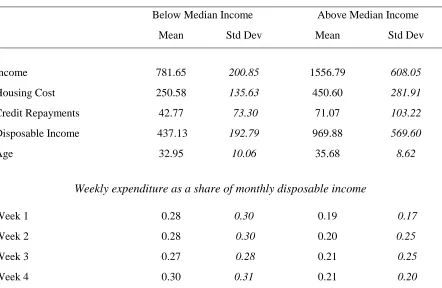
evident in expenditure of monthly paids. We show in Table 3 that the mean growth rate is
smaller in absolute terms while the standard deviation of the growth rate is larger for monthly
paid individuals. We test the null hypothesis of equality of the variances across the two groups
against the alternative that the weekly paid have a smaller variance using a conventional F-test.
The results show that the null is rejected at all levels of significance. We conclude therefore that
a cyclical pattern is more pronounced among those who are paid monthly. We interpret this
finding consistent with optimal behaviour by monthly paid individuals as they make the
transition through the payment cycle.
[Insert Table 3 here]
3. MULTI CONSUMPTION PERIODS WITHIN EACH PAYMENT PERIOD
3.1 Model of Consumption
The previous section established that the position in the payment cycle and credit
constraints are important determinants of consumption in the short-run and this section develops
a model of consumption behaviour which captures these features. There are three possible
situations for the individual: payment occurs in this period and not in the next period, payment
does not occur either in this period or next period, and payment does not occur this period but
4 In results not reported here, we correct for selectivity in credit card ownership and include the selectivity
does occur next period. Therefore a three period model is sufficient to capture the characteristics
of behaviour and simplifies the presentation of the model5. In this context, we define wealth in week one as the amount of assets (positive or negative) before income is received and, in all
other weeks as the amount of assets (positive or negative) at the start of the week after the
relevant interest rate has been applied. Here “cash in hand” refers to the sum of wealth and
income in the first week and the level of wealth in subsequent weeks. We present the optimal
consumption function as the relationship between consumption and wealth, given price. Income
enters the budget constraint only in the first week of the payment cycle and the maximum
borrowing in each time period is defined as the limit on “monthly” borrowing d , discounted by
the cost of borrowing, δ , which is incurred “weekly”. The weekly borrowing limits are given by
2 1 /(1
d ≡d + )δ , d2 ≡d/ 1
(
+δ)
, and d3≡d, and therefore the minimum wealth at the start ofeach week is given by wt+1≡ − +
(
1 δ)
dt. We also assume that the interest rate for borrowing is greater than the return on saving. The budget constraint in any time period t ist t t t t
p c ≤w + +y d , and the evolution of wealth follows the process
(
)
1 (1 ) ( )
t t t t t t
w+ = w + −y p c + +r d r−δ ,
where pt: price draw in the current period,
t
c : consumption in the current period
t
w : wealth at the start of the current period,
t
y : regular income such that yt= y if mod(3)t = 0, and yt =0 otherwise.
t
d : debt in period t, such that 0≤ ≤dt dt, r : return on savings,
δ : cost of borrowing.
We assume that yt, d , r and δ are exogenous and known with certainty and that the differential
between borrowing and saving rates is constant. Total expenditure in period t is given by p ct t.
We assume that individuals are infinitely lived, and consumption is chosen to maximise
the discounted sum of utility flows
( )
0 0
max t t
t
E β u c
∞
=
∑
,subject to the budget constraint (given above) in each period t. Standard dynamic programming
arguments suggest that we consider the value of the optimal consumption plan at time t given
5
wealth w and price p. However, the value function differs between weeks in the payment cycle
because the function reflects the proximity to receipt of income. The week 1 value function takes
account of the fact that cash on hand is at its highest in that week but that any debt will incur an
interest cost in each week until the next payment. The value function in week 3 reflects the
receipt of income in the following period, the reduction in uncertainty and the immediate
repayment of debt incurred. Thus we write a set of period specific Bellman equations, which
define the optimal consumption path as a function of wealth and price in each week, i.e. w and p.
We assume that price does not exhibit any persistence. This simplifies our analysis, in
particular expectations are not conditional on the information contained in previous price levels
and/or the history of price observed so far. The realisation of future price is denoted by π and we assume both p and π are drawn from the distribution F with support 7 over which expectations are taken. We assume that the support is closed interval p p, of \ , with +* p>0 and 1< < ∞p . The support therefore includes 1. Furthermore we assume that EF
[ ]
p =1.The week specific Bellman equations are given by(
)
{
( )
(
)
}
1 2
, subject to 0
(1
; max (1 )( ) ( ;
c d
pc w y d d d
V w p u c V r w y pc r d
δ
β δ π
2
≤ + + ≤ ≤
+ )
= + Ε 7 + + − + − ) ,
(
)
{
( )
(
)
}
2 , 3
subject to 0
(1 )
; max (1 )( ) ( ;
c d
pc w d d d
V w p u c V r w pc r d
δ
β δ π
≤ + ≤ ≤
+
= + Ε 7 + − + − ) , (3)
(
)
{
( )
(
)
}
3 , 1
subject to 0
; max (1 )( ) ( ;
c d
pc w d d d
V w p u c β V r w pc r δ d π
≤ + ≤ ≤
= + Ε 7 + − + − ) ,
where the felicity function ( )u c is assumed to be increasing, monotonic and concave. We assume
that the discount factor β is such that β(1+δ) <1 i.e. the consumer is “impatient” and has a
preference for consumption in the present. For a given wealth and price realisation, the control
variable consumption is chosen to maximise the right hand side, subject to a lower limit on
negative wealth. The problem fulfils the conditions for continuity and differentiability of the
value function as given by Benveniste and Scheinkman (1979). Indexing each specific week in
the payment cycle by k, the set of Lagrangian equations which define the constrained maximum
are given by
(
) ( )
(
)
(
)
( )
(
)
1 2 1
1 2
, ; , , (1 )( ) ( );
( ) ,
k k k
k k k
L c d u c E V r w y pc d r
pc w y d d d d
γ µ µ β δ π
ψ µ µ
+
= + + + − + −
− − + + + + −
7
for k = 1,2,3 and where k+1 = 1 if k=3. This gives rise to the first order conditions (where *
denotes the optimal consumption level)
(
) ( )
( )
(
)
( )
(
)
(
)
(
)
* *1 2 * 1 *
* *
1 2 1 *
1 2
* *
1 2 * *
* *
1 2 *
1 * *
1 2 *
2
, ; , ,
' (1 ) . 0,
, ; , ,
( ) . 0,
, ; , ,
( ) 0,
, ; , ,
0,
, ; , ,
0.
k k k k k
k
k k k k k
k k k
k k k k
k
k k k
k
k k k k
k
L c d EV
u c r p p
c w
L c d EV
r
d w
L c d
pc w y d
L c d
d
L c d
d d
γ µ µ
β ψ
γ µ µ
β δ ψ µ µ
γ µ µ ψ
γ µ µ µ
γ µ µ µ + + ∂ ∂ = − + − = ∂ ∂ ∂ ∂ = − + + − = ∂ ∂ ∂ = − − + ≤ ∂ ∂ = ≥ ∂ ∂ = − ≥ ∂ (4)
The solution to this problem can be characterised by examining different values of the
multipliers. Only four combinations of the multipliers are possible. We now describe each
possible “regime” of the solution. In what follows λ(c) denote the marginal utility of consumption.
Regime 1: pc*< +w yk, *d = 0, ψk=0,µk1>0,µk2=0,
( )
( )
* 1 *
1
(1 )E k k c c r p λ λ β π + = + .
In this regime the agent does not consume all cash in hand. Hence borrowing is zero, µk1>0,
2
k
µ =0, and the positive wealth carried over to the next period earns return r. The Euler equation for this regime (the final equality above) implies that the capital market imperfections do not
constrain behaviour. The real marginal utility of current optimal consumption is given by the
value of marginal utility of optimal consumption in the next period, discounted at β +
(
1 r)
. It is never optimal to borrow and not consume that extra cash when the cost ofborrowing is greater than the return on savings. This rules out regimes where ψk= 0, µk1=µk2= 0, and ψk = 0, µ >k1 0, µ =k2 0. In all other cases ψk>0, i.e. consumption is greater than or equal to cash in hand and assets are run down or at least not accumulated.
Regime 2:pc*= +w yk, *d = 0, ψk>0, µk1>0, µk2= 0,
( )
*1 1 k
k
w y
c
pλ pλ p
+
=
.
marginal utility is simply the marginal utility of available cash in hand. No assets are carried
over to the next period.
Regime 3:pc*= +w yk +d*, 0<d*<d , ψk >0, µk1=µk2=0,
( )
( )
* 1 * 1 k k c c p λ
λ β δ
π
+
= (1+ )Ε
.
In this third regime, the level of debt d is positive but below the limit, * ψk>0 and µk1 =µk2=0, and consumption is equal to the sum of cash in hand and d . Negative wealth of * − +
(
1 δ)
d* is carried into the next period. The Euler equation is fulfilled in an unconstrained way becauseoptimal borrowing is below the limit. The real marginal utility of optimal consumption in the
current period is equal to the value of optimal consumption in the next period discounted at
(
1)
β +δ .Regime 4: pc= +w yk +dk, *d =d, ψk>0,µk1 =0, µk2>0, 1
( )
* 1 k k kw y d
c
pλ pλ p
+ +
=
.
In this last regime the individual borrows up to her limit, ψk>0, µk2>0 andµk1=0. Even at the maximum level of borrowing, consumption is still below that which would be chosen if the
borrowing limit did not exist. In this case, the solution is to consume the maximum amount
possible (cash in hand plus maximum borrowing d ), and carry maximum debt k − +
(
1 δ)
dk into the next period. The Euler equation implies the solution for current marginal utility is equal tothe marginal utility of the sum of all available cash in hand and maximum borrowing.
The optimality conditions for these four regimes can be summarised in an augmented
Euler equation that relates consumption decisions in any two periods, k and k+1
( )
( )
( )
* 1 * 1 *(1 )E ,
1 1
max min , ,
1 k k k k k k c r c w y c
p p p
w y d
p p
λ β
π
λ
λ λ β δ
π λ + + + +
= (1+ )Ε
+ +
, (5)
The minimum in this expression arises because capital market imperfections prevent an
individual from receiving a return equal to δ on saving. If this is optimal but saving at r is not, the individual will not save and so will have a higher level of consumption (and therefore a lower
marginal utility) than if saving at δ were possible. The minimum condition captures this limitation on behaviour. Hence this expression is a generalisation of the first order conditions in
We follow Deaton and Laroque (1992, 1996) and assume that a stationary solution to (5)
exists. This solution defines the optimal relationship between expenditure, wealth and prices,
and so the consumption function in each week of the payment cycle, k, described by nominal
value of wealth and prices, is given by *
(
)
; /
k k
c =g w p p.
We assume gk
(
w p;)
0,w ∂ > ∂ and
(
;)
0 kg w p
p
∂
<
∂ . The marginal utility of money/wealth
[ ]
; kq w p is given by the real value of marginal utility of optimal consumption
( )
* /k
c p
λ and
therefore q w p =k
[ ]
; 1 1 gk(
w p;)
pλ p
. Writing the Euler equation (5) in terms of the marginal
utility of money, gives the following set of functional equations to which there are unique
solutions q w p given by k
[ ]
;[ ]
[ ]
(
)
[ ]
(
)
1 1 ;(1 ) (1 )( ; ; ( ),
1
max min , (1 )( ; ; ( ) ,
1 k
k k k
k
k k k
k k
q w p
r q r w y p pq w p dF
w y
q w y p pq w p dF
p p
w y d
p p
β λ π π
λ β δ δ λ π π
λ −1 + −1 + = + + + − +
(1+ ) + + −
+ +
∫
∫
7 7For ease of notation define the functions
[ ]
(
)
(
[ ]
)
1 k ; , , (1 ) k 1 (1 )( k k ; ; ( )
H q w p w p =β +r
∫
7q + +r w+y −pλ−1 pq w p πdF π ,1 w yk
p p
λ= λ + ,
[ ]
(
)
(
[ ]
)
2 k ; , , (1 ) k 1 (1 )( k k ; , ( )
H q w p w p =β +δ
∫
7q+ +δ w+y −pλ−1 pq w p πdF π ,1 w yk dk
p p
λ= λ + +
,
where H q w p w p and 1
(
k[ ]
; , ,)
H2(
q w p w p are the expected discounted marginal utilities k[ ]
; , ,)
of saving, respectively, borrowing, for current wealth and price, w, p, and marginal utility ofmoney q w p in week k. Following the arguments in Deaton and Laroque (1992) and in k
[ ]
; Bailey and Chambers (1996), we show the following theoremTheorem 1. There is a unique set of functions q w p , the stationary solutions to the k
[ ]
,functional equations (6) above, which are continuous in wealth and price and non-increasing in
wealth. In addition the solutions can be characterised as follows
[ ]
; kq w p =H q1
(
k+1[ ]
w p w p; , ,)
, when β(1+r)∫
7qk+1[ ]
0;π dF( )π ≥λ;[ ]
; kq w p =λ, when
[ ]
[ ]
1 1
(1 ) 0; ( ) , and
(1 ) 0; ( ) ; k
k
r q dF
q dF
β π π λ
β δ π π λ
+ + + ≤ + ≥
∫
∫
7 7[ ]
; kq w p =H2
(
qk+1[ ]
w p w p; , ,)
, when[ ]
1 1
(1 ) (1 ; ( ) , and
(1 ) 0; ( ) ;
k k
k
q d dF
q dF
β δ δ π π λ
β δ π π λ
+ + + − + ) ≥ + ≤
∫
∫
7 7[ ]
; kq w p =λ whenβ(1+δ)
∫
qk+1− + )(1 δ dk;πdF( )π ≤λ7 .
Proof: Available upon request.
The theorem sets out the conditions for each regime: positive saving is optimal when the
wealth level is sufficiently high so that the real marginal utility from consuming all cash on hand,
λ, is below the discounted value of the marginal utility of money from zero savings. In this case, consumption is substituted towards the future so that current marginal utility increases and
future marginal utility of money decreases until the unique level of saving that results in equality
between the two terms is reached. When the wealth level is such that the real marginal utility
from consuming cash in hand is above the discounted marginal utility of zero savings, the
individual has an incentive to increase consumption and carry negative wealth into the next week.
However, the cost of borrowing δ may bring the discounted future marginal utility of zero borrowing above the marginal utility of cash in hand, in which case the preference for higher
consumption is not strong enough for the individual to borrow at δ. In this case, neither borrowing nor saving occurs. If the wealth level is sufficiently low, it is optimal for the
individual to have a positive level of borrowing (below the limit) which decreases current
marginal utility of consumption while increasing the future marginal utility of wealth.
Borrowing remains below the limit while the marginal utility from maximum negative wealth in
the next period is above the marginal utility of maximum possible consumption today. If
however, the individual would choose a level of consumption so high relative to the real value of
wealth that borrowing greater than the maximum possible would be optimal, then at maximum
debt d the individual would further decrease current marginal utility of consumption by
borrowing and increasing consumption, and so the optimal outcome is to borrow the maximum
3.2 Numerical Solution to the model
The functional equation (6) is analytically intractable and so we solve the model using the
standard numerical methods of dynamic programming (see Deaton (1991, 1992) for a clear
exposition and Judd, (1998)). The calculations are simplified because the optimal consumption
function is homogenous of degree 1 in y (See Imrohoroglu, (1989), and Gourinchas and Parker,
(2002)). This allows us to calculate the relationship between consumption as a proportion of y
and wealth as a proportion of y. This reduces significantly the computation burden. We set the
upper bound on wealth to a multiple of income, while the lower bound is defined by the credit
limit. We discretise the wealth space into W grid points where ω =1,.,.,.,W, and the price
distribution with M grid points where m=1,.,.,.M so that the solution is calculated at each point in
the W × M matrix of grid points. Linear interpolation (or non linear methods like splines)
allows us to calculate the optimal consumption for any combination of wealth and price within
the grid. In calculating the solution, we assume CRRA preferences with felicity function of the
form
( )
1 11
u c c ρ
ρ
−
=
− for
ρ > 1
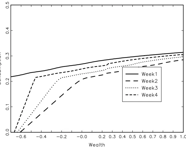
where ρ is the coefficient of relative risk aversion. This numerical solution is shown in Figure 2 where we assume β = 0.985, and ρ = 2.5, values generally accepted in the literature for these parameters. We exaggerate the cost of borrowing in this case so that the regimes of the solution
are clearly evident. Consumption and wealth are shown as proportions of income. We assume
that the limit on borrowing is set at two-thirds of income and that prices are distributed uniformly
with mean of 1 and support from 0.75 to 1.25. The solution is shown for the same price draw in
each week. We show the solution for four weeks within each payment cycle which most closely
resembles the short-run problem faced by individuals who are paid monthly and consume weekly.
[Insert Figure 2 here]
This solution means that for any given wealth level and draw of price, we can calculate
the consumption behaviour of the individual in any week. The liquidity constraint only binds in
week four so that even when there is already some borrowing in week two or three, the remainder
is never exhausted in those weeks because of the infinite cost of zero consumption. Hence, the
fourth regime is evident only in week four. The other regimes, and the kinks at which the
solutions switch between these regimes, are evident in all weeks. For all levels of wealth,
consumption is highest in the week when income is received, lowest in the next week and the
increasing over the remaining weeks. However, this ranking of the weekly consumption
functions is not unique to the CRRA utility function: the same pattern holds for other utility
functions within the class of HARA functions because these preferences imply precautionary
quarter of income is always attainable in the first week of the payment cycle even when debt is at
its maximum. This is a critical feature of the model and it has important implications when we
fit the model to the data.
4. ESTIMATION OF MODEL
The previous section described a model of short-run consumption which incorporates the
characteristics of the environment faced by many individuals: periodic receipt of income, a
differential between the cost of borrowing and the return on saving, and an upper bound on the
amount of borrowing possible. Income is certain and uncertainty arises because the price of
weekly consumption is random. In this section we show how the model can be estimated with
repeated expenditure data alone and how we can extend the estimation procedures to take
account of some measurement error in the data. We carry out a Monte Carlo study of the
performance of the estimator both before and after we include measurement error in the
parameter vector. We then describe the data and the results of the estimation on a subsample of
the FES in the UK.
4.1 Estimation without Measurement Error
The simulated policy function shown in Figure 2 allows us to relate any level of wealth and price
to the optimal consumption by linear interpolation between grid points. In what follows we drop
the index for the week (k) and assume that for each individual observation the index t is
informative about both calendar time and position in the individual payment cycle. Therefore the
weekly consumption function, g w pt
(
; ,θ)
, is a function of wealth and price given the vector of parameters θ, and implicitly depends on the individual’s position in the payment cycle. If wealth and price were observed, estimating the model from the data available would then berelatively straightforward. However, neither of these variables is observed. Instead, we exploit
the fact that we observe two successive weekly expenditures for each individual. We use the
policy functions to give the relationship between expenditure observations in adjacent time
periods rather than between wealth and prices in the same time period. We achieve this by taking
expenditure in week t and inverting the policy function for that week for a given price. That
gives the level of wealth consistent with the expenditure observation, i.e. observed expenditure
gives an implied level of wealth
(
)
1
; ,
t t t t t
w =g− p c p θ .
The success of this strategy relies upon the monotonicity of the function to give a unique
t
w is calculated, the cash on hand carried into the next period t+1 can be calculated using the
equation for the evolution of wealth
(
)
1
1 (1 )( ; , )
t t t t t t t t
w+ = +ζ g− p c p θ + −y p c ,
where y=y if income is received in period t, and y=0 otherwise, ζ δ= if (wt− p ct t)< 0, and
r
ζ = otherwise. Conditional on expenditure in t and price outcomes in t and t+1, (pt, pt+1
respectively), expenditure in t+1 can therefore be calculated as
(
)
(
(
)
)
(
1)
1 1 1 1 ; , ; 1,
t t t t t t t t t t
p c+ + =g+ +ζ g− p c p θ + −y p c p+ θ .
Taking the expectation over the price distribution in the second period, we can obtain the
expectation of expenditure for week t+1 conditional upon the observed level of expenditure in
the week t, the price outcome in the week t, and the parameter vector θ. This expectation is given by
[
]
(
(
)
(
(
)
)
)
1 1
1
1 1| , , 1 1 ; , ; 1, | , , .
t t
p t t t t t p t t t t t t t t t t t
E + p c+ + p c p θ =E + g+ +ζ g− p c p θ + −y p c p+ θ p c p θ
However the implied level of cash on hand wt =gt−1
(
p c pt t; t,θ)
must be calculated for all possible first period pricesp . Therefore taking an expectation again over the price distribution tin the first period gives the conditional expectation of expenditure in t+1 given expenditure in t
as
(
)
[
]
(
)
(
(
)
)
(
)
1 11 1 1 1
1
1 1
; | , , | ,
1 ; , ; , | , , | , .
t t
t t
t t p p t t t t t t t
p p t t t t t t t t t t t t t
e p c E E p c p c p p c
E E g g p c p y p c p p c p p c
θ θ θ
ζ θ θ θ θ
+ + + + + + − + + = = + + −
Applying the Law of Iterated Expectations to the calculation of a variance, we obtain the
conditional variance of expenditure in t+1 given expenditure in t as,
(
)
(
(
)
)
[
]
(
)
[
] (
)
(
)
1 1 1 21 1 1 1 1 1
2
1 1 1 1
2
1 1 1 1
; ; | , , | , | , , | , , | , | , , ; | , . t t t t t t
t t p p t t t t t t t t t
p p t t p t t t t t t t t t t
p p t t t t t t t t t
v p c E E p c e p c p c p p c
E E p c E p c p c p p c p p c
E E p c p c p e p c p c
τ
θ θ θ θ
θ θ θ
θ θ θ
+ +1 + + + + + + + + + + + + + + + + = − = − + −
The first term arises from the uncertainty of prices in the second period and is the
variance of each possible future value of expenditure p ct+1 t+1 around each conditional
expectation of future expenditure
[
]
1 1 1| , ,
t
p t t t t t
E + p c+ + p c p θ . The expectation of this variance is
expectation of future expenditure
[
]
1 1 1| , ,
t
p t t t t t
E + p c+ + p c p θ (given current price p ), around the t
expectation unconditional on price,
[
]
1 1 1| , , | ,
t t
p p t t t t t t t
E E + p c+ + p c p θ p c θ. This term arises
because current price is not observed by the econometrician and so the conditional expectation of
future expenditure must be calculated over all possible prices today. Deaton and Laroque (1995)
refer to these terms as the within and between variance respectively. The within variance
captures the variance of future expenditure conditional on each current price draw and is
common to the individual and the econometrician. The between variance captures the variance
across possible current price draws and exists only for the econometrician because current price
is not observed. The model is estimated using the Pseudo Maximum Likelihood Estimator
(PMLE) of Gourieroux et al., (1984). Following Deaton and Laroque (1995, 1996), we use a
second order PMLE i.e. we use the first two moments of the conditional distribution of the
expenditure in t+1 given expenditure in t, and use the p.d.f. of the normal distribution to
calculate the pseudo likelihood function. The non-differentiability of the policy function at the
points where the solution switches between the four regimes carries through to the conditional
moments of the distribution of expenditure. Therefore the pseudo likelihood function will also
be non-differentiable with respect to the parameters at these points. However, Laroque and
Salanié (1994) show that PMLE gives consistent estimates of the parameters despite this
non-differentiability and also show that a second order PMLE is almost as efficient in finite samples
as Full Information Maximum Likelihood, when estimating parameters from “badly-behaved”
likelihood functions arising from non-differentiable models. Michaelides and Ng (2000) in
addition prove the superiority of PMLE over simulation methods in estimating parameters in
models where the likelihood is non-differentiable.
The mean of the pseudo log-likelihood function can be written as
( )
(
(
(
)
)
)
(
(
)
)
2
1 1 1 1
1 1
1 1 1 1 1
;
1 1 1
ln ln ln ;
;
N N N
jt jt jt jt
j jt jt
j j jt jt j
p c e p c
L l v p c
N N v p c N
θ θ θ θ + + + + + + = = + + = −
=
∑
= −∑
−∑
. (7)The asymptotic variance covariance matrix of N
(
θ θ− 0)
for the PMLE is calculated as(
)
1 1
'
V =J− G G J− , (8)
where G is a N×rows(θ) matrix with generic element ji ln j
i l G θ ∂ =
∂ and J is a rows(θ)×rows(θ)
matrix with generic element
2 ln ih i h L J θ θ ∂ = ∂ ∂ .
Throughout the analysis we assume that the price distribution is the same in all periods
values from 7 , the support of F. The expectations are therefore calculated simply as weighted averages of the outcome for each price draw where the weights are the probability of each price
outcome in both periods, denoted by pr(pm) and pr(ph)
(
)
[
]
( )
( )
(
(
)
(
(
)
)
)
1
1 1 1 1
1 1
1 1
,
pr ; , ; , ,
; | , | ,
pr 1
t t
p
m h
t t p t t t t t t
M M
t t t t m t t h
h m
t
e p p
p g p
p c E E c p c p c
p g p c p p c
θ θ θ
ζ θ θ
+ + + + + − + = = =
=
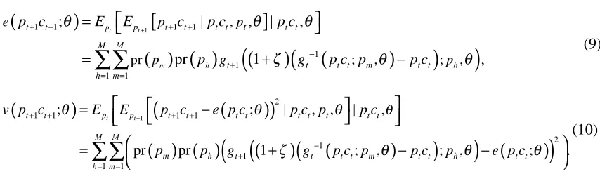
∑∑
+ − (9)(
)
(
(
)
)
( ) ( )
(
(
(
)
(
(
)
)
)
(
)
)
1
2
1 1 1 1
2 1 1 1 1 , ; ; | , , |
pr pr 1 ; , ; , ; .
t t
t t p p t t t t t t t t t
M M
m h t t t t m t t h t t
h m
v p c E E p c e p c p c p p c
p p g g p c p p c p e p c
θ
θ θ θ
ζ θ θ θ
+ + + + + − + = = = − =
∑∑
+ − − (10)These are calculated for each observation and are then substituted into the pseudo likelihood
function in (7) which is then maximised with respect to θ.
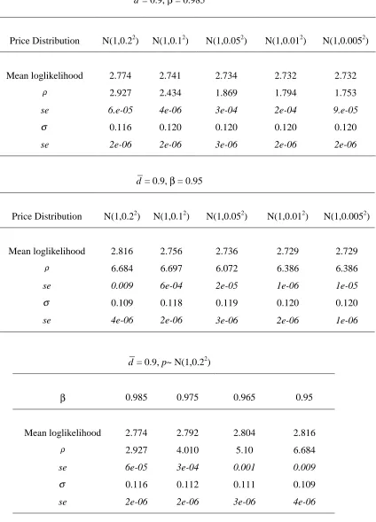
Monte Carlo Study
We carry out a Monte Carlo study to investigate the small sample properties of the PMLE in this
framework using β = 0.95, δ = 0.4% and r = 0. The parameter vector in the estimation procedure could include β ρ δ, , ,r d, and possibly the parameters of the price distribution. However we do not try to identify all those parameters from the data and instead restrict the
estimation to the coefficient of risk aversionρ. The replications are carried out for three values ofρ (1.5, 2.5, 5), and for two different price distributions (normal and uniform). In the case of the uniform distribution, prices can take on any of six equally spaced discrete values between
0.75 and 1.25, for which the expectation is one. We use a normal distribution N(1,0.172) so that it has the same support as the uniform distribution but twice the variance. This is discretised by
six points, each point being the mid-points of the interval within which 1/6 of the density lies.
(See Deaton and Laroque, 1996). For each of these set-ups we draw 100 datasets of either 500 or
1000 observations. When estimating just one parameter, we use a simple golden-section
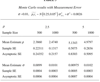
[image:21.595.85.512.118.242.2]procedure to find the maximum and find this very fast and reliable. The results are presented in
Table 4. The empirical distribution of the estimator is very close to the asymptotic variance
given by (8) and in all cases the estimated parameter is within two standard deviations of the true
value. All the maxima are robust to changing the starting values and the results suggest that there
are no obvious problems within the estimation procedure.
[Insert Table 4]
4.2 Estimation with Measurement Error
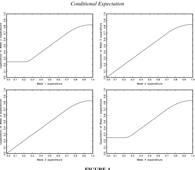
Figure 3 shows the conditional expectation in (9) and it is obvious that over a large part
of the expenditure values the conditional expectation is close to a 45o line in all weeks. Therefore we do not expect to see very large changes in expenditure between adjacent weeks.
However this is not what we find in the data. Figure 4(a) shows the kernel estimates of the
density of the proportional change in expenditures between weeks two and three from a
simulated dataset where prices are drawn according to the distribution N(1,0.22), 0.95β = ,
ρ = 2.5, d =0.66. Figure 4(b) shows the same for the dataset from the FES. The mean change between expenditure in weeks 2 and 3 in the simulated data is –1.5% with a standard deviation of
22%, while in the FES data the mean is –13% and the standard deviation is 90%. Clearly the
variation between weeks in the FES is enormous relative to the simulated data. Even if we
double the variance in the price distribution from 0.04 to 0.08, the standard deviation in the
simulated data only increases to 35%. It does not seem reasonable that these differences arise
from greater variance in prices faced by actual individuals than we allow for in the simulation (a
variance of 0.08 implies the standard deviation of the price distribution is 0.28 which seems
unrealistic).
In addition, a simple linear regression of expenditure in t+1 on t gives a coefficient close
to 0.75 in the simulated dataset while in the actual data the coefficient is closer to 0.35. This is
symptomatic of the attenuation bias resulting from measurement error. We now describe how we
extend the estimation procedure to account for the presence of classical measurement error.
[Insert Figure 4 here]
If classical measurement error exists in the data, then the observed expenditure is the sum of true
expenditure p c plus noise t t* εt, i.e. kp ct t = p ct t*+εt. The conditional expectation of interest is now
k
(
)
k k k1
1 1
;
t t 1 1| , , | ,t t p p t t t t t t t
e p c+ +
θ
=
E
E
+ p c+ + p c p θ p c θand the variance becomes
k
(
)
(
k(
k)
)
k k1
2
1 1; t t 1 1 ; | , , | ,
t t p p t t t t t t t t t
v p c+ + θ =E E + p c+ + −e p c θ p c p θ p c θ
.
In this case, it is the expectation and variance of noisy expenditure in t+1 that are used in the
PMLE in (7) and these moments are conditional on the observation of the noisy expenditure in t.
However, the methodology outlined in the previous section to estimate the parameters of the
model in Section 3 is based on the relationship between true expenditure data in adjacent time
periods. Therefore we need a way to recover the true expenditure observation from the