Nonlinear controllability via the initial state : with application to the spread of rabies

A Thesis Submitted for the Degree of PhD at the University of Warwick

http://go.warwick.ac.uk/wrap/73383

This thesis is made available online and is protected by original copyright. Please scroll down to view the document itself.

Application to the Spread of Rabies

Neil D Evans

Thesis submitted for the degree of Doctor of Philosophy

to the University of Warwick

Mathematics Institute

University of Warwick

Coventry CV 4 7 AL

of this thesis.

Acknowledgements VI

Declaration VI

Summary V1l1

Introduction 1

1 The Control Problem 9

1.1 Rabies and its control . . 9

1.1.1 What is rabies? 10

1.1.2 A history of rabies in Europe . 11

1.1.3 Control methods for rabies 11

1.1.4 The control problem

....

13

1.2 A mathematical model for controlling the spread of rabies 14

1.2.1 The basic model

...

15

1.2.2 The extended model 18

1.3 Analysis of extended model. . 21

1.3.1 Analysis of steady states 21

1.3.2 Some remarks. . . 27

1.3.3 Time dependence of vaccination procedures . 28

1.4 Mathematical formulation of the control problem 30

2 Controllability via the Initial State

₃₂

2.1.1 The abstract Cauchy problem . 2.1.2 Unboundedness of nonlinearity 2.2 Existence of a mild solution ..

2.2.1 The fixed point problem

2.2.2 Unboundedness of nonlinearity . 2.2.3 Application of a fixed point theorem . 2.3 Computing control by iteration .

2.3.1 Existence of solutions .

2.3.2 Convergence ofiterative scheme . . 2.4 Choosing the target output . . . .

2.4.1 Some preliminary results . 2.4.2 Minimising the actual output .

3 Perturbed Systems 3.1 The perturbation.

3.1.1 Associated mild evolution operator 3.1.2 Extension of the mild evolution operator. 3.2 Mild form for perturbed systems . . . . .

3.2.1 System equation is well-defined 3.2.2 Existence of mild solution 3.3 A semilinear system . . . .

3.3.1 Existence of a mild solution 3.3.2 Existence of a classical solution

4 General Example 4.1 The basic model .

4.1.1 The spaces 4.1.2 The operators .

4.2 Model considered as a perturbed system

36 40 41 42 49 50 53 54 58 60 61 64

69

70 71 79 81 82 87 91 92

. . .

.

.

96

106

· 107

...

· 107

4.2.1 Assumptions for evolution operator _{· 123}

4.2.2 Assumptions for mild form. . _{· 128}

4.3 A semi linear general example _{· 142}

4.3.1 A mild solution exists · 142

4.3.2 A classical solution exists · 144

5

Controlling the Spread of Rabies

147

5.1 Rabies model as a semilinear system . _{· 148}

5.1.1 Model formulation . . · 149

5.1.2 Existence of a solution · 156

5.2 Applying general theory to rabies model . · 160

5.2.1 Model formulation . . . · 161

5.2.2 Rabies model as a perturbed system · 162

5.2.3 Solving the control problem · 167

5.3 Numerical results . . . · 172

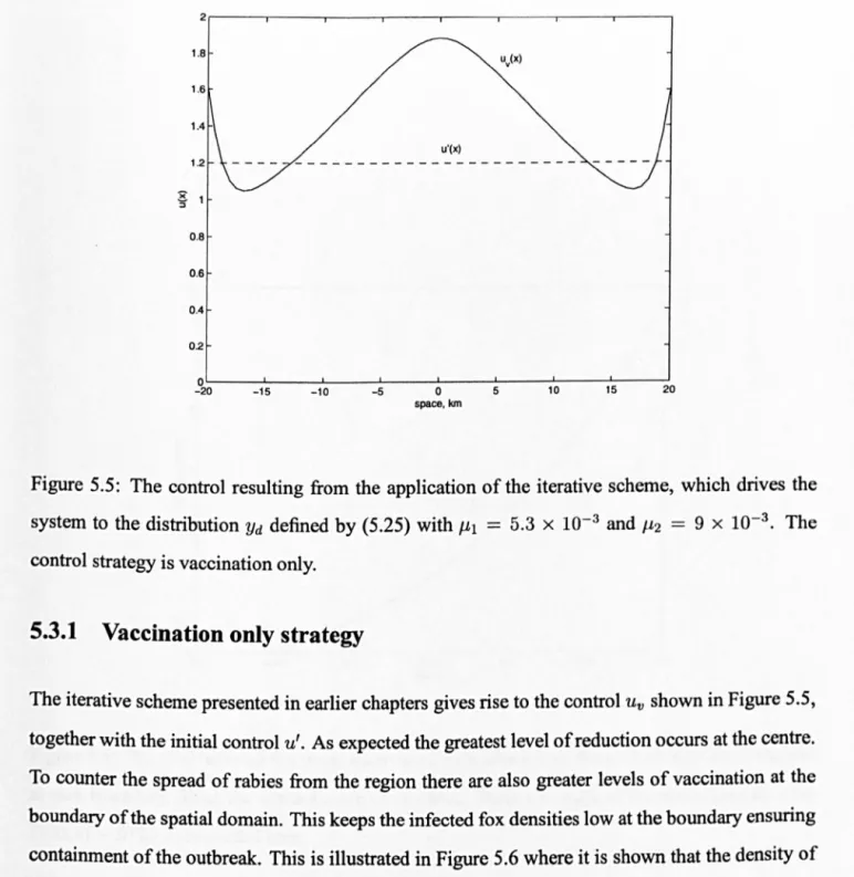
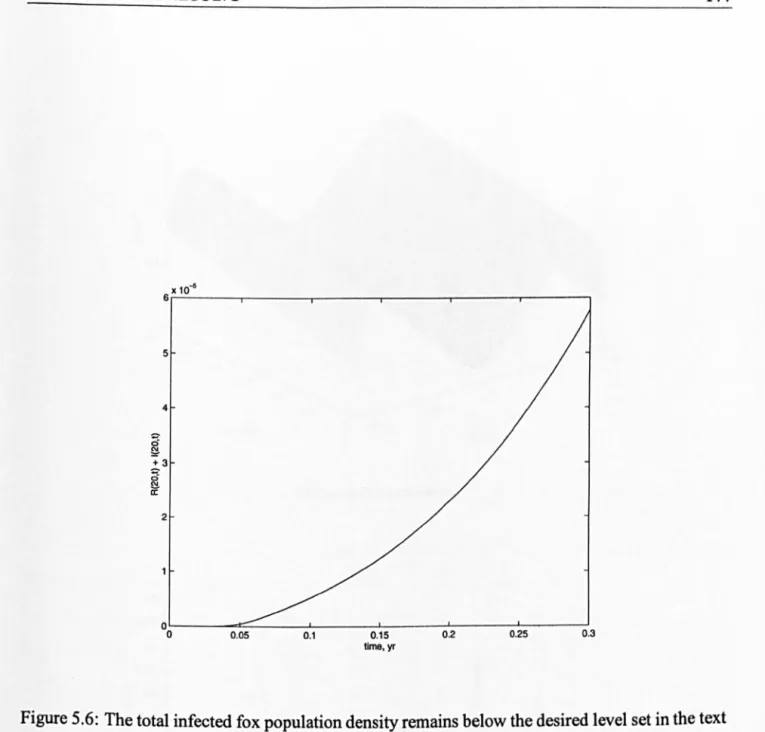
5.3.1 Vaccination only strategy . · 176

5.3.2 Culling only strategy . . . · 179

5.3.3 Combined vaccination and culling strategy · 184

A Useful Results

187

B Source Code for Numerical Simulations

189

Bibliography

207

2.1 Geometric interpretation of minimisation problem .

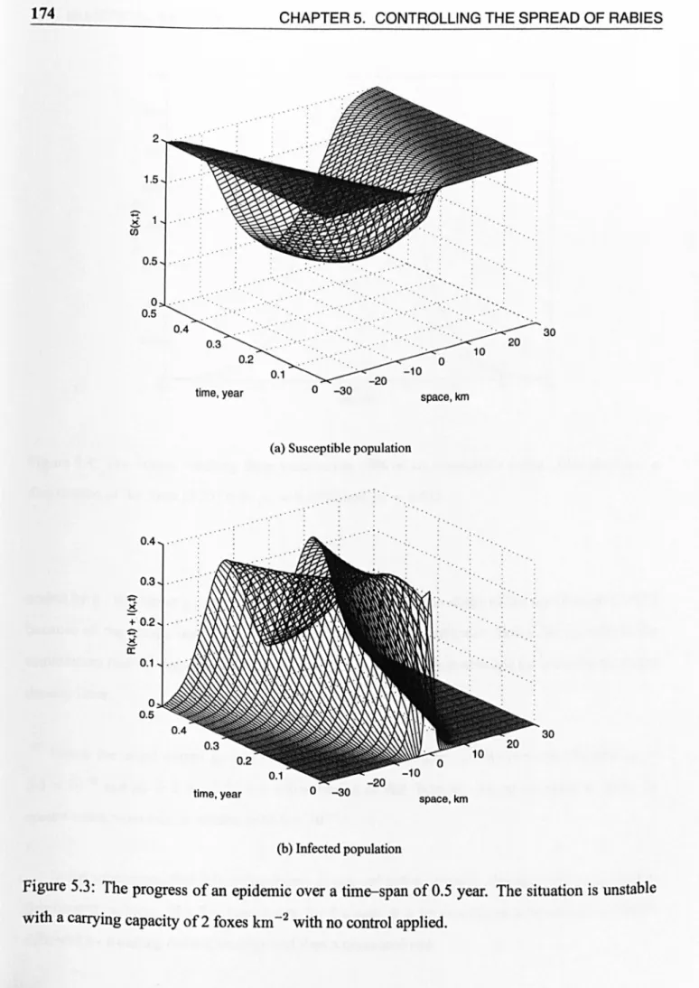
5.1 Checking TV VI for the rabies model. 5.2 Initial distribution of rabid foxes . . . . 5.3 The progress of an epidemic . . . . 5.4 The output resulting from the initial guess .. .

5.5 The control returned by the iterative scheme (vaccination). . 5.6 Infected population density at the boundary (vaccination). . . . 5.7 The effect of the control (vaccination) . . . . 5.8 Closer look at the evolution of the rabid population density ..

5.9 Comparison between actual output and target (vaccination) . . . . 5.10 The control returned by the iterative scheme (cull). .

5.11 The effect of the control (cull) . . . . 5.12 Infected population density at the boundary (cull). . . 5.13 The control returned by the iterative scheme (combined). 5.14 The effect of the control (combined) . . . . 5.15 Infected population density at the boundary (combined).

. . 65

1.1 Values for the model parameters . . . . 1.2 Recovery of susceptible population density (K = 2) . 1.3 Recovery of susceptible population density (K = 4.6) .

Acknowledgements

17 29 29

I wish to express my deep gratitude to Prof. Tony Pritchard who has been a source of guidance and encouragement to throughout this work. The work in this thesis was funded by an EPSRC studentship and so a big thank you to them.

Thank you to my colleagues in the School of Engineering who have had to put up with their Research Assistant spending a lot of his time writing this thesis. I would particularly like to thank Prof. Keith Godfrey for giving me so much time off and Dr. Mike Chappell for some helpful discussions.

Thanks also to Stephen Williams who wrote the Makefile used to compile my computer pro-grams and for providing help for all of my programming questions.

Finally, thanks to God, lowe everything to Him.

Declaration

Journal of Mathematics Applied in Medicine and Biology subject to corrections:

The Summary is an expanded fonn of the abstract. Chapter 1 provides additional background infonnation from the ecology and biology literature and includes an analysis of the steady states of the extended model. Other material from Chapter 1 is based on that in the paper.

The paper summarises the use of the fixed-point theorem to solve the control problem when the nonlinearity maps the state-space into itself. Furthermore, the time-varying perturbation P(·)

is assumed to be bounded.

Summary

There are many problems in medicine and biology involving some kind of spatial spread. Often the aim in such problems is to control the spread. A large proportion of medical and biological systems distinguish themselves from the types of system found in engineering by the way the control acts. This is illustrated by considering the specific example of the spread of rabies among foxes

A brief description of a model for the spatial spread of rabies among foxes, developed by Murray et al. (1986), is given. This model is then extended to include the control mechanism. The problem is to prevent the spread of the rabies virus by vaccinating or culling foxes via the distribution of bait in a region around an observed outbreak.

The extended model can be formulated as a nonlinear time-varying control system described by partial differential equations. In contrast to most engineering type control problems the control does not continuously affect the system but only acts through the initial distributions. A general theory is developed for dealing with such nonlinear systems by the use of a fixed point theorem.

In a similar way to Pritchard and Salamon (1987) and Hinrichsen and Pritchard (1994) the dynamics are considered on a triple of Banach spaces Z C Z

c

Z to allow for the possible unboundedness of the nonlinearity. Thus the nonlinearity is considered as a map from Z into Z.

A mild form of the time-varying system is introduced to allow for a wider class of nonlinearities. Assumptions are introduced so that the mild form of system equation is well-defined and has a fixed point that, at least partially, solves the control problem.

An adaptive scheme is introduced that constructs the control that gives rise to the fixed-point but is easier to implement computationally. This scheme is less intuitive than that provided by the fixed point theorem. However the method exploits the existence of the fixed point while only requiring the final states (and not the states on the whole time interval) to be stored at each step.

By assuming that the linear part of the system is a time-varying perturbation of a time-invariant operator it is shown how a mild form for the system equation can be derived from the original dynamics. Moreover suppose that the time-invariant operator is the generator of a strongly contin-uous semigroup. Then the conditions for the mild form of the system to be well-defined and have a fixed point can be reduced to conditions on the semi group and perturbation.

Existence theorems are provided for solutions of semilinear systems with unbounded nonlin-earities.

This thesis is concerned with the controllability of time-varying, infinite-dimensional systems where the control acts only via the initial state. The motivation for such systems are some of the models being proposed for medical and biological problems involving some form of spatial spread.

In many biological systems the control acts only via the initial state (Roberts, 1992; Tracqui et

aI.,

1995; Allen et

aI.,

1996,for example), though it is sometimes repeated. This control, in systems involving the spread of an epidemic, typically consists of a cull or vaccination program that removes a certain proportion of the susceptible population.

For some systems spatial heterogeneity is an important part of the model (Lewis et

aI.,

1996; Cruywagen et aI., 1996) and quite often spatial spread is modelled by a simple diffusion term (Okubo et aI., 1989; Louie et aI., 1993). This leads us to adopt an infinite-dimensional setting and, since these models are invariably nonlinear, in this thesis we will be considering the controllability of such nonlinear systems. A theory is developed that allows for the possible unboundedness of the nonlinearity.

Mathematical modelling of the spread of rabies

Many mathematical models have been proposed for the spread of rabies (see Smith and Harris, 1991 ,for a review). These models have been used to better understand the epidemiological patterns observed in an epidemic, the mechanism and rate of spread of the disease, and the important question of the possibility of controlling rabies. The principal reservoir of rabies in Europe is the Red Fox,

Vulpes vulpes

(Anderson, 1986) and many of the models study the spread of rabies within a fox population.

These models can help biologists to better understand the disease by highlighting key param-eters within the model. For example, in the models of Anderson et al. (1981) and Murray et al. (1986) it is seen that the ability of the environment to support a fox population-the environmental carrying capacity-is an important parameter. In these models it is seen, roughly speaking, that if this value is above a critical one then there will be an epidemic.

The controls methods considered are usually that of vaccination, culling or a combination of both. These methods are seen as a way of reducing the environmental carrying capacity in a certain region where one wishes to prevent the spread of the disease. Kallen et al. (1985) and Murray et al. (1986) consider when travelling wave solutions of rabid foxes exist and the possibility of creating a break ahead of the wave to prevent further spread.

There is no consensus of opinion over the best method of reducing the environmental carrying capacity. Some authors have suggested that vaccination is the best method (Anderson et aI., 1981; Murray et aI., 1986,for example) while others in recent years have been proposing culling as the only effective strategy (Harris and Smith, 1990).

Time-varying systems

Consider the time-varying abstract differential equation given by

i(t)

=

A(t)z(t),

t~O (1)

where, for all

t

~ 0,

A(t)

is an unbounded linear operator on some Banach space

Z.

Kato (1953, 1956) was the first to construct the fundamental solution of (1) by approximating it by fundamental solutions corresponding to piecewise constant generators. Hence (Yosida, 1980) Kato's method is an abstraction of the classical polygon method of Cauchy for the ordinary differential equation given by

d~~t)

=

a(t)z(t).

Tanabe (1961) constructed a fundamental solution of (1) by representing the system generator as a time-invariant generator with a time-varying perturbation using the theory of holomorphic semigroups. Essential to both approaches is the assumption that A

(t)

is the generator of a strongly continuous semigroup for all

t

~ O. A different approach is provided by Lions (1971) who assumes that

A(t)

is defined via a time-varying bilinear form.

For time-invariant linear differential equations

(A(t)

=

A)

the Hille-Yosida Theorem provides a necessary and sufficient condition for the existence of solutions. However, for time-varying differential equations of the form (1) the existence theory is not so well developed.

Suppose that a fundamental solution

U(t,

s) of (1) exists and consider the inhomogeneous differential equation given by

i(t)

=

A(t)z(t)

+

f(t),

z(O)

E

D(A(O)).

(2)

Then if

f (.)

is suitably smooth the solution of (2) is given by

z(t)

=

U(t, O)z(O)

+

lot

U(t, s)f(s) ds.

(3)

Fundamental solutions of (1) are strong evolution operators and

A(

t)

is said to be the generator of

continuous function that is independent of

A(t).

Hence by weakening the assumptions on

U(t,

s)

and studying this system equation directly Hinrichsen and Pritchard (1994) were able to allow for a wider class of perturbed dynamical system. This will be the approach followed in this thesis where

f (.)

is replaced by a possibly unbounded nonlinearity.

Hence systems described by equations of the form

z(t)

=

U(t, s)Bu

+

lot

U(t, s)D(s)N(s, E(s)z(s)) ds

where u is the control, B is a bounded input operator, D(·) and E(·) characterise the unbounded-ness of the nonlinearity, will be considered in this thesis. The unboundedunbounded-ness is represented by the triple of Banach spaces Z

c

Z

c

Z, where the canonical injections are continuous with dense range. With respect to these spaces it will be assumed that

E{t)

is a bounded linear operator from

Z, and D

(t)

is a bounded linear operator into Z. Hence assumptions will be introduced so that this mild form of system equation is well-defined.

This approach has been used by Pritchard and Salamon (1987) to consider the linear quadratic control problem with unbounded input and output operators. For time-varying systems Hinrichsen and Pritchard (1994), who were the first to work with this style of system equation and setting, have used this approach to study the stability of (1) for unbounded unknown perturbations.

If

A(t)

=

A

+

P(t),

where

A

is the generator of a strongly continuous semigroup

S{t),

and

P(t)

E

£(Z)

is piecewise continuous, then it is known (Curtain and Zwart, 1995) that

A(·)

is the generator of a mild evolution operator U

(t,

s)

in the sense that the unique solution of

U(t, s)z

=

S(t - s)z

+

it

S(t - a)P(a)U(a,

s)z ds

Application of fixed point theorems in nonlinear control

While a well developed theory exists for linear control systems, even in infinite-dimensional spaces, for nonlinear systems this is not the case. Any success in this area is dependent upon particular classes of nonlinearity, and advances have been limited. Some progress is possible using the well-known fixed point methods of nonlinear analysis.

The earliest use of fixed point methods in a control text was by Hennes (1965) for finite-dimensional systems. A description of the application of such methods to finite-finite-dimensional time-varying systems that is used as a basis for other authors' work is given by Davison and Kunze (1970).

The methods for finite-dimensional systems have been extended to infinite-dimensional sys-tems by Magnusson and Pritchard (1981) and Magnusson et al. (1985). For a review of the use of fixed point methods in nonlinear control and observation see Carmichael and Quinn (1988). In this thesis the fixed point approach will be extended to nonlinear time-varying infinite-dimensional systems where the control acts only via the initial state.

Suppose that U

(t, s)

is a mild evolution operator on some Banach space Z and consider the system described by

z(t)

=

U(t, O)Bu

Y =

Cz(T)

where the output

Y

E Y a Hilbert space,

u

E

U

the Hilbert space of controls,

B

E

/:'(U, Z)

and

C E /:'(Z, V). The control problem then becomes that of finding, if possible, a control

u

that solves the following equation

Yd

=

CU(T, O)Bu

where Yd is the target output. If the operator

¢

=

CU(T, O)B

is invertible then there is a unique solution given by u

=

CP-1Yd. Now suppose that there is a nonlinear tenn in the system equation, then this approach suggests that the control is given by

Note, however, that this is an implicit expression since the control depends on the trajectory z(·).

If this trajectory exists and is known then it is given by

z(t)

=

U(t,O)B¢-l

(Yd -

C

loT

U(T, s)N(z(s)) dS)

+

lot

U(t, s)N(z(s)) ds.

(4)

Hence the control problem is reduced to finding a fixed point of the operator defined by the right-hand side of (4). The fixed point theorem used in this thesis is by Collatz (1966) and guarantees the uniqueness of the fixed point.

Normally the fixed point problem is considered on a subspace, with a suitable topology, such that the linear part of the system is exactly controllable to this region. Adopting this approach would require restricting attention to the range of

¢

and this is too restrictive. Therefore, for the linear part of the system, the least squares problem of minimising

over all choices of u E U is posed. The least squares solution with minimum norm, provided

Yd

E ran

¢

+

(ran

if».l,

is given by

u

= if> t

Yd.

Hence the fixed point approach will be used for the nonlinear system with control given by

u

=

¢t

(Yd -

C

loT

U(T, s)N(z(s)) dS) .

The operator

¢t

is called the generalised inverse of

¢.

For a treatment of generalised inverses of linear operators on infinite-dimensional spaces see Nashed (1971). Generalised inverses in the fixed point approach have been used by Pritchard (1981) to obtain observers and minimum-energy controls for nonlinear finite-dimensional systems.

Organisation of thesis

The primary concern of Chapter 1 is the control problem. Background material is provided for the rabies virus and control methods currently in use. Then the control problem is defined from an ecological stand-point. A mathematical model for the spread of rabies (Murray et aI., 1986) is presented in Section 1.2 and is then extended to include a control term.

In terms of this extended model the control problem is then to choose, if possible, a suitable initial density of vaccinated foxes (or level of cull) such that, in a region where rabies is not endemic, the total population density of infected foxes is driven to a specified target in a certain time. This poses a novel control problem since the control is allowed to influence the system only via the initial state.

The system of nonlinear partial differential equations comprising the extended model is then formulated as an abstract differential equation in a Banach space setting.

Chapters 2 and 3 comprise the main theory of this thesis. A theory is developed for solving the mathematical control problem while allowing for the possible unboundedness of the nonlinearity.

The mathematical control problem is dealt with in Chapter 2 in a time-varying system frame-work similar to that of Hinrichsen and Pritchard (1994) used for the study of unbounded perturba-tions of linear evolution equaperturba-tions. This involves considering a mild form for the system equation and constructing assumptions that imply that this equation is well-defined.

Once this framework has been developed, in Section 2.2 a fixed point theorem ofCollatz (1966) is applied to construct an input that gives rise to a mild solution with the desired properties. An equivalent, but less intuitive, method for constructing the control is presented in Section 2.3. This is an adaptive scheme that proves to be easier to implement computationally by making use of the original dynamics of the system.

It is shown that it is possible to drive the output of the system to the target only on some subspace of the space of outputs Y . For the rabies model it is the actual output that is of primary concern and so in Section 2.4 the important question of how to choose the target to minimise the actual output is considered.

A(t) = A + P(t) describes the linear part of the system. In Chapter 3 systems of this fonn are considered.

The concept of A(·) being the generator of a mild evolution operator is introduced for the case where P(t) exhibits the same unboundedness as the nonlinearity for each t. It is assumed that A

is the generator of a strongly continuous semigroup and the conditions of Chapter 2 are reduced to corresponding ones for the semi group and perturbation.

Chapters 4 and 5 apply the theory of Chapters 2 and 3. First to a general example in a Hilbert space setting in Chapter 4 and then to the rabies model itselfin Chapter 5. The results of Chapter 5 can be considered as corollaries to those in Chapter 4 for which some of the Hilbert space structure is lost. This is because in the rabies model the diffusion tenn that gives rise to a strongly continuous semigroup with smoothing properties appears only in the last equation. Therefore the natural space to consider each of the other parts is the Banach space of continuous functions.

The Control Problem

The question of rabies spread and control has been widely studied by ecologists and mathematical biologists (see Smith and Harris, 1991,for a review of some of the principal models suggested), but so far the techniques of mathematical control theory have not been applied. In the chapters that follow we will apply some of these techniques.

In this chapter we define the control problem, first as an ecological one, and then as a mathe-matical one. The mathemathe-matical control problem will be treated in the chapters that follow.

1.1"

Rabies and its control

1.1.1 What is rabies?

Rabies, one of the oldest recognised diseases, is an acute viral infection of the central nervous system. In the Nineteenth century Louis Pasteur developed a vaccine that, if used immediately, can be used to treat the disease. Unfortunately once rabies has reached the clinical phase it is nearly always fatal.

Multiplication of the virus in the brain results in the well-known 'furious' symptoms, although if it is the spinal cord that is predominately affected then paralytic or dumb rabies results. One of the more infamous and distressing symptoms in humans is the fear of water (hydrophobia). Together with the fatality of the clinical phase of infection and the other distressing symptoms, this helps to make rabies one of the most feared of all diseases.

An example of the fear that rabies produces is recorded by MacDonald (1980): A blacksmith demanded treatment for rabies after shoeing a pony that later became rabid. His wife also de-manded treatment because she had brushed down the clothes he had been wearing at the time. Even in Britain, isolated from the rest of Europe by the English Channel, strict and harsh regula-tions exist to keep rabies out.

The actual threat to human life (in Europe) is quite small; in the 1960s and 1970s there were only 1-4 deaths per year (Anderson, 1986). Between 1945 and 1997, 250 human deaths were reported in Europe (MacKenzie, 1997).

An outbreak of the disease is costly to treat: all domestic animals in an infected area are vaccinated; any animal thought to be rabid is destroyed and the owners given post-exposure vac-cinations. In the United States, where the cost per person for the vaccine is 1000 to 1500 dollars, over 1800 people in Texas were given post-exposure treatment for rabies in 1995.

It is widely believed that the principal reservoir of infection in the wild is the Red Fox Vu/pes

1.1.2 A history of rabies in Europe

An epizootic of rabies in wild dogs was eradicated in 1928 by the mandatory vaccination of do-mestic animals and by destroying packs of wild dogs. In the 1930s rabies reemerged on the Polish-Russian border and the outbreak of the Second World War helped to spread the disease, primarily through dogs and foxes.

By the time dogs were brought under control rabies was sufficiently maintained in foxes for an epizootic to begin. The current epizootic, which was a result, started in Poland in 1945 and spread west at a rate of 30-40 kilometres per year reaching (West) Germany in 1950; Belgium in 1966; and France in 1989 (MacKenzie, 1990).

In Victorian Britain the muzzling of all dogs and the shooting on sight of any that were not muzzled led to the eradication of rabies. Since then, except for a brief spell just after the First World War, Britain has remained free of rabies. The building of the Channel Tunnel provoked fears that rabies might once again be introduced onto the British mainland.

1.1.3 Control methods for rabies

The problem of controlling the spread of rabies is normally tackled either through the culling or vaccination of a proportion of the fox population. The idea of this is to block the chain of transmission by reducing the probability that an infected fox will pass on the disease to a healthy one. If an infected fox is unable to pass on the infection before it dies, then the virus dies with it. To maintain a high level of immunity against rabies repeated vaccinations are required because of the short life expectancy of the fox-approximately 1.5 to 2.5 years (Anderson, 1986).

Oral rabies vaccine, contained in pellets offishmeal or lard, is distributed throughout the coun-tryside in some European countries. This distribution, performed by helicopters or hunters, has occurred twice a year-in Spring and Autumn-since the 1980s (MacKenzie, 1997).

The two principal vaccines being used are the classical vaccine, based on live weakened rabies virus; and a live recombinant vaccinia virus (Blancou et aI., 1986). In order for the fonner vaccine to be effective it must be given live. If not, the virus can not mUltiply and an ineffective immune response results. This creates major problems in the distribution of this vaccine as it dies out after only a few weeks at field temperatures. To maximise the life-span and hence the usefulness of this vaccine it is distributed in Spring and Autumn. The recombinant virus is more stable and can be used at different times of the year, and in hotter climates.

The recombinant vaccinia virus is based on the pox virus and harbours a gene that codes for a surface antigen specific to rabies. The pox virus replicates exposing the immune system to rabies protein and thereby inducing an immunity to the disease. This vaccine gives good protection against rabies infection when administered orally and is easily distributed.

Neither vaccine is without fears over its use. There are fears that the weakened rabies virus might revert to a stronger strain and so produce infection itself. At the time of MacKenzie (1990) a major fear was that too little was known about the vaccinia virus to know whether it is a human pathogen. Since then it has become the vaccine used by the Texas Department of Health in their Oral Rabies Vaccination Programs.

The first successful distribution of the live vaccine stopped the spread of rabies across the Swiss Alps. Between 1983 and 1990,5.2 million baits had been distributed in an effort to eradicate rabies from Europe.

The vaccinia virus was first tested in 1987 on 6 square kilometres of a closed military base in Belgium. In the following year 435 square kilometres of Southern Belgium was covered, and by 1990, 2200 square kilometres had been vaccinated.

The other main method of tackling the problem of rabies spread is culling. The widespread public concern over the slaughter of foxes and the development of oral vaccines has called into question its use. It was estimated in Anderson (1986) that 1.25 million foxes were being killed an-nually in rabies control. This wholesale slaughter had had a limited success though, only slowing, not stopping, the rate of spread.

vac-cination. An immediate effect of using poison in bait instead of vaccine is that foxes would not return after taking a bait to take more. This would hopefully increase the proportion of the fox population taking bait. Culling makes it easier to pin-point the source of infection and observe the effect of the control strategy; bodies are provided that can be tested for the rabies virus. A psychological advantage of culling is that any fox seen has the possibility of being infected. With a vaccination program it would be unknown whether a fox sighted in the wild was vaccinated or not.

Anderson (1986) suggests that in high fox population densities a program of vaccination could be supplemented by culling.

1.1.4 The control problem

Harris and Smith (1990) pointed out that the situation in Britain, should rabies be introduced back onto the mainland, would be very different from that being faced by the rest of Europe. Whereas in Europe, where rabies is endemic and an epizootic wave 2000 kilometres long has to be dealt with, in Britain only a local point-source outbreak would need to be treated. If this outbreak were caught early enough the infection could be confined to this small area while being eradicated. Britain has a high population of foxes in urban areas; numbers in cities are five-times those in rural ones, and (in 1990) much higher than those in continental Europe.

The success of the vaccination procedures in Europe over the past two decades has meant that fox populations are soaring. MacKenzie (1997) reported that in Switzerland and Germany a three-fold increase had been observed; while in parts of France a five-three-fold increase had occurred. Some scientists fear that with governments thinking the fight is over that vaccinations will be stopped prematurely. An example of this is in Slovenia were the number of cases of rabies jumped five-fold between 1992 and 1995. By 1997 the outbreak had only just been brought under control (MacKenzie, 1997).

consider in this thesis is the following: Suppose that in some area were rabies is not endemic, an outbreak occurs. This outbreak must be contained in some neighbourhood of the site of infection and eradicated.

Associated with the control problem is the question of what method should be used to reduce the population. A baiting trial perfonned by Trewhella et al. (1991) in Bristol showed that bait uptake was generally lower than in Europe and North America. The abundance of other sources of food in British cities can help to explain the low uptake in Bristol. Another possible reason is that in high densities foxes tend to live in family units and so the distribution of bait will only reach certain family members.

We consider what fonn the control will take, whether it is culling, vaccination or a combination of both.

1.2 A mathematical model for controlling the spread of rabies

In this section we derive a mathematical model for controlling the spread of rabies among foxes. The starting point is the model proposed by Murray et al. (1986). This model is itself an extension of that given by Anderson et al. (1981) by including the spatial spread of the disease. The paper by Anderson et al. (1981) was concerned with the overall population dynamics of rabies in foxes and neglected spatial effects.

It was proposed by Kallen et al. (1985) that the spatial spread of the disease is due primarily to the random dispersal of rabid foxes. Their model was concerned mainly with the wavefront of an epizootic. This is the mechanism assumed by Murray et al. (1986).

1.2.1 The basic model

To model the incubation period of rabies, the fox population is divided into three classes : the susceptible, with population density

S;

the infected, but not infectious, with density

I;

and the rabid class, with density

R.

There is no class of recovered and immune foxes because once rabies has reached the clinical phase it is almost certainly fatal. The total population density is

N

=

S

+

I

+

R

and varies in time. In this the formulation of Anderson et al. (1981) differed from other conventional epidemiological models.

In the absence of rabies it is assumed that the population dynamics can be approximated by the logistic equation

dN

(N)

lit

=

(a -

b)

1-

K N,

where

a, b

are the intrinsic birth and death rates respectively;

K

is the environmental carrying capacity and models the ability of the environment to support the fox population. Typical values for K are 2 foxes per square kilometre for continental Europe and 4.6 foxes per square kilometre for the U.K.

It is assumed that foxes of both infected classes continue to use environmental resources and die through natural means, but they produce negligible healthy offspring. Therefore the rate of change of fox density due to the population dynamics of both infected classes of fox omits any term for births.

The principal methods of rabies transmission are biting or licking which require direct contact between foxes. Therefore it is assumed that foxes become infected at an average rate per head o~

f3R,

where

f3

is the disease transmission coefficient and measures the rate of contact between rabid and susceptible foxes.

The rate of change of the susceptible population density is then the rate due to population dynamics minus the rate of loss due to rabies infection:

-=(a-b)

1 - -

S-{3RS

as

(N)

at

K (1.1)

Newly infected foxes remain in the infected but not infectious class for an average incubation period of 1/ a. Therefore the rate at which incubating foxes become rabid and hence infectious is

aI.

The rate of change of the incubating fox density satisfies

M

(N)

-=/3RS-aI-

_at

b+(a-b)- I

_{K .} (1.2)

If 1/ a is the average duration of the clinical disease, since rabies is usually fatal once it has reached the clinical phase,

aR

is the average rate at which foxes die from the disease.

The mechanism for the spatial spread of the disease is assumed to be the random dispersal of rabid foxes. Non-rabid foxes are generally territorial and hence the absence of any migration terms in the equations governing the dynamics of

S

or

I.

Behavioural changes in rabid foxes are caused by the rabies virus attacking the central nervous system; while about half of foxes gradually become paralysed, the other half exhibit the more infamous 'furious' symptoms. It is the latter that lose their territorial behaviour and disperse randomly. This is modelled by a simple diffusion term (as was the case in Kiillen et aI., 1985).

The population dynamics of the rabid class is then modelled by the following equation

(1.3)

where D is the diffusion coefficient. Some typical values (given in Anderson et aI., 1981) for the parameters in this model are given in Table 1.1.

The mechanism for the spatial spread of the disease is the random dispersal or migration of infected foxes. Infection is through the uniform mixing of susceptibles and infectives. In this model the diffusion coefficient is constant and hence independent of the spatial domain of interest. In contrast, Cruywagen et aI. (1996) argue that an important feature of the natural world is spatial heterogeneity. This can be modelled by incorporating spatial dependence of the various parameters in the model, including the diffusion coefficient.

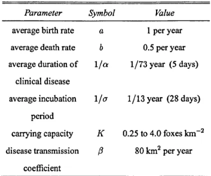
Parameter Symbol Value

average birth rate a 1 per year average death rate b 0.5 per year average duration of 1/0: 1/73 year (5 days)

clinical disease

average incubation

l/a

1/13 year (28 days) period

carrying capacity

K

0.25 to 4.0 foxes Ian-2 disease transmission (3 80 km2 per year

coefficient

Table 1.1: Values for the model parameters as given in Anderson et al. (1981).

was found, by determining when the basic reproductive rate is one, that a critical condition for the carrying capacity is

Kc= (0:+ a)(a+ a).

{3a (1.4)

K

>

Kc corresponds to the basic reproductive rate being greater than one resulting in rabies being maintained in the population.

Three types of behaviour are possible: For K

<

Kc rabies dies out and the susceptible popu-lation density tends to K, the diseas~free steady state value; if K

> Kc

rabies becomes endemic and the population densities oscillate about a steady state

8

=

8

0,1

=

10,

R

=

Ro.

These osciI-. lations are damped if K is not much bigger than Kc in which case the densities tend to the steady state.

A numerical analysis perfonned by Murray et al. (1986) shows that for the full system (D

#

0), if K

<

Kc rabies dies out. However, if K

>

Kc, then an epidemic wave fonns travelling with near-constant velocity.

The method of control employed by Murray et al. (1986) was to consider a barrier ahead of the epidemic wave where the susceptible population has been reduced below the critical density. This reduction can either be achieved through vaccination or culling, or a combination of the two. Estimates are made from the model (1.IHI.3) for the width of this break region and the level of reduction necessary. This method is being employed successfully both in Europe (MacKenzie, 1990, 1997) and Texas (Zoonosis Control Division, 1998).

In studying the control of the spread of rabies, it is implicit in the analysis carried out by Murray et al. (1986) that once the population reduction has occurred it is maintained at this level. Hence a control zone of vaccinated foxes ahead of an epizootic wave is treated as being equivalent to a region where the carrying capacity K has been reduced. In practice we would expect that, after the population reduction has been completed, the susceptible population would begin to recover and increase towards the environmental carrying capacity.

It has been argued (Harris and Smith, 1990) that the situation would be very different if ra-bies reached mainland Britain. Unlike in continental Europe where rara-bies is endemic and control strategies have to deal with an epizootic wave 2000 kilometres long, in Britain only a local, 'point-source' outbreak, would be experienced initially. A control strategy in Britain should, therefore, have the goals of both containing the outbreak and eliminating it in the original local area.

To study the problem of containing and eliminating point-source outbreaks; and to consider the recovery of the susceptible population we extend the model given by (1.IHl.3).

1.2.2 The extended model

ofvacci-nated animals in front of each wave front to prevent the further spread of the disease and to bring about its subsequent elimination. In the last year this has involved the aerial distribution of, on average, 10 000 baits per flight over the course of 254 flights.

With this in mind we can divide the control of rabies into three phases:

1. An input phase where the bait containing the vaccine is delivered. The control parameters are the trajectory of the deliverer and the amount deposited.

2. A vaccination phase where the bait is taken by the foxes and an immune response is produced msome.

3. An observation phase where we observe the effects of our control strategy.

We remark that culling could also be performed by the distribution of bait, substituting poison for vaccine (see, for example, Harris and Smith, 1990).

The first phase can either be performed by the manual placement or aerial distribution of bait. The speed of distribution depends on the delivery method and the area over which bait is dis-tributed. For example, the 1998 vaccination program carried out in Texas lasted for 34 days over a region of 108 780 square kilometres and involved the distribution of 2.6 million baits.

If the delivery of the bait is fast compared with the time frame of the rest of the dynamics the control or input to the system is the initial distribution (in space) of the bait. Suppose that the density of bait is B then a possible fonn for the dynamics of the bait is

BB

at

= - ("IsS

+

"III

+

"IvV) B - HB, (1.5)

where V is the density of vaccinated foxes; "Is, "II and "Iv measure the rate at which susceptible (respectively incubating, vaccinated) foxes take the bait; H is an increasing function in t and models the decomposition of the bait. To allow for environmental heterogeneity this function could be made spatially dependent.

virus, the virus dies out after a few weeks in the field. To maximise the useful life expectancy of the vaccinated baits they are currently distributed in Spring and Autumn (MacKenzie, 1990).

In the second phase susceptible foxes take the bait and an immune response is produced in some. Suppose that the susceptible foxes take the bait and become immune at an average rate per head of, B. If we suppose that vaccinated foxes give birth to susceptible ones so that immunity is not inherited, and that the vaccine does not produce any behavioural changes the dynamics of the susceptible class of fox becomes

as

(N)

7ft

=

(a -

b) 1-K S - {3RS - ,ES

+

aVo

(1.6)

The bait used in the Texas program also contains a biomark agent. This has been used to indicate bait uptake. Following the 1996 program this marker was found in 35% of a representative sample of grey foxes. Of this sample 32% showed a positive response. In Europe typically 70% of foxes in the target areas take the bait (MacKenzie, 1990).

Ifwe assume that incubating foxes do not become immune by taking the bait then the dynamics of [ and

R

remain unchanged; foxes in the clinical phase cannot be vaccinated against rabies. Therefore the remaining equations of the extended model are

av

(

N)

- = ,ES - b

+

(a -

b) - V

at

K (1.7)

ill (

N)

- =

{3RS - a[ - b

+

(a - b) - [

at

K (1.8)

aR

(

N)

2

at

=a[-aR-

b+(a-b)

K

R+DV R,

(1.9)

where

N

=

S

+

V

+ [ +

R

is the total fox population density.

A similar extension in the spatially uniform case can be found in Anderson et al. (1981), though we do not consider a rate of vaccination. We are dealing with the situation where bait is laid down and produces a level of vaccination which is allowed to have an effect. Possibly this program is repeated at a later stage, for example each year.

we need to produce in order to contain and eliminate an outbreak of rabies. Thus the simplified version of the system of equations (1.5)-( 1.9) that we consider in the following is

as

(N)

-=(a-b)

1 - -

S-(3RS+aV

at

K (1.10)

-

av

= -

(

b

+

(a -

b) -

N)

V

at

K

(1.11)

-=(3RS-aI-

aI

(

b+(a-b)- I

N)

at

K (1.12)

aR

(( N)

2

at

=

a

I - o:R -

b

+

a -

b) K R

+

DV R,

(1.13)

Our control or input to this system is the level of vaccination (or cull). This is the initial distribution (in space) of the vaccinated class produced by some baiting strategy. This poses an interesting and novel control problem. Usually in engineering control systems the control acts continuously in time throughout the period considered. Therefore in tackling this problem we must deal with a new style of control system.

1.3 Analysis of extended model

In this section we analyse the steady states of (1.10)-(1.13) for the spatially uniform case and compare the results with those obtained by Murray et al. (1986). In a similar fashion we first introduce non-dimensionalised quantities. We conclude the section with an interesting analysis of the time-varying nature of a vaccination procedure.

1.3.1 Analysis of steady states

It is helpful for the analysis of the steady states to introduce non-dimensionalised quantities for the model. We make the following substitutions:

s

=

S/K,v

=

V/K,q

=

I/K,r

=

R/K,n

=

N/K,

f =

(a - b)/f3K,

8

=

b/f3K,/-t

=

a/(3K,

22

CHAPTER 1. THE CONTROL PROBLEM

These quantities are along the lines of those introduced in Murray et al. (1986). With these substi-tutions the model becomes, on dropping the bar notation for simplicity,

8s

at

=f(l-n)s+(f+())v-rs (1.14) 8v

8t

=

-«()

+

fn)v (1.15)

8q

at

=

rs - (p

+ () +

fn)q (1.16)

8r

82_r

at

= pq - (d

+

fn)r

+

8x_{2 '} (1.17)

For the spatially uniform case we set ~

=

O. The steady states satisfy

s

=

v

=

q

=

r

=

0. We see immediately from equation (1.15) that

v

=

0 for a steady state. Therefore equations (1.14}-( 1.17) reduce to

at a steady state.

S = f(1 - n)s - rs

=

0

q

=

rs -

(p

+ () +

fn)q

=

0

r

=

/Lq -

(d

+

fn)r

=

O.

(1.18) (1.19) (1.20)

Two possible solutions are s = q

=

r = 0 and s

=

1, q

=

r

=

O. These correspond to the population free and disease free steady states respectively. To find the disease persistent steady state we assume that q

=I

0, and r

=I

O. Dividing (1.18) through by S gives

r = f (1- n),

and in particular n

=I

1 since r

=I

O. Now (1.20) yields

f

q = -

(d

+

fn) (1 -

n)

/L

and, upon substitution, (1.19) becomes 1

s = - (p

+ () +

fn)( d

+

fn) . /L

Therefore adding these equations together gives the following formula for

n.,

the total population density at the disease persistent steady state:

d (p

+ () +

f)

+

pf

n.

= .

Thus the disease persistent steady state is given by

(8.,

0, q.,

r.)

where

Murray et aI. (1986) made the observation that f, 6

«

1 and so performed an asymptotic analysis. In agreement with this analysis, to first order in f and 6,

S.,

q.,

r.

are given by

S. = d

+

~c5

+

d

(1

+~)

f

d

q. = -(1- d)f I-"

r.

=

(1 - d)f,

We now determine when this steady state is realistic-that is, when each of

S.,

q., r. is nonnegative. Since r.

oj:

0 we see that r. is realistic when

(1- (d(I-"+6 _J.t-f(6+f)

+

f)

+

I-"f))

>

O.

We expect J.t

>

f

(c5

+

f) since f and

c5

are small and so this inequality simplifies to

which can be rewritten in the form

[

c5

]-1

d< 1+

:f

- f ,

Similarly for q. to be realistic when (1.25) is satisfied the following condition must hold:

Again this simplifies to, assuming that I-"

> f (c5

+

f),

24 CHAPTER 1. THE CONTROL PROBLEM

which is clearly satisfied. Finally, for

s.

to be realistic the following condition must be satisfied:

This will be the case, provided J.-t

>

€ (c5

+

f),

if

Since c5 is small we expect that the right-hand side of this equation is negative; this occurs when - J.-t2 - J.-tc5 (1 - € )

+

c52

+

€2

<

O. Now since d

>

0 we see that the steady state is realistic if condition (1.25) holds. It now remains to check the stability of the system at each of the steady states.

Consider the general dynamical system

"2

=

J(z).

Suppose that the function

J

is differentiable with respect to

z.

Then making the substitution

z

=

z

+

Zo we have

z

=

J(zo)

+

:(zo)z

+

J(z) - zo·

Therefore, if Zo is a steady state and

IIzll

small,

dJ

-

-z

=

dZ(zo)z

+

J(z)

=

Az

+

J(z}.

The following well-known result gives a sufficient criterion for the stability of a steady state.

Theorem 1.3.1. Consider the general differential equation given by

"2

=

J(z).

Suppose that

J

is differentiable and

a(A)

C C_. Then the steady state is asymptotically stable.

Suppose that

f

is given by the equations (1.18)-(1.20), with

z

=

(s, v,

q, r)T and that Zo

=

(so,

0,

qo,

ro) T is the steady state under consideration. Then

E(1 - no) - SOE -

ro -fSo

+

(f

+

6)

- f80 -80(f

+

1)

df 0

-(6

+

fno) 0 0

ctz(zo)

=

ro - fqo

-Eqo

-(J-L

+

6

+

Eno) -

fqo

So -

fqo

-fro -ffo I-" - ffo

-(d

+

fno) - ffO

where

no

=

So

+

qo

+

ro. We will consider each of the three steady states in turn.

Zo

=

(0,0,0,0)

For this steady state the matrix A is given by

o

o

o

-6 0 0

o

0

-(J-L+6)

0

o

0 I-" -d

We see immediately that one of the eigenvalues is real and positive. Therefore this steady state is unstable.

Zo =

(1,0,0,0)

For this steady state the matrix

A

is given by

-f 6 -f -(f

+

1)

o

-(8

+

f)

0

0

o

0 - (I-"

+

0"

+

f)

1

o

0 I-"

-(d+d

By inspection we see that two of the eigenvalues are real and negative. The other two eigenvalues are roots of

Necessary and sufficient conditions for the roots to have negative real part are provided by the

Routh-Hurwitz conditions (Murray, 1993). These conditions are, for equation (1.26),

/-l

+

2€

+

0

+

d

>

0, and

The first equation is automatically satisfied since each of the parameters is positive. The second equation yields the following necessary and sufficient condition for the steady state to be stable

Zo

=

(s.,

0, q.,

r.)

For this steady state the matrix

A

is given by €(l -

n.) -

S.€ - T. -€S.

+

(€

+ 0)

o

-(0

+

fn.)

-€T.

-fS.

o

-S.(f

+

1)

o

-(/-l

+

0

+

€n.) - €q.

S. - €q.

/-l-

fT. -(d

+

€n.) - €T.

(1.27)

where

n.,

S., q., T. are given by equations (1.21) and (1.22)-(1.24). Two of the eigenvalues of this

matrix are

with the remaining eigenvalues being the roots of the following polynomial:

A2

+

A (d

+

€

(2n.

+

T.

+

q.)

+

0

+

/-l)

+

(/-l

+

0

+

f

(n.

+

q.))

(d

+

€

(n.

+

T.)) - (€T. -

/-l) (€q. -

s.).

Clearly

A2

<

0 and

Al

is given by

Al

=

€(1 -

n.) -

€S. - T. = -fS.

< 0,

(by (l.18) and the fact that S. =f. 0). Therefore it only remains to check whether the two roots of

roots have negative real part if and only if

and

The first of these conditions is clearly satisfied. For the second condition we expand out the terms to get

2 2 2 2

+

€

n.

+

€

n.r.

+

€

n.q.

+

€r.s.

+

€pq. -

P8 •.

Now s.

=

!(p

+

6

+

fn)(d

+

fn) and substituting for the last term gives

which is clearly positive. Hence this steady state is stable.

Remark 1.3.2. Recall that this steady state is realistic if condition (1.25) is satisfied which means that (1.27) is violated. Hence this steady state is realistic (and stable) if the disease free steady state is unstable. This is the requirement for an epidemic.

The condition (1.27) is the non-dimensionalised version of (1.4) and determines whether an epidemic will be maintained.

1.3.2 Some remarks

The analysis of the previous subsection is not unexpected. By including the vaccinated class of fox, with its time-dependence, rather than reducing the environmental carrying capacity, we do not change the stability of the system. Intuitively, if

K

>

Kc

(or in non-dimensionalised form

d

<

[1

+

~]

-1 - f), once the population density of the vaccinated class of fox has been reduced

Roughly speaking, while the population density of the susceptible class is less than K_{e ,} the system is stable in the sense that the infected population density will decrease. Once the susceptible population density has risen above K_{e ,} the system becomes unstable in the sense that an epidemic will begin and rabies will be maintained in the fox population.

We must remark at this stage a problem associated with using classical diffusion to model dispersal and continuous densities for populations of individuals. Both Kallen et a1. (1985) and Murray et a1. (1986) point out that mathematically the infected population density will always be positive everywhere and for all later times. This means that we must be careful in our analysis of the above extended model since mathematically if

K

>

Kc

whatever our vaccination program is, an epidemic will occur at some later point. The problem of continuous densities can be overcome by setting

R

= 0 (or

1=

0) if

R

(l respectively) is small enough.

1.3.3 Time dependence of vaccination procedures

Once a baiting trial has been completed and all of the bait has either been taken by foxes or decomposed the vaccinated population density will decrease. The susceptible population density will increase as vaccinated foxes give birth to susceptible ones. A critical question therefore for us to ask is: When will the density of the susceptible population be greater than or equal to the critical carrying capacity for an epidemic? If the outbreak of rabies has not been eliminated before this density has risen to this critical value an epidemic will occur.

To illustrate the problem of the recovery of the susceptible population density after a vaccina-tion has been carried suppose that a fox populavaccina-tion has reached the environmental carrying capacity

K, which is a steady state for the fox population in the absence of rabies.

After a baiting trial suppose that a proportion, A, of the susceptible foxes have been vaccinated. In the absence of any infected foxes the model equations (1.10)-(1.13) become

d8

_dt

₌

_{(a - b)}

(8+

_1-

_K

V)

₈

₊

_{aV, 8(0) = (1 - )")K}

dV

(

8+V)

di=-

b+(a-b) K

V,

V(O) = )"K.

(Days) 0.9 215 0.8 172 0.7 123 0.6 67

Table 1.2: Recovery of susceptible population density for a carrying capacity of 2 foxes krn -1 and a critical carrying capacity of 1 fox krn-I.

A

Tc

(Days) 0.9 51 0.8 8

Table 1.3: Recovery of susceptible population density for a carrying capacity of 4.6 foxes krn-1 and a critical carrying capacity of 1 fox krn-I.

all times t. Therefore

which has the solution

dS

-

=a(K-S)

dt

S(t)

=

K(l - Ae-at).

We are interested in the time

Tc

when

S(Tc)

=

_Kc,

the critical carrying capacity for an epidemic. This occurs at

We note from the results in Table 1.3 that in the U.K. a minimum reduction of 80% is required and then the system remains stable for only eight days. This means that the rabies has to be eliminated in eight days or an epidemic will occur. This has serious repercussions if an outbreak of rabies occurs in Britain.

These results seem to suggest that the time-dependence of the vaccination procedure is impor-tant when considering the efficacy of a control strategy.

1.4 Mathematical formulation of the control problem

Suppose that we wish to formulate the system of partial differential equations (1.1O}-(1.13) as an abstract differential equation. To do this let

n

c

~.2 be closed and bounded where

n

is the spatial domain. We set s(t) = S(t, .), v(t)

=

V(t, .), q(t)

=

J(t, .), r(t)

=

R(t, .), where, for example,

S(t,·)

=

{S(t,x): x

E S1}. Now fonn the vector

and consider the dynamics

where

f(·)

is given by (1. 1O}-(1. 13).

z(·)

=

s(.) v(·)

q(.)

r(·)

i

=

f(z)

(1.28)

The mechanism for controlling the spread of rabies considered in this thesis is population reduction. We allow for this reduction to be carried out in three ways: through a vaccination program; a cull; or a combined scheme of vaccination and culling.

So, qo,

and fo, then the initial condition for (1.28) is

So -1

0 1

z(O)

=

₊

Ul = Zo

+

BlUl' (1.29)

lio

0

fo 0

For the second method we suppose that an initial distribution, U2(') E PC(O;

lR),

of foxes has been culled. Then the initial condition for (1.28) is

So

-1

0 0

z(O) =

₊

U2 = Zo

+

B2u2. (1.30)

lio

0

fo 0

Clearly these two methods of population reduction can be combined to give a third scheme for controlling the spread of rabies. In this case we suppose that initial distributions Ul, and U2 of

foxes have been vaccinated and culled respectively. Then the initial condition for (1.28) is

So -1 -1

0 1 0

( : ) =zo+Bu.

z(O)

=

₊

(1.31)

7io

0 0

fo 0 0

For the purposes of reducing the total infected population density we consider the following observation

Controllability via the Initial State

The control problem which this thesis aims to solve is to drive some part, or all, of a particular biological or medical process, to some desired state in a specified time. The main application considered throughout this thesis is controlling the spread of rabies in a fox population. In this case the parts of the system that one wishes to control are the population densities of the incubating and rabid foxes. The novelty of these systems is that the control acts only through the initial state.

In Chapter 1 the control problem was formulated mathematically as an abstract differential equation. The part of the state that is to be controlled is formulated as an output so that the problem becomes that of driving the output of the system to a desired value in a specified time. In this chapter the important question ofwhether a solution to the mathematical control problem exists is considered. A weakening of the aim of the control problem leads to a positive answer. More satisfactorily it is shown that, under certain circumstances, if a solution exists then the method used

in this chapter will determine it.

The mathematical formulation of the control problem is as follows. Consider the abstract differential equation given by

i(t) = f(t, z(t))

the initial state is given by

z(O) = Z~

+

Bu.

The controls are assumed to belong to a Hilbert space U such that B E £(U, Z). Therefore the treatment of this thesis is confined to the situation involving bounded inputs. If, for the underlying system, it is not possible to affect the state at every point of the spatial domain so that the controls are restricted to only a few points or parts of the boundary the resulting model will involve an

unbounded input operator. Pritchard and Salamon (1987) considered systems with unbounded

inputs and outputs. In this case it is assumed that there exists a Banach space Z C Zl with continuous injection and dense range. The input operator is then assumed to be bounded from U

toZl •

The output associated with the differential equation is given by

y = Cz(T),

where

T

is the specified time and the output takes values in a Hilbert space

Y.

Mathematically the control problem is to choose u such that the resulting output is Y = Yd, the desired target output.

Again, if the part of the system that is to be controlled, that is the output, is the state at only certain points in the spatial domain or parts of the boundary the resulting model will have an unbounded output operator. If, in the rabies model, it was desired only to contain the spread of infection by keeping the density of infected foxes low on the boundary of the spatial domain, this would lead to an unbounded output operator. However in this thesis the aim is to reduce the infected population throughout the spatial domain.

Suppose that an initial guess is made for the control,

u'

say, with associated differential equation

Z'(t)

=

f(t, z'(t)),

Z'(O)

= z~

+

Bu', (2.1)

to get

i{t)

+

i'{t)

=

f{t, z{t)

+

z'{t)),

z{o)

=

z~

+

Bu

+

Bu' - z'{O).

(2.2)

Now suppose that

f

is differentiable around the trajectory

Ht, z'{t)) : t

E

[0,

T]}

in the sense that

f{t,

z) =

f(t, z'{t))

+

A{t)

(z -

z'{t))

+

D{t)N{t, E{t)(z - z'(t)))

(2.3)

for some piecewise continuous

A(·)

such that

A(t)

is an unbounded linear operator on Z for each t E

[0,

T];

DO

and E(·) characterise and describe the unboundedness of the nonlinear-ity. Therefore in the following it will be assumed that there are Banach spaces Z and Z such that

Z C Z C Z where the injections are continuous with dense ranges. With respect to these spaces we suppose that

D(t)

and

E{t)

are bounded (and so can be considered as unbounded operators with respect to Z). To give greater flexibility in the treatment of the nonlinearity we suppose that

N :

[0,

T] x W ----t W where W

C

W are Banach spaces. More precise assumptions will be introduced in the following.

Equation (2.2) can be rewritten as

i(t)

=

A(t)z(t)

+

D{t)N(t, E{t)z(t)),

z{O)

=

Bu.

(2.4)

The following assumption is made for the general differential equation.

Assumption 1 The initial guess for the control u' gives rise to a continuously differentiable (with respect to Z) solution z'(-) of(2.1). The nonlinear function

f

satisfies (2.3) with respect to this solution.