Sweeping through the Topic Space: Bad luck? Roll again!

Sweeping through the Topic Space:

Bad luck? Roll again!

Martin Riedl and Chris Biemann

Ubiquitous Knowledge Processing Lab

Computer Science Department, Technische Universit¨at Darmstadt Hochschulstrasse 10, D-64289 Darmstadt, Germany

[email protected], [email protected]

Abstract

Topic Models (TM) such as Latent Dirich-let Allocation (LDA) are increasingly used in Natural Language Processing applica-tions. At this, the model parameters and the influence of randomized sampling and inference are rarely examined — usually, the recommendations from the original

pa-pers are adopted. In this paper, we

ex-amine the parameter space of LDA topic models with respect to the application of Text Segmentation (TS), specifically target-ing error rates and their variance across dif-ferent runs. We find that the recommended settings result in error rates far from opti-mal for our application. We show substan-tial variance in the results for different runs of model estimation and inference, and give recommendations for increasing the robust-ness and stability of topic models. Run-ning the inference step several times and se-lecting the last topic ID assigned per token, shows considerable improvements. Similar improvements are achieved with the mode method: We store all assigned topic IDs during each inference iteration step and se-lect the most frequent topic ID assigned to each word. These recommendations do not only apply to TS, but are generic enough to transfer to other applications.

1 Introduction

With the rise of topic models such as pLSI (Hof-mann, 2001) or LDA (Blei et al., 2003) in Nat-ural Language Processing (NLP), an increasing number of works in the field use topic models to map terms from a high-dimensional word space

to a lower-dimensional semantic space. TMs

are ’the new Latent Semantic Analysis’ (LSA),

(Deerwester et al., 1990), and it has been shown that generative models like pLSI and LDA not only have a better mathematical foundation rooted in probability theory, but also outperform LSA in document retrieval and classification, e.g. (Hof-mann, 2001; Blei et al., 2003; Biro et al., 2008). To estimate the model parameters in LDA, the ex-act computation that was straightforward in LSA (matrix factorization) is replaced by a randomized Monte-Carlo sampling procedure (e.g. variational Bayes or Gibbs sampling).

Aside from the main parameter, the number of topics or dimensions, surprisingly little atten-tion has been spent to understand the interac-tions of hyperparameters, the number of sam-pling iterations in model estimation and inter-ference, and the stability of topic assignments across runs using different random seeds. While progress in the field of topic modeling is mainly made by adjusting prior distributions (e.g. (Sato and Nakagawa, 2010; Wallach et al., 2009)), or defining more complex model mixtures (Heinrich, 2011), it seems unclear whether improvements, reached on intrinsic measures like perplexity or on application-based evaluations, are due to an improved model structure or could originate from sub-optimal parameter settings or literally ’bad luck’ due to the randomized nature of the sam-pling process.

has been shown that this task considerably bene-fits from the use of TMs, see (Misra et al., 2009; Sun et al., 2008; Eisenstein, 2009).

This paper is organized as follows: In the next section, we present related work regarding text segmentation using topic models and topic model parameter evaluations. Section 3 defines the Top-icTiling text segmentation algorithm, which is a simplified version of TextTiling (Hearst, 1994), and makes direct use of topic assignments. Its simplicity allows us to observe direct conse-quences of LDA parameter settings. Further, we describe the experimental setup, our application-based evaluation methodology including the data set and the LDA parameters we vary in Section 4. Results of our experiments in Section 5 indi-cate that a) there is an optimal range for the num-ber of topics, b) there is considerable variance in performance for different runs for both model es-timation and inference, c) increasing the number of sampling iterations stabilizes average perfor-mance but does not make TMs more robust, but d) combining the output of several independent sam-pling runs does, and additionally leads to large er-ror rate reductions. Similar results are obtained by e) the mode method with less computational costs using the most frequent topic ID that is assigned during different inference iteration steps. In the conclusion, we give recommendations to add sta-bility and robustness for TMs: aside from opti-mization of the hyperparameters, we recommend combining the topic assignments of different in-ference iterations, and/or of different independent inference runs.

2 Related Work

2.1 Text Segmentation with Topic Models

Based on the observation of Halliday and Hasan (1976) that the density of coherence relations is higher within segments than between segments, most algorithms compute a coherence score to measure the difference of textual units for inform-ing a segmentation decision. TextTilinform-ing (Hearst, 1994) relies on the simplest coherence relation – word repetition – and computes similarities be-tween textual units based on the similarities of word space vectors. The task of text segmenta-tion is to decide, for a given text, how to split this text into segments.

Related to our algorithm (see Section 3.1) are the approaches described in Misra et al. (2009) and Sun et al. (2008): topic modeling is used to alleviate the sparsity of word vectors by mapping words into a topic space. This is done by extend-ing the dynamic programmextend-ing algorithms from (Utiyama and Isahara, 2000; Fragkou et al., 2004) using topic models. At this, the topic assignments have to be inferred for each possible segment.

2.2 LDA and Topic Model Evaluation

For topic modeling, we use the widely applied LDA (Blei et al., 2003), This model uses a train-ing corpus of documents to create document-topic and topic-word distributions and is parameterized

by the number of topics T as well as by two

hyperparameters. To generate a document, the topic proportions are drawn using a Dirichlet

dis-tribution with hyperparameter α. Adjacent for

each word w a topiczdw is chosen according to

a multinomial distribution using hyperparameter

βzdw. The model is estimated using m

itera-tions of Gibbs sampling. Unseen documents can be annotated with an existing topic model using Bayesian inference methods. At this, Gibbs sam-pling withiiterations is used to estimate the topic ID for each word, given the topics of the other words in the same sentential unit. After inference, every word in every sentence receives a topic ID, which is the sole information that is used by the TopicTiling algorithm to determine the segmenta-tion. We use the GibbsLDA implementation by Phan and Nguyen (2007) for all our experiments. The article of Blei et al. (2003) compares LDA with pLSI and Mixture Unigram models using the perplexity of the model. In a collaborative filter-ing evaluation for different numbers of topics they observe that using too many topics leads to over-fitting and to worse results.

In Wallach et al. (2009) topic models are eval-uated with symmetric and asymmetric hyperpa-rameters based on the perplexity. They observe

a benefit using asymmetric parameters forα, but

cannot show improvement with asymmetric priors forβ.

3 Method

3.1 TopicTiling

For the evaluation of the topic models, a text seg-mentation algorithm called TopicTiling is used here. This algorithm is a newly developed al-gorithm based on TextTiling (Hearst, 1994) and achieves state of the art results using the Choi dataset, which is a standard dataset for TS eval-uation. The algorithm uses sentences as minimal units. Instead of words, we use topic IDs that are assigned to each word using the LDA infer-ence running on sentinfer-ence units. The LDA model should be estimated on a corpus of documents that is similar to the to-be-segmented documents.

To measure the coherencecp between two

sen-tences around position p, the cosine similarity

(vector dot product) between these two adjacent sentences is computed. Each sentence is

repre-sented as aT-dimensional vector, whereT is the

number of topic IDs defined in the topic model.

The t-th element of the vector contains the

num-ber of times thet-th topic is observed in the sen-tence. Similar to the TextTiling algorithm, lo-cal minima lo-calculated from these similarity scores are taken as segmentation candidates.

This is illustrated in Figure 1, where the simi-larity scores between adjacent sentences are plot-ted. The vertical lines in this plot indicate all local minima found.

0 5 10 15 20 25 30

0.0

0.2

0.4

Sentence

cosine similar

ity

Figure 1: Cosine similarity scores of adjacent sen-tences based on topic distribution vectors. Vertical lines (solid and dashed) indicate local minima. Solid lines mark segments that have a depth score above a chosen threshold.

Following the TextTiling definition, not the minimum scorecp at positionpitself is used, but

a depth scoredpfor positionpcomputed by

di= 1/2∗(cp−1−cp+cp+1−cp). (1)

In contrast to TextTiling, the directly neighboring similarity scores of the local minima are used, if they are higher thancp. When using topics instead

of words, it can be expected that sentences within one segment have many topics in common, which leads to cosine similarities close to1. Further, us-ing topic IDs instead of words greatly increases

sparsity. A minimum in the curve indicates a

change in topic distribution. Segment boundaries

are set at the positions of the n highest

depth-scores, which is common practice in text

segmen-tation algorithms. An alternative to a given n

would be the selection of segments according to a depth score threshold.

4 Experimental Setup

As dataset the Choi dataset (Choi, 2000) is used. This dataset is an artificially generated corpus that consists of 700 documents. Each document

con-sists of 10 segments and each segment has 3–

11 sentences extracted from a document of the Brown corpus. For the first setup, we perform a 10-fold Cross Validation (CV) for estimating the TM (estimating on 630 documents at a time), for the other setups we use 600 documents for TM estimation and the remaining 100 documents for testing. While we aim to neglect using the same documents for training and testing, it is not guar-anteed that all testing data is unseen, since the same source sentences can find their way in sev-eral artificially crafted ’documents’. This prob-lem, however, applies for all evaluations on this dataset that use any kind of training, be it LDA models in Misra et al. (2009) or TF-IDF values in Fragkou et al. (2004).

For the evaluation of the Topic Model in

combi-nation of Text Segmentation, we use thePk

mea-sure (Beeferman et al., 1999), which is a stan-dard measure for error rates in the field of TS. This measure compares the gold standard seg-mentation with the output of the algorithm. A

Pk value of 0 indicates a perfect segmentation,

the averaged state of the art on the Choi Dataset

is Pk = 0.0275 (Misra et al., 2009). To assess

configurations of the LDA model, and plot the re-sults using Box-and-Whiskers plots: the box in-dicates the quartiles and the whiskers are maxi-mal 1.5 times of the Interquartile Range (IQR) or equal to the data point that is no greater to the 1.5 IQR. The following parameters are subject to our exploration:

• T: Number of topics used in the LDA model.

Common values vary between 50 and 500.

• α: Hyperparameter that regulates the

sparse-ness topic-per-document distribution. Lower values result in documents being represented by fewer topics (Heinrich, 2004).

Recom-mended: α = 50/T (Griffiths and Steyvers,

2004)

• β : Reducing β increases the sparsity of

topics, by assigning fewer terms to each topic, which is correlated to how related words need to be, to be assigned to a topic

(Heinrich, 2004). Recommended: β =

{0.1,0.01} (Griffiths and Steyvers, 2004; Misra et al., 2009)

• m Model estimation iterations.

Recom-mended / common settings:m= 500−5000

(Griffiths and Steyvers, 2004; Wallach et al., 2009; Phan and Nguyen, 2007)

• iInference iterations. Recommended /

com-mon settings:100(Phan and Nguyen, 2007)

• d Mode of topic assignments. At each

in-ference iteration step, a topic ID is assigned to each word within a document (represented as a sentence in our application). With this option, we count these topic assignments for each single word in each iteration. After alli

inference iterations, the most frequent topic ID is chosen for each word in a document.

• r Number of inference runs: We repeat the

inference r times and assign the most

fre-quently assigned topic per word at the fi-nal inference run for the segmentation

algo-rithm. High r values might reduce

fluctua-tions due to the randomized process and lead to a more stable word-to-topic assignment.

All introduced parameters parameterize the TM. We are not aware of any research that has used

several inference runsrand the mode of topic

as-signmentsdto increase stability and varying TM

parameters in combinations with measures other then perplexity.

5 Results

In this section, we present the results we obtained from varying the parameters under examination.

5.1 Number of TopicsT

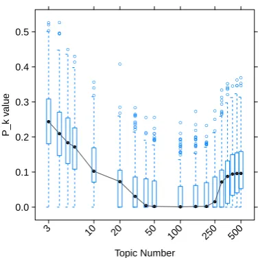
To provide a first impression of the data, a 10-fold CV is calculated and the segmentation results are visualized in Figure 2.

Topic Number P_k v alue 0.0 0.1 0.2 0.3 0.4 0.5

3 _{10 20 50}

100 250 500

● ● ● ● ● ● ● ●● ● ● ●● ● ●● ●● ● ● ● ● ● ● ● ● ● ● ● ● ● ● ● ● ● ● ● ● ● ● ● ● ● ● ● ● ● ● ● ● ● ● ● ● ● ● ● ● ● ● ● ● ● ● ● ● ● ● ● ● ● ● ● ● ● ● ● ● ● ● ● ● ● ● ● ● ● ● ● ● ● ● ● ● ● ● ● ● ● ● ● ● ● ● ● ● ● ● ● ● ● ● ● ● ● ● ● ● ●● ● ●

Figure 2: Box plots for different number of topicsT.

Each box plot is generated from the averagePk value

of 700 documents,α= 50/T,β = 0.1,m = 1000,

i= 100, r = 1. These documents are segmented with TopicTiling using a 10-folded CV.

Each box plot is generated from the Pk values

of 700 documents. As expected, there is a contin-uous range of topic numbers, namely between 50

and 150 topics, where we observe the lowestPk

values. Using too many topics leads to overfitting of the data and too few topics result in too gen-eral distinctions to grasp text segments. This is in line with other studies, that determine an optimum forT, cf. (Griffiths and Steyvers, 2004), which is specific to the application and the data set.

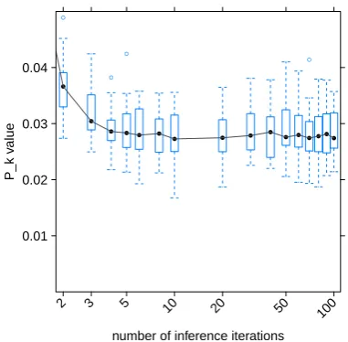
5.2 Estimation and Inference iterations

that is applied by TopicTiling to segment the re-maining 100 documents. From Figure 2 we know that sampling 100 topics leads to good results. To have an insight into unstable topic regions we also inspect performance at different sampling it-erations using 20 and 250 topics. To assess sta-bility across different model estimation runs, we trained 30 LDA models using different random seeds. Each box plot in Figures 3 and 4 is gen-erated from 30 mean values, calculated from the

Pk values of the 100 documents. The variation

indicates the score variance for the 30 different models.

Number of topics: 100

number of sample iterations

P_k v

alue

0.0 0.1 0.2 0.3 0.4

2 3 5 _{10 20 50}

100 _{300 500 1000}

● ● _{● ●}

●

●

●

●

●

●

●

●

● ● ● ● ● ● ● ● ● ● ● ● ●

● ●

●

●

●

● ●

0.02 0.04 0.06 0.08 0.10

50 _{100 300 500}

1000 ●

●

●

● _{● ●} ● ● ● ● ● ● ● ● ● ●

●

●

● ●

Figure 3: Box plots with different model estimation

iterationsm, withT=100,α = 50/T,β = 0.1,i =

100,r= 1. Each box plot is generated from 30 mean

values calculated from 100 documents.

Using 100 topics (see Figure 3), the burn-in

phase starts with 8–10 iterations and the meanPk

values stabilize after 40 iterations. But looking

at the inset for large m values, significant

vari-ations between the different models can be

ob-served: note that the Pk error rates are almost

double between the lower and the upper whisker. These remain constant and do not disappear for

largermvalues: The whiskers span error rates

be-tween 0.021 - 0.037 for model estimation on doc-ument units

With 20 topics, thePkvalues are worse as with

100 topics, as expected from Figure 2. Here the convergence starts at 100 sample iterations. More interesting results are achieved with 250 topics. A robust range for the error rates can be found be-tween 20 and 100 sample iterations. With more

iterations m, the results get both worse and

un-stable: as the ’natural’ topics of the collection have to be split in too many topics in the model, perplexity optimizations that drive the estimation process lead to random fluctuations, which the TopicTiling algorithm is sensitive to. Manual

in-spection of models forT = 250revealed that in

fact many topics do not stay stable across estima-tion iteraestima-tions.

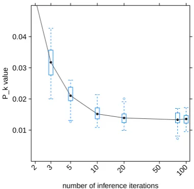
number of inference iterations

P_k v

alue

0.01 0.02 0.03 0.04

2 3 5 _{10 20 50}

100

●

●

● ● ● ●

● ● ● ● ● ●● ●●●

●

● ●

●

Figure 5: Figure of box plots for different inference

iterationsi and m = 1000, T = 100, α = 50/T,

β= 0.1,r= 1.

In the next step we sweep over several infer-ence iterationsi. Starting from 5 iterations, error rates do not change much, see Figure 5. But there is still substantial variance, between about 0.019 -0.038 for inference on sentence units.

5.3 Number of inference runsr

To decrease this variance, we assign the topic not only from a singe inference run, but repeat the in-ference calculations several times, denoted by the

parameterr. Then the frequency of assigned topic

IDs per token is counted across therruns, and we

assign the most frequent topic ID (frequency ties are broken randomly). The box plot for several evaluated values ofris shown in Figure 6.

This log-scaled plot shows that both variance

andPk error rate can be substantially decreased.

Already for r = 3, we observe a significant

im-provement in comparison to the default setting of

r= 1and with increasingrvalues, the error rates

are reduced even more: forr = 20, variance and

Number of topics: 20

number of sample iterations

P_k v

alue

0.1 0.2 0.3 0.4

2 3 5 _{10 20 50}

100 _{300 500 1000}

● ● ●

●_● ●

●

●

●

●

●

●

●

●

● ● ● ● ● ● ● ● ● ● ●

●

● ● ●

● ●

●

● ● ●

● ●

● ●

●

● 0.02

0.04 0.06 0.08 0.10

50 100 300 500 1000 ●

●

● ●

● ● ● ● ● ● ● ● ● ●

● ●

●

● ●

● ● ●

● ●

●

●

Number of topics: 250

number of sample iterations

P_k v

alue

0.1 0.2 0.3 0.4

2 3 5 _{10 20 50}

100 _{300 500 1000}

● ● ● ●

● ●

●

●

●

●

●

●

● _●

● ● ● ●

● ● ● ●

● ● ●

● ●

●

● ●

●

●

●

● ●

● ● 0.02

0.04 0.06 0.08 0.10

50 100 300 500 1000 ●

●

● ●

● ●

● ●

●

● ● ● ●

● ● ●

●

● ●

● ●

Figure 4: Box plots with varying model estimation iterationsmapplied withT = 20(left) andT = 250(right)

topics,α= 50/T,β= 0.1,i= 100,r= 1

number of repeated inferences

P_k v

alue

0.01 0.02 0.03 0.04

1 3 5 _{10 20}

●

●

●

●

●

●

Figure 6: Box plot for several inference runsr, to

as-sign the topics to a word with m = 1000,i = 100,

T = 100,α= 50/T,β = 0.1.

5.4 Mode of topic assignmentd

In the previous experiment, we use the topic IDs that have been assigned most frequently at the last inference iteration step. Now, we examine some-thing similar, but for alliinference steps of a sin-gle inference run: we select the mode of topic ID assignments for each word across all inference steps. The impact of this method on error and variance is illustrated in Figure 7. Using a sin-gle inference iteration, the topic IDs are almost assigned randomly. After 20 inference iterations

Pkvalues below0.02are achieved. Using further

iterations, the decrease of the error rate is only

number of inference iterations

P_k v

alue

0.01 0.02 0.03 0.04

2 3 5 _{10 20 50}

100

●

●

●

● _● ●

●

●

●

Figure 7: Box plot using the mode methodd =true

with several inference iterationsiwithm= 500,T =

100,α= 50/T,β = 0.1.

marginal. In comparison to the repeated inference method, the additional computational costs of this method are much lower as the inference iterations have to be carried out anyway in the default appli-cation setting.

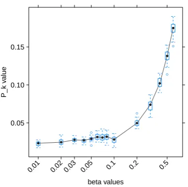
5.5 Hyperparametersαandβ

In many previous works, hyperparameter settings

α = 50/T andβ = {0.1,0.01} are commonly

used. In the next series of experiments we inves-tigate how different parameters of these both pa-rameters can change the TS task.

For α values, shown in Figure 8, we can see

0.5leads to sub-optimal results, and an error rate reduction of about 40% can be realized by setting

α = 0.1.

alpha values

P_k v

alue

0.01 0.02 0.03 0.04

0.01 0.02 0.03 0.05 0.1 0.2 0.5 1

● ● ● _●

● ●

● ●

●●

● ●

●

●

● ●

●

●

Figure 8: Box plot for several alpha valuesαwithm=

500,i= 100,T = 100,β= 0.1,r= 1.

Regarding values of β, we find that Pk rates

and their variance are relatively stable between the recommended settings of0.1and0.01. Values

larger than 0.1lead to much worse performance.

Regarding variance, no patterns within the stable range emerge, see Figure 9.

beta values

P_k v

alue

0.05 0.10 0.15

0.01 0.02 0.03 0.05 0.1 0.2 0.5

● ● ● ● ●

● ● ● _●

● ●

● ●

●

●

●

● ●

●

Figure 9: Box plot for several beta valuesβwithm=

500,i= 100,T = 100,α= 50/T,r= 1.

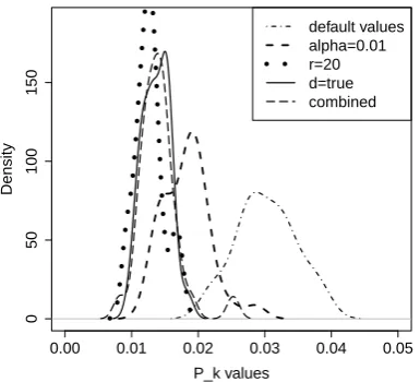
5.6 Putting it all together

Until this point, we have examined different pa-rameters with respect to stability and error rates one at the time. Now, we combine what we have

System Pk error σ2 var.

red. red.

default 0.0302 0.00% 2.02e-5 0.00%

α= 0.1 0.0183 39.53% 1.22e-5 39.77%

r= 20 0.0127 57.86% 4.65e-6 76.97%

d=true 0.0137 54.62% 3.99e-6 80.21%

combined 0.0141 53.45% 9.17e-6 54.55%

Table 1: Comparison of single parameter

optimiza-tions, and combined system.Pkaverages and variance

are computed over 30 runs, together with reductions

relative to the default setting. Default:α= 0.5,r= 1.

combined:α= 0.1,r= 20,d=true

learned from this and strive at optimal system per-formance. For this, we contrast TS results ob-tained with the default LDA configuration with the best systems obtained by optimization of sin-gle parameters, as well as to a system that uses these optimal settings for all parameters. Table 1 showsPkerror rates for the different systems. At

this, we fixed the following parameters:T = 100,

m = 500,i = 100, β = 0.1. For the computa-tions we use 600 documents for the LDA model estimation, apply TopicTiling and compute the er-ror rate for the 100 remaining documents and re-peat this 30 times with different random seeds.

We can observe a massive improvement for

op-timized single parameters. The α-tuning tuning

results in an error rate reduction of 39.77% in comparison to the default configurations. Using

r = 20, the error rate is cut in less than half

its original value. Also for the mode mechanism

(d = true) the error rate is halved but slightly

worse than than when using the repeated infer-ence. Using combined optimized parameters does not result to additional error decreases. We at-tribute the slight decline of the combined method in both in the error ratePkand in the variance to

0.00 0.01 0.02 0.03 0.04 0.05

0

50

100

150

P_k values

Density

default values alpha=0.01 r=20 d=true combined

Figure 10: Density plot of the error distributions for the systems listed in Table 1

6 Conclusion

In this paper, we examined the robustness of LDA topic models with respect to the application of Text Segmentation by sweeping through the topic model parameter space. To our knowledge, this is the first attempt to systematically assess the sta-bility of topic models in a NLP task.

The results of our experiments are summarized as follows:

• Perform the inferencertimes using the same

model and choosing the assigned topic ID per word token taken from the last infer-ence iteration, improves both error rates and stability across runs with different random seeds.

• Almost equal performance in terms of

er-ror and stability is achieved with the mode mechanism: choose the most frequent topic ID assignment per word across inference steps. While error rates were slightly higher for our data set, this method is probably preferable in practice because of its lower computation costs.

• As found in other studies, there is a range for

the number of topics T, where optimal

re-sults are obtained. In our task, performance showed to be robust in the range of 50 - 150 topics.

• The default setting for LDA hyperparameters

αandβ can lead to sub-optimal results.

Es-peciallyαshould be optimized for the task at

hand, as the utility of the topic model is very sensitive to this parameter.

• While the number of iterations for model

es-timation and inference needed for conver-gence is depending on the number of topics, the size of the sampling unit (document) and the collection, it should be noted that after convergence the variance between different sampling runs does not decrease for a larger number of iterations.

Equipped with the insights gained from exper-iments on single parameter variation, we were able to implement a very simple algorithm for text segmentation that improves over the state of the art on a standard dataset by a large margin. At this, the combination of the optimalα, and a high

number of inference repetitions r and the mode

method (d=true) produced slightly more errors

than a highralone. While the purpose of this

pa-per was mainly to address robustness and stability issues of topic models, we are planning to apply the segmentation algorithm to further datasets.

The most important takeaway, however, is that especially for small sampling units like sentences, tremendous improvements in applications can be obtained when looking at multiple inference as-signments and using the most frequently assigned topic ID in subsequent processing – either across diffeent inference steps or across diffeent infer-ence runs. These two new strategies seem to be able to offset sub-optimal hyperparameters to a certain extent. This scheme is not only applica-ble to Text Segmentation, but in all applications where performance crucially depends on stable topic ID assignments per token. Extensions to this scheme, like ignoring tokens with a high topic variability (stop words or general terms) or dy-namically deciding to conflate several topics be-cause of their per-token co-occurrence, are left for future work.

7 Acknowledgments

References

D. Beeferman, A. Berger, and J. Lafferty. 1999.

Statistical models for text segmentation. Machine

learning, 34(1):177–210.

Istvan Biro, Andras Benczur, Jacint Szabo, and Ana Maguitman. 2008. A comparative analysis of la-tent variable models for web page classification. In

Proceedings of the 2008 Latin American Web Con-ference, pages 23–28, Washington, DC, USA. IEEE Computer Society.

David M. Blei, Andrew Y. Ng, and Michael I. Jordan.

2003. Latent dirichlet allocation. J. Mach. Learn.

Res., 3:993–1022, March.

Freddy Y. Y. Choi. 2000. Advances in domain

inde-pendent linear text segmentation. InProceedings of

the 1st North American chapter of the Association for Computational Linguistics conference, NAACL 2000, pages 26–33, Stroudsburg, PA, USA. Associ-ation for ComputAssoci-ational Linguistics.

Scott Deerwester, Susan T. Dumais, George W. Fur-nas, Thomas K. Landauer, and Richard Harshman.

1990. Indexing by latent semantic analysis.

Jour-nal of the American Society for Information

Sci-ence, 41(6):391–407.

Jacob Eisenstein. 2009. Hierarchical text

segmenta-tion from multi-scale lexical cohesion.Proceedings

of Human Language Technologies: The 2009 An-nual Conference of the North American Chapter of the Association for Computational Linguistics on -NAACL ’09, page 353.

P. Fragkou, V. Petridis, and Ath. Kehagias. 2004. A Dynamic Programming Algorithm for Linear Text

Segmentation. Journal of Intelligent Information

Systems, 23(2):179–197, September.

Thomas L. Griffiths and Mark Steyvers. 2004.

Find-ing scientific topics. PNAS, 101(suppl. 1):5228–

5235.

M A K Halliday and Ruqaiya Hasan. 1976. Cohesion

in English, volume 1 of English Language Series. Longman.

Marti a. Hearst. 1994. Multi-paragraph segmentation

of expository text. Proceedings of the 32nd annual

meeting on Association for Computational

Linguis-tics, (Hearst):9–16.

Gregor Heinrich. 2004. Parameter estimation for text analysis. Technical report.

Gregor Heinrich. 2011. Typology of

mixed-membership models: Towards a design method. InMachine Learning and Knowledge Discovery in Databases, volume 6912 ofLecture Notes in Com-puter Science, pages 32–47. Springer Berlin / Hei-delberg. 10.1007/978-3-642-23783-6 3.

Thomas Hofmann. 2001. Unsupervised Learning by

Probabilistic Latent Semantic Analysis. Computer,

pages 177–196.

Hemant Misra, Joemon M Jose, and Olivier Capp´e. 2009. Text Segmentation via Topic Modeling : An

Analytical Study. In Proceeding of the 18th ACM

Conference on Information and Knowledge Man-agement - CIKM ’09, pages 1553—-1556.

Xuan-Hieu Phan and Cam-Tu Nguyen. 2007.

GibbsLDA++: A C/C++

implementa-tion of latent Dirichlet allocation (LDA).

http://jgibblda.sourceforge.net/.

Issei Sato and Hiroshi Nakagawa. 2010. Topic mod-els with power-law using pitman-yor process

cate-gories and subject descriptors. Science And

Tech-nology, (1):673–681.

Qi Sun, Runxin Li, Dingsheng Luo, and Xihong Wu. 2008. Text segmentation with LDA-based Fisher

kernel. Proceedings of the 46th Annual Meeting

of the Association for Computational Linguistics on Human Language Technologies Short Papers - HLT

’08, (June):269.

Masao Utiyama and Hitoshi Isahara. 2000. A Statis-tical Model for Domain-Independent Text

Segmen-tation. Communications.

Hanna Wallach, David Mimno, and Andrew McCal-lum. 2009. Rethinking lda: Why priors matter. In