Learning the Optimal Use of Dependency parsing Information for Finding Translations with Comparable Corpora

Learning the Optimal use of Dependency-parsing Information for Finding

Translations with Comparable Corpora

Daniel Andrade†_{, Takuya Matsuzaki}†_{, Jun’ichi Tsujii}‡ †_{Department of Computer Science, University of Tokyo}

{daniel.andrade, matuzaki_}@is.s.u-tokyo.ac.jp

‡_{Microsoft Research Asia, Beijing} [email protected]

Abstract

Using comparable corpora to find new word translations is a promising approach for ex-tending bilingual dictionaries (semi-) auto-matically. The basic idea is based on the assumption that similar words have similar contexts across languages. The context of a word is often summarized by using the bag-of-words in the sentence, or by using the words which are in a certain dependency position, e.g. the predecessors and succes-sors. These different context positions are then combined into one context vector and compared across languages. However, previ-ous research makes the (implicit) assumption that these different context positions should be weighted as equally important. Furthermore, only the same context positions are compared with each other, for example the successor po-sition in Spanish is compared with the suc-cessor position in English. However, this is not necessarily always appropriate for lan-guages like Japanese and English. To over-come these limitations, we suggest to perform a linear transformation of the context vec-tors, which is defined by a matrix. We de-fine the optimal transformation matrix by us-ing a Bayesian probabilistic model, and show that it is feasible to find an approximate solu-tion using Markov chain Monte Carlo meth-ods. Our experiments demonstrate that our proposed method constantly improves transla-tion accuracy.

1 Introduction

Using comparable corpora to automatically extend bilingual dictionaries is becoming increasingly

pop-ular (Laroche and Langlais, 2010; Andrade et al., 2010; Ismail and Manandhar, 2010; Laws et al., 2010; Garera et al., 2009). The general idea is based on the assumption that similar words have similar contexts across languages. The context of a word can be described by the sentence in which it occurs (Laroche and Langlais, 2010) or a sur-rounding word-window (Rapp, 1999; Haghighi et al., 2008). A few previous studies, like (Garera et al., 2009), suggested to use the predecessor and suc-cessors from the dependency-parse tree, instead of a word window. In (Andrade et al., 2011), we showed that including dependency-parse tree context posi-tions together with a sentence bag-of-words context can improve word translation accuracy. However previous works do not make an attempt to find an optimalcombination of these different context posi-tions.

Our study tries to find an optimal weighting and aggregation of these context positions by learning a linear transformation of the context vectors. The motivation is that different context positions might be of different importance, e.g. the direct predeces-sors and succespredeces-sors from the dependency tree might be more important than the larger context from the whole sentence. Another motivation is that depen-dency positions cannot be always compared across different languages, e.g. a word which tends to oc-cur as a modifier in English, can tend to ococ-cur in Japanese in a different dependency position.

As a solution, we propose to learn the optimal combination of dependency and bag-of-words sen-tence information. Our approach uses a linear trans-formation of the context vectors, before comparing

10

them using the cosine similarity. This can be con-sidered as a generalization of the cosine similarity. We define the optimal transformation matrix by the maximum-a-posterior (MAP) solution of a Bayesian probabilistic model. The likelihood function for a translation matrix is defined by considering the ex-pected achieved translation accuracy. As a prior, we use a Dirichlet distribution over the diagonal ele-ments in the matrix and a uniform distribution over its non-diagonal elements. We show that it is fea-sible to find an approximation of the optimal so-lution using Markov chain Monte Carlo (MCMC) methods. In our experiments, we compare the pro-posed method, which uses this approximation, with the baseline method which uses the cosine similarity without any linear transformation. Our experiments show that the translation accuracy is constantly im-proved by the proposed method.

In the next section, we briefly summarize the most relevant previous work. In Section 3, we then ex-plain the baseline method which is based on previ-ous research. Section 4 explains in detail our posed method, followed by Section 5 which pro-vides an empirical comparison to the baseline, and analysis. We summarize our findings in Section 6.

2 Previous Work

Using comparable corpora to find new translations was pioneered in (Rapp, 1999; Fung, 1998). The ba-sic idea for finding a translation for a wordq(query),

is to measure the context ofq and then to compare

the context with each possible translation candidate, using an existing dictionary. We will call words for which we have a translation in the given dic-tionary, pivot words. First, using the source cor-pus, they calculate the degree of association of a query wordq with all pivot words. The degree of association is a measure which is based on the co-occurrence frequency of q and the pivot word in a

certain context position. A context (position) can be a word-window (Rapp, 1999), sentence (Utsuro et al., 2003), or a certain position in the dependency-parse tree (Garera et al., 2009; Andrade et al., 2011). In this way, they get a context vector for q, which

contains the degree of association to the pivot words in different context positions. Using the target cor-pus, they then calculate a context vector for each

possible translation candidate x, in the same way.

Finally, they compare the context vector of q with the context vector of each candidatex, and retrieve

a ranked list of possible translation candidates. In the next section, we explain the baseline which is based on that previous research.

The general idea of learning an appropriate method to compare high-dimensional vectors is not new. Related research is often called “metric-learning”, see for example (Xing et al., 2003; Basu et al., 2004). However, for our objective function it is difficult to find an analytic solution. To our knowl-edge, the idea of parameterizing the transformation matrix, in the way we suggest in Section 4, and to learn an approximate solution with a fast sampling strategy is new.

3 Baseline

Our baseline measures the degree of association be-tween the query wordq and each pivot word with

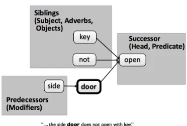
respect to several context positions. As a context position we consider the predecessors, successors, siblings with respect to the dependency parse tree, and the whole sentence (bag-of-words). The depen-dency information which is used is also illustrated in Figure 1. As a measure of the degree of association we use the Log-odds-ratio as proposed in (Laroche and Langlais, 2010).

Figure 1: Example of the dependency information used by our approach. Here, from the perspective of “door”.

context positioniwe define a vector qi which con-tains the degree of association with each pivot word in the context position i. If we number the pivot

words from 1 to n, then this vector can be

writ-ten as qi = (qi1, . . . , qin). Note that in our case i ranges from 1 to 4, representing the context posi-tions predecessors (1), successors (2), siblings (3), and the sentence bag-of-words (4). Finally, the com-plete context vector for the queryq is a long vector qwhich appends each qi, i.e.: q = (q1, . . . ,q4). Next, in the same way as before, we create a con-text vectorxfor each translation candidatex in the

target language. For simplicity, we assume that each pivot word in the source language has only one cor-responding translation in the target language. As a consequence, the dimensions of q andx are the same. Finally we can score each translation candi-date by using the cosine similarity betweenq and

x.

We claim that all of the context positions (1 to 4) can contain information which is helpful to identify translation candidates. However, we do not know about their relative importance, neither do we know whether these dependency positions can be com-pared across language pairs as different as Japanese and English. The cosine similarity simply weights all dependency position equally important and ig-nores problems which might occur when comparing dependency positions across languages.

4 Proposed Method

Our proposed method tries to overcome the short-comings of the cosine-similarity by using the fol-lowing generalization:

sim(q,x) = qAx

T √

qAqT√_xAxT , (1)

whereAis a positive-definite matrix inRdn×dn_{, and} T _{is the transpose of a vector. This can also be} con-sidered as linear transformation of the vectors using √

A before using the normal cosine similarity, see also (Basu et al., 2004).1

The challenge is to find an appropriate matrix A

which is expected to take the correlations between

1_{Therefore, exactly speaking A is not the transformation}

matrix, however it defines uniquely the transformation matrix

√

A.

the different dimensions into account, and which op-timally weights the different dimensions. Note that, if we set A to the identity matrix, we recover the

normal cosine similarity, which is our baseline. Clearly, finding an optimal matrix in Rdn×dn _is infeasible due to the high dimensionality. We will therefore restrict the structure ofA.

Let I be the identity matrix in Rn×n _{, then we} define the matrixA, as follows:

A=

   

d1I z1,2I z1,3I z1,4I

z1,2I d2I z2,3I z2,4I

z1,3I z2,3I d3I z3,4I

z1,4I z2,4I z3,4I d4I    

It is clear from this definition thatd1, . . . , d4weights the context positions1 to 4. Furthermore,zi,j can be interpreted as a the confusion coefficient between context positioniandj. For example, a high value for z2,3 means that a pivot word which occurs in the sibling position in Japanese (source language), might not necessarily occur in the sibling position in English (target language), but instead in the succes-sor position. However, in order to reduce the dimen-sionality of the parameter space further, we assume that each suchzi,j has the same valuez. Therefore, matrixAbecomes

A=

   

d1I zI zI zI

zI d2I zI zI

zI zI d3I zI

zI zI zI d4I     .

In the next subsection we will explain how we de-fine an optimal solution forA.

4.1 Optimal solution forA

We use a Bayesian probabilistic model in order to define the optimal solution forA. Formally we try

to find the maximum-a-posterior (MAP) solution of

A, i.e.:

arg max A

p(A_|data, α). (2)

The posterior probability is defined by

p(A|data, α)∝fauc(data|A)·p(A|α). (3)

fauc(data|A)is the (unnormalized) likelihood func-tion. p(A_|α) is the prior that captures our prior

4.1.1 The likelihood functionfauc(data_|A)

As a likelihood function we use a modification of the area under the curve (AUC) of the accuracy-vs-rank graph. The accuracy-accuracy-vs-rank graph shows the translation accuracy at different ranks. data

refers to the part of the gold-standard which is used for training. Our complete gold-standard contains 443 domain-specific Japanese nouns (query words). Each Japanese noun in the gold standard corre-sponds to one pair of the form <Japanese noun

(query), English translations (answers)>. We

de-note the accuracy at rankr, byaccr. The accuracy

accr is determined by counting how often the cor-rect answer is listed in the top r translation

candi-dates suggested for a query, divided by the number of all queries in data. The likelihood function is

now defined as follows:

fauc(data_|A) =

20 ∑

r=1

accr·(21−r). (4)

That meansfauc(data_|A) accumulates the

accura-cies at the ranks from1to20, where we weight ac-curacies at top ranks higher.

4.1.2 The priorp(A_|α)

The prior over the transformation matrix is factor-ized in the following manner:

p(A|α) =p(z|d1, . . . , d4)·p(d1, . . . , d4|α).

The prior over the diagonal is defined as a Dirichlet distribution:

p(d1, . . . , d4|α) = 1

B(α)

4 ∏

i=1

d_iα−1

whereα is the concentration parameter of the sym-metric Dirichlet, andB(α)is the normalization

con-stant. The prior over the non-diagonal valueais

de-fined as:

p(z|d1, . . . , d4) = 1

λ·1[0,λ](z) (5)

whereλ=min_{d1, . . . , d4}.

First, note that our prior limits the possible matri-cesAto matrices which have diagonal entries which

are between 0 and 1. This is not a restriction since the ranking of the translation candidates induced by

the parameterized cosine similarity will not change ifAis multiplied by a constantc >0. To see this, note that

sim(q,x) = √ q(c·A)x

q(c·A)q√x(c·A)x

= _√ qAx

qAq√xAx.

Second, note that our prior limitsAfurther, by

re-quiring, in Equation (5), that every non-diagonal el-ement is smaller or equal than any diagonal elel-ement. That requirement is sensible since we do not expect that a optimal similarity measure between English and Japanese will prefer context which is similar in differentdependency positions, over context which is similar in thesamecontext positions. To see this, imagine the extreme case where for exampled1is0, and insteadz12is1. In that case the similarity mea-sure would ignore any similarity in the predecessor position, but would instead compare the predeces-sors in Japanese with the succespredeces-sors in English.

Finally, note that our prior puts probability mass over a subset of the positive-definite matrices in

R4×4_{, and puts no probability mass on matrices} which are not positive-definite. As a consequence, the similarity measure in Equation (1) is ensured to be well-defined.

4.2 Training

In the following we explain how we use the training data in order to find a good solution for the matrix

A.

4.2.1 Setting hyperparameterα

Recall, thatαweights our prior belief about how

strong we think that the different context positions should be weighted equally. From a practical point-of-view, we do not know how strong we should weight that prior belief. We therefore use empirical Bayes to estimateα, that is we use part of the

train-ing data to set α. First, using half of the training set, we find the A which maximizes p(A|data, α)

for severalα. Then, the remaining half of the

train-ing set is used to evaluatefauc(data_|A)to find the bestα. Note that the priorp(A|α)can also be

4.2.2 Finding a MAP solution forA

Recall that matrixAis defined by using only five

parameters. Since the problem is low-dimensional, we can therefore expect to find a reasonable solution using sampling methods. For finding an approxima-tion of the maximum-a-posteriori (MAP) soluapproxima-tion of

p(A_|data, α), we use the following Markov chain

Monte Carlo procedure:

1. Initialized1, . . . , d4andz.

2. Leave z constant, and run

Simulated-Annealing to find the d1, . . . , d4 which maximizep(A|data, α).

3. Givend1, . . . , d4, sample from the uniform dis-tribution[1,min(d1, . . . d4)]in order to find the

zwhich maximizesp(A_|data, α).

The steps 2. and 3. are repeated till the convergence of the parameters.

Concerning step 2., we use Simulated-Annealing for finding a (local) maximum of

p(d1, . . . , d4|data, α) with the following settings: As a jumping distribution we use a Dirichlet distri-bution which we update every 1000 iterations. The cooling rate is set to 1

iteration.

For step 2. and 3. it is of utmost importance to be able to evaluate p(A|data, α) fast. The

com-putationally expensive part of p(A|data, α) is to

evaluate fauc(data_|A). In order to quickly

evalu-ate fauc(data|A), we need to pre-calculate part of sim(q, x) for all queriesq and all translation

can-didates x. To illustrate the basic idea, consider sim(q, x)without the normalization ofqandxwith

respect toA, i.e.:

sim(q, x) =qAxT = (q1, . . . ,q4)A(x1, . . . ,x4)T.

Let us denoteI−

dn a block matrix in Rdn×dn which contains in eachn_×nblock the identity matrix

ex-cept in its diagonal; the diagonal ofI−

dncontains the

n×nmatrix which is zero in all entries. We can

now rewrite matrixAas:

A=

   

d1I 0 0 0

0 d2I 0 0

0 0 d3I 0

0 0 0 d4I

  

+z·I−dn.

And finally we can factor out the parameters (d1, . . . d4)andzin the following way:

sim(q, x) = (d1, . . . , d4)·   

q1xT1 ...

q4xT4  

+z·(qI−

dnxT)

By pre-calculating   

q1xT1 ...

q4xT4  

andqI−dnxT, we can

make the evaluation of each sample, in steps 2. and 3., computationally feasible.

5 Experiments

In the experiments of the present study, we used a collection of complaints concerning automobiles compiled by the Japanese Ministry of Land, Infras-tructure, Transport and Tourism (MLIT)2 _and

an-other collection of complaints concerning automo-biles compiled by the USA National Highway Traf-fic Safety Administration (NHTSA)3_{. Both corpora}

are publicly available. The corpora are non-parallel, but are comparable in terms of content. The part of MLIT and NHTSA which we used for our ex-periments, contains 24090 and 47613 sentences, re-spectively. The Japanese MLIT corpus was mor-phologically analyzed and dependency parsed using Juman and KNP4_{. The English corpus NHTSA was}

POS-tagged and stemmed with Stepp Tagger (Tsu-ruoka et al., 2005; Okazaki et al., 2008) and depen-dency parsed using the MST parser (McDonald et al., 2005). Using the Japanese-English dictionary JMDic5_{, we found 1796 content words in Japanese}

which have a translation which is in the English pus. These content words and their translations cor-respond to our pivot words in Japanese and English, respectively.6

2_{http://www.mlit.go.jp/jidosha/carinf/rcl/defects.html} 3_{http://www-odi.nhtsa.dot.gov/downloads/index.cfm} 4

http://www-lab25.kuee.kyoto-u.ac.jp/nl-resource/juman.html and http://www-lab25.kuee.kyoto-u.ac.jp/nl-resource/knp.html

5_{http://www.csse.monash.edu.au/ jwb/edict doc.html} 6_{Recall that we assume a one-to-one correspondence}

5.1 Evaluation

For the evaluation we extract a gold-standard which contains Japanese and English noun pairs that ac-tually occur in both corpora.7 _{The gold-standard}

is created with the help of the JMDic dictionary, whereas we correct apparently inappropriate trans-lations, and remove general nouns such as 可能性

(possibility) and ambiguous words such as米_(rice,

America). In this way, we obtain a final list of 443 domain-specific Japanese nouns.

Each Japanese noun in the gold-standard corre-sponds to one pair of the form <Japanese noun

(query), English translations (answers)>. We divide

the gold-standard into two halves. The first half is used for for learning the matrixA, the second part

is used for the evaluation. In general, we expect that the optimal transformation matrixAdepends mainly

on the languages (Japanese and English) and on the corpora (MLIT and NHTSA). However, in practice, the optimal matrix can also vary depending on the part of the gold-standard which is used for training. These random variations are especially large, if the part of the gold-standard which is used for training or testing is small.

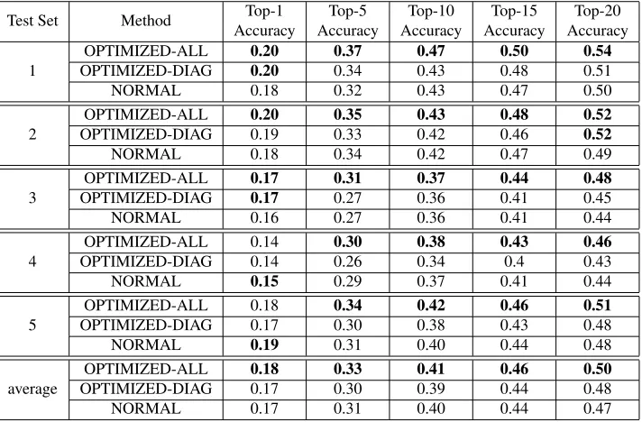
In order to take these random effects into ac-count, we perform repeated subsampling of the standard. In detail, we randomly split the gold-standard into equally-sized training and test set. This is repeated five times, leading to five training and five test sets. The performance on each test set is shown in Table 1. OPTIMIZED-ALL marks the re-sult of our proposed method, where matrixAis opti-mized using the training set. The optimization of the diagonal elementsd1, . . . , d4, and the non-diagonal valuez is as described in Section 4.2. Finally, the baseline method, as described in 3, corresponds to OPTIMIZED-ALL where d1, . . . , d4 are set to 1, andzis set to 0. This baseline is denoted as NOR-MAL. We can see that the overall translation accu-racy varies across the test sets. However, we see that in all test sets our proposed method OPTIMIZED-ALL performs better than the baseline NORMAL.

7_{Note that if the current query (Japanese noun) is a pivot}

word, then the word is not considered as a pivot word.

5.2 Analysis

In the previous section, we showed that the cosine-similarity is sub-optimal for comparing context vec-tors which contain information from different con-text positions. We showed that it is possible to find an approximation of a matrix A which optimally

weights, and combines the different context posi-tions. Recall, that the matrixA is described by the

parametersd1. . . d4andz, which can interpreted as context position weights and a confusion coefficient, respectively. Therefore, by looking at these parame-ters which we learned using each training set, we can get some interesting insights. Table 2 shows theses parameters learned for each training set.

We can see that the parameters, across the train-ing sets, are not as stable as we wish. For example the weight for the predecessor position ranges from 0.27to0.44. As a consequence, the average values,

shown in the last row of Table 2, have to be inter-preted with care. We expect that the variance is due to the limited size of the training set, 220<query, answers>pairs.

Nevertheless, we can draw some conclusions with confidence. For example, we see that the prede-cessor and sucprede-cessor positions are the most impor-tant contexts, since the weights for both are al-ways higher than for the other context positions. Furthermore, we clearly see that the sibling and sentence (bag-of-words) contexts, although not as highly weighted as the former two, can be consid-ered to be relevant, since each has a weight of around 0.20. Finally, we see that z, the confusion

coeffi-cient, is around 0.03, which is small.8 Therefore,

we verify z’s usefulness with another experiment.

We additionally define the method DIAG which uses the same matrix as OPTIMIZED-ALL except that the confusion coefficient z is set

to zero. In Table 1, we can see that the accu-racy of OPTIMIZED-DIAG is constantly lower than OPTIMIZED-ALL.

Furthermore, we are interested in the role of the whole sentence (bag-of-words) information which is in the context vector (in positiond4of the block vec-tor). Therefore, we excluded the sentence

informa-8_{In other words,z is around17%of its maximal possible}

Test Set Method _AccuracyTop-1 _AccuracyTop-5 _AccuracyTop-10 _AccuracyTop-15 _AccuracyTop-20

1

OPTIMIZED-ALL 0.20 0.37 0.47 0.50 0.54 OPTIMIZED-DIAG 0.20 0.34 0.43 0.48 0.51 NORMAL 0.18 0.32 0.43 0.47 0.50

2 OPTIMIZED-DIAGOPTIMIZED-ALL 0.200.19 0.350.33 0.430.42 0.480.46 0.520.52 NORMAL 0.18 0.34 0.42 0.47 0.49

3 OPTIMIZED-DIAGOPTIMIZED-ALL 0.170.17 0.310.27 0.370.36 0.440.41 0.480.45 NORMAL 0.16 0.27 0.36 0.41 0.44

4 OPTIMIZED-DIAGOPTIMIZED-ALL 0.140.14 0.300.26 0.380.34 0.430.4 0.460.43 NORMAL 0.15 0.29 0.37 0.41 0.44

5 OPTIMIZED-DIAGOPTIMIZED-ALL 0.180.17 0.340.30 0.420.38 0.460.43 0.510.48 NORMAL 0.19 0.31 0.40 0.44 0.48

average OPTIMIZED-DIAGOPTIMIZED-ALL 0.180.17 0.330.30 0.410.39 0.460.44 0.500.48 NORMAL 0.17 0.31 0.40 0.44 0.47

Table 1: Shows the accuracy at different ranks for all test sets, and, in the last column, the average over all test sets. The proposed method OPTIMIZED-ALL is compared to the baseline NORMAL. Furthermore, for analysis, the results when optimizing only the diagonal are marked as OPTIMIZED-DIAG.

Training Set d1 d2 d3 d4 z

predecessor successor sibling sentence confusion coefficient

1 0.35 0.26 0.19 0.20 0.03

2 0.27 0.29 0.21 0.23 0.03

3 0.35 0.31 0.16 0.18 0.02

4 0.44 0.24 0.17 0.16 0.04

5 0.39 0.28 0.20 0.13 0.03

average 0.36 0.28 0.19 0.18 0.03

Table 2: Shows the parameters which were learned using each training set. d1. . . d4 are the weights of the context positions, which sum up to1.zmarks the degree to which it is useful to compare context across different positions.

tion from the context vector. The accuracy results, averaged over the same test sets as before, are shown in Table 3. We can see that the accuracies are clearly lower than before (compare to Table 1). This clearly justifies to include additionally sentence information into the context vector. It is also interesting to note that the averagezvalue is now0.14.9 This is consid-erable higher than before, and shows that a bag-of-words model can partly make the use ofzredundant.

However, note that the sentence bag-of-words model covers a broader context, beyond the direct prede-cessors, successor and siblings, which explains why

9_{That is 48% of its maximal possible value. Since for the}

dependency positions predecessor, successor and sibling we get the average weights 0.38, 0.33 and 0.29, respectively.

a smallzvalue is still relevant in the situation where we include sentence bag-of-words into the context vector.

Finally, to see why it can be helpful to compare differentdependency positions from the context vec-tors of Japanese and English, we looked at concrete examples. We found, for example, that the trans-lation accuracy of the query wordディスク_(disc)

improved when using OPTIMIZED-ALL instead of OPTIMIZED-DIAG. The pivot word 歪み (wrap) tends together with both the Japanese query ディ スク_{(disc), and with the correct translation ”disc”}

Method Top-1 Top-5 Top-10 Top-15 Top-20 OPT-DEP 0.13 0.25 0.34 0.38 0.41 NOR-DEP 0.12 0.23 0.29 0.33 0.38

Table 3: The proposed method, but without the sentence information in the context vector, is denoted OPT-DEP. The baseline method, but without the sentence informa-tion in the context vector, is denoted NOR-DEP.

together with the queryディスク_{(disc) in sentences}

like for example the following:

“ブレーキ_(break)ディスク_(disc)に歪み

(wrap)が生じた_(occured)。_”

That Japanese sentence can be literally translated as ”A wrap occured in the brake disc.”, where ”wrap” is the sibling of ”disc” in the dependency tree. How-ever, in English, considered out of the perspective of ”disc”, the pivot word ”wrap” tends to occur in a different dependency position. For example, the fol-lowing sentence can be found in the English corpus:

“Frontdisc wraps.”

In English ”wrap” tends to occur as a successor of ”disc”. A non-zero confusion coefficient allows us to account some degree of similarity to situations where the query (here ”ディスク”(disc)) and the translation candidate (here ”disc”) tend to occur with the same pivot word (here ”wrap”), but in different dependency positions.

6 Conclusions

Finding new translations of single words using com-parable corpora is a promising method, for exam-ple, to assist the creation and extension of bilin-gual dictionaries. The basic idea is to first create context vectors of the query word, and all the can-didate translations, and then, in the second step, to compare these context vectors. Previous work (Laroche and Langlais, 2010; Fung, 1998; Garera et al., 2009) suggests that for this task the cosine-similarity is a good choice to compare context vec-tors. For example, Garera et al. (2009) include the information of various context positions from the dependency-parse tree in one context vector, and, af-terwards, compares these context vectors using the cosine-similarity. However, this makes the implicit

assumption that all context positions are equally im-portant, and, furthermore, that context from differ-entcontext positions does not need to be compared with each other. To overcome these limitations, we suggested to use a generalization of the cosine simi-larity which performs a linear transformation of the context vectors, before applying the cosine similar-ity. The linear transformation can be described by a positive-definite matrixA. We defined the optimal

matrixA by using a Bayesian probabilistic model.

We demonstrated that it is feasible to approximate the optimal matrixAby using MCMC-methods.

Our experimental results suggest that it is bene-ficial to weight context positions individually. For example, we found that predecessor and successor should be stronger weighted than sibling, and sen-tence information. Whereas, the latter two are also important, having a total weight of around 40%. Furthermore, we showed that for languages as dif-ferent as Japanese and English it can be helpful to compare alsodifferentcontext positions across both languages. The proposed method constantly outper-formed the baseline method. Top 1 accuracy in-creased by up to 2% percent points and Top 20 by up to 4% percent points.

For future work, we consider to use different pa-rameterizations of the matrixAwhich could lead to

even higher improvement in accuracy. Furthermore, we consider to include, and weight additional fea-tures like transliteration similarity.

Acknowledgment

We would like to thank the anonymous reviewers for their helpful comments. This work was partially supported by Grant-in-Aid for Specially Promoted Research (MEXT, Japan). The first author is sup-ported by the MEXT Scholarship and by an IBM PhD Scholarship Award.

References

D. Andrade, T. Nasukawa, and J. Tsujii. 2010. Robust measurement and comparison of context similarity for finding translation pairs. In Proceedings of the In-ternational Conference on Computational Linguistics, pages 19–27.

creation. InProceedings of the International Confer-ence on Computational Linguistics and Intelligent Text Processing, Lecture Notes in Computer Science, pages 80–92. Springer Verlag.

S. Basu, M. Bilenko, and R.J. Mooney. 2004. A prob-abilistic framework for semi-supervised clustering. In Proceedings of the ACM SIGKDD International Con-ference on Knowledge Discovery and Data Mining, pages 59–68.

P. Fung. 1998. A statistical view on bilingual lexicon ex-traction: from parallel corpora to non-parallel corpora. Lecture Notes in Computer Science, 1529:1–17. N. Garera, C. Callison-Burch, and D. Yarowsky. 2009.

Improving translation lexicon induction from mono-lingual corpora via dependency contexts and part-of-speech equivalences. In Proceedings of the Confer-ence on Computational Natural Language Learning, pages 129–137. Association for Computational Lin-guistics.

A. Haghighi, P. Liang, T. Berg-Kirkpatrick, and D. Klein. 2008. Learning bilingual lexicons from monolingual corpora. In Proceedings of the Annual Meeting of the Association for Computational Linguistics, pages 771–779. Association for Computational Linguistics. A. Ismail and S. Manandhar. 2010. Bilingual lexicon

extraction from comparable corpora using in-domain terms. InProceedings of the International Conference on Computational Linguistics, pages 481 – 489. A. Laroche and P. Langlais. 2010. Revisiting

context-based projection methods for term-translation spotting in comparable corpora. In Proceedings of the In-ternational Conference on Computational Linguistics, pages 617 – 625.

F. Laws, L. Michelbacher, B. Dorow, C. Scheible, U. Heid, and H. Sch¨utze. 2010. A linguistically grounded graph model for bilingual lexicon extrac-tion. InProceedings of the International Conference on Computational Linguistics, pages 614–622. Inter-national Committee on Computational Linguistics. R. McDonald, K. Crammer, and F. Pereira. 2005. Online

large-margin training of dependency parsers. In Pro-ceedings of the Annual Meeting of the Association for Computational Linguistics, pages 91–98. Association for Computational Linguistics.

N. Okazaki, Y. Tsuruoka, S. Ananiadou, and J. Tsujii. 2008. A discriminative candidate generator for string transformations. InProceedings of the Conference on Empirical Methods in Natural Language Processing, pages 447–456. Association for Computational Lin-guistics.

R. Rapp. 1999. Automatic identification of word transla-tions from unrelated English and German corpora. In Proceedings of the Annual Meeting of the Association

for Computational Linguistics, pages 519–526. Asso-ciation for Computational Linguistics.

Y. Tsuruoka, Y. Tateishi, J. Kim, T. Ohta, J. McNaught, S. Ananiadou, and J. Tsujii. 2005. Developing a ro-bust part-of-speech tagger for biomedical text. Lecture Notes in Computer Science, 3746:382–392.

T. Utsuro, T. Horiuchi, K. Hino, T. Hamamoto, and T. Nakayama. 2003. Effect of cross-language IR in bilingual lexicon acquisition from comparable cor-pora. InProceedings of the conference on European chapter of the Association for Computational Linguis-tics, pages 355–362. Association for Computational Linguistics.