A Tunable Resolution MUSIC Algorithm for Interharmonics Analysis

(1)

http://www.scirp.org/journal/jpee ISSN Online: 2327-5901

ISSN Print: 2327-588X

DOI: 10.4236/jpee.2017.59001 Aug. 31, 2017 1 Journal of Power and Energy Engineering

A Tunable Resolution MUSIC Algorithm for

Interharmonics Analysis

Ming Zhang

1*

_{, Xiang Zhang}

1

_{, Heng Yao}

1

_{, Shunfan He}

2

1_{School of Electronic and Electrical Engineering, Wuhan Textile University, Wuhan, China}

2_{College of Computer Science, South Central University for Nationalities, Wuhan, China}

Abstract

The harmonic and interharmonic analysis recommendations are contained in the latest IEC standards on power quality. Measurement and analysis experiences have shown that great difficulties arise in the interharmonic detection and mea-surement with acceptable levels of accuracy. In order to improve the resolu-tion of spectrum analysis, the tradiresolu-tional method (e.g. discrete Fourier trans-form) is to take more sampling cycles, e.g. 10 sampling cycles corresponding to the spectrum interval of 5 Hz while the fundamental frequency is 50 Hz. How-ever, this method is not suitable to the interharmonic measurement, because the frequencies of interharmonic components are non-integer multiples of the fundamental frequency, which makes the measurement additionally difficult. In this paper, the tunable resolution multiple signal classification (TRMUSIC) algorithm is presented, which the spectrum can be tuned to exhibit high reso-lution in targeted regions. Some simulation examples show that the resoreso-lution for two adjacent frequency components is usually sufficient to measure inter-harmonics in power systems with acceptable computation time. The proposed method is also suited to analyze interharmonics when there exists an undesira-ble asynchronous deviation and additive white noise.

Keywords

Interharmonics Analysis, Tunable Resolution Multiple Signal Classification (TRMUSIC) Algorithm, Subspace Decomposition, Spectral Analysis

1. Introduction

Interharmonics can be thought of as the inter-modulation of the fundamental and harmonic components of the power system with any other frequency com-How to cite this paper: Zhang, M., Zhang,

X., Yao, H. and He, S.F. (2017) A Tunable Resolution MUSIC Algorithm for Interhar-monics Analysis. Journal of Power and Ener-gy Engineering, 5, 1-13.

https://doi.org/10.4236/jpee.2017.59001

Received: July 27, 2017 Accepted: August 28, 2017 Published: August 31, 2017

(2)

DOI: 10.4236/jpee.2017.59001 2 Journal of Power and Energy Engineering

ponents and can be observed in an increasing number of loads. These loads in-clude static frequency converters, cycloconverters, sub-synchronous converter cascades, induction motors, arc furnaces and so on [1].

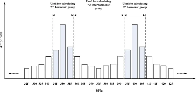
A method, which is aimed to standardize the harmonic and interharmonic measurement, has been proposed by the IEC [2]. This method utilizes discrete Fourier transform (DFT) performed over a rectangular time window of exactly 10 cycles for 50 Hz power systems. The window width fixes the frequency reso-lution at 5 Hz, so the interharmonic components that are between the bins spaced of 5 Hz would spill over primarily into adjacent interharmonic bins with a mini-mum of spill into harmonic bins. Therefore, the harmonic and interharmonic groups are introduced. The interharmonic group is defined as the RMS (Root- mean-square) value of all the interharmonic components between adjacent har-monic groups (seeFigure 1).

However, the accurate estimation method of the interharmonic components has not been established yet. Many researchers have been studying new methods. For analyzing a range of the interharmonic components, researchers often use DFT and its improved algorithms to calculate amplitudes, frequencies and phas-es of the interharmonic components [3][4][5][6][7]. The major pitfalls in the common DFT applications are the spectral leakage and picket fence effects.

The multiple signal classification (MUSIC) algorithm exploits the noise sub-space to estimate the unknown parameters of the random process, which was proposed by R. O., Schmidt [8]. This algorithm can also estimate the frequencies of complex sinusoids corrupted with additive white noise. T. Lobos et al.[9][10] have already proposed the frequencies determination method of the harmonic components using the MUSIC algorithm. But it is difficult to estimate the fre-quencies of the interharmonic components.

[image:2.595.209.539.550.706.2]

In this paper, the tunable resolution MUSIC (TRMUSIC) algorithm is pre-sented to estimate the parameters of interharmonics, which the spectrum can be tuned to exhibit high resolution in targeted regions. The organization of this paper is as follows. The interharmonic measurement method based on the TRMUSIC algorithm is proposed in Section 2. Then, simulation results to demonstrate the

Figure 1. Harmonic and interharmonic (sub) groups.

Amplitude

Used for calculating 7th_{harmonic group}

Used for calculating 7.5 interharmonic

group

Used for calculating 8th_{harmonic group}

350 355 360365 370 375 380385 390 395 400 405 345

340 335 330

325 410 415 420 425

(3)

validity, precision feasibility and robustness of the algorithm are presented in Section 3. At last, the conclusions are given in Section 4.

2. Trmusic Algorithm

2.1. Music Algorithm

The MUSIC algorithm is an eigenvalue subspace decomposition method for es-timation of the frequencies of complex sinusoids observed in additive white noise. Consider a noisy signal vector y comprised of P_{complex sinusoids modeled} as

( )

2π

( )

(

)

1

e i , 0,1, , 1 P

j f n t i i

y n A ∆ e n n N

=

∑

+ =  − (1)

with

eji

i i

A = A ϕ (2)

where Ai , fi and ϕi represent the amplitude, frequency and phase of i-th

complex sinusoid, respectively. N is the number of samples in one data rec-tangular window, ∆t is the fixed time interval, and e n

( )

is a zero mean Gaus-sian white noise vector with variance 2

n

σ .

Suppose that Y

( )

n is the sampled set. Since it is known that

( )

( ) (

)

(

)

T

, 1 , , 1

n =_y n y n+ y n+ −N _

Y  , the Y

( )

n can be expressed as

( )

n =

( ) ( )

f n +

( )

n

Y A X E (3)

with

( )

f = 

( ) ( )

f1 , f2 ,

( )

fP 

A a a ，a (4)

( )

_2π( ) T

1 2π

1, ej fi t, , ej N fi t i

f =  ∆ − ∆_

a  (5)

( )

( ) ( )

( )

T

1 , 2 , , P

n = _x n x n x n _

X  (6)

where

( )

2

ej f ni

i i

x n =A π .

The auto-correlation matrix of the noisy signal Y

( )

n can be written as

( ) ( )

H H 2

E

YY =  n n = XX + EE= +

σ

n

R Y Y R R APA I (7)

where E denotes the expectation, H denotes the Domitian transpose and

( )

H

( )

E n n 

=  

P X X is the diagonal matrix. In addition, H

XX =

R APA and

2

EE =σn

R I are the auto-correlation matrices of the signal and noise processes respectively, as follows

H 1 N XX i i i

i

λυ υ

=

∑

R (8)

2 H 1 N EE n i i

i

σ υ υ

=

∑

R (9)

where λi and υi are the eigenvalues and convector of the matrix RXX,

(4)

H 2 H H

1 1 1

N N N

YY i i i n i i i i i

i i i

λυ υ σ υ υ µ υ υ

= = =

=

∑

+

∑

=

∑

R (10)

where

{

2

}

, 1, 2, ,

i i n i N

µ

= +

λ σ

=  are the eigenvalues of the matrix RYY. All

the eigenvalues are the real numbers and satisfy

2

1 2 p p1 N n

µ

≥

µ

≥≥

µ

>

µ

+ ==

µ

=

σ

(11)

Furthermore, the singular value decomposition (SVD) of the matrix RYY can

be written as

H

YY= Σ

R U V (12)

where the columns of Uand V are the left and right singular vectors, respec-tively. Σ_{is a diagonal matrix whose diagonal entries are the positive}

eigenva-lues of RYY, and Σ =diag

[

µ µ1 2µN

]

.

Then, the MUSIC spectrum is defined as [11]

( )

₂ H

( )

H

( )

H 1 1 1 MUSIC N i i p P f f f f

υ

= + = =

∑

a SS a

a

(13)

with

( )

_2π( ) T

1 2π

1, ej fr t, , ej N fr t r

f =  ∆ − ∆_

a  (14)

[

υP+1 υN

]

=

S  (15)

where a

( )

fr is the complex sinusoidal vector, fr is the frequency resolution of

the MUSIC spectral estimation, and S is the matrix of convector of the noise subspace.

2.2. The Proposed Tunable Resolution Method

The frequency resolution fr of the DFT spectral estimation is low when the

sampling time tc (it is also the width of rectangular window) is short because 1

r c s

f = t = f N, where fs is the sampling frequency. The frequency

resolu-tion can be improved by increasing the number of frequency points, but it may increase the calculation time. The MUSIC algorithm is known as a high-resolution frequency estimation method, however, its frequency resolution fr is

in-variable, which doesn’t allow the best frequency resolution in a dynamic signal. Here, a method of obtaining spectral interpolation data on the use of tunable factor ∆ is presented. According to the required frequency resolution of inter-harmonics analysis, the tunable factor ∆ is decided. Furthermore, the frequency resolution can be adapt adjusted by changing the tunable factor ∆. Thus, a

( )

fr

in Equation (14) can be expressed as

( )

_2π( ) T

1 2π

1, ej fr t, , ej N fr t r

f′ =  ′∆ − ′∆_

a  (16)

with

[

0,1, ,

]

r , r

f

f′ = k ⋅ k= ∆

∆

(5)

where fr′is the frequency bin sets with the tunable factor ∆, fr ∆ is the updated

frequency resolution, and ∆ must be an integer, as shown in Figure 2. There-fore, such data will replace the initial data for the frequencies estimation.

2.3. Denouncing Algorithm Based on Cross-Spectral Estimation

The most important step is to estimate the signal subspace dimension P for spec-tral analysis. However, the noise yields an inconsistent estimation that tends to estimate the number of peaks in the range profile. To overcome this problem a denouncing algorithm based on cross-spectral estimation has proposed.

Assume two signal sequences

( )

( ) (

)

(

)

T

, 1 , , 1

n =_y n y n+ y n+ −N _

Y 

( )

(

)

(

) (

)

(

)

T

, 1 , , 1

n n m y n m y n m y n N m

′ = + =_ + + + + + − _

Y Y 

then

( )

n =

( ) ( )

f n +

( )

n

Y A X E (18)

( )

n

( ) ( )

f n

( )

n

( )

f

( )

n

(

n m

)

′ = ′ + ′ = Ω + +

Y A X E A X E (19)

with Ω =_{diag e}

(

j2πf m t1∆_{, e}j2πf m t2 ∆_,_{, e}j2πf m tP ∆

)

. Thus, the cross-correlation matrix

YY′

R of the noisy signal Y

( )

n and Y′

( )

n is

( )

H

( )

YY′=E n ′ n = XX′+ EE′+ XE′+ EX′

R Y Y R R R R (20)

From Equation (20), the matrix RYY′ is composed of RXX′, which is the

cross-correlation matrix of the clean harmonic signal sequences, REE′, which is

the cross-correlation matrix of the noise sequences, and two other cross-correlation terms RXE′ and REX′. For two noise sequences assumed to be

indepen-dent, we can get REE′ =0 [12]. Typically it is assumed that the clean harmonic

signal and noise sequences are uncorrelated. This has the effect of removing the cross-correlation terms RXE′ and REX′ from the matrix RYY′. Therefore, the

matrix RYY′ simplifies to

( )

H

( )

H H

YY′ =E n ′ n = XX′ = Ω

R Y Y R AP A (21)

where

( )

H

n n

′ = Ω

X X . Equation (21) showsthat the cross-correlation matrix

YY′

R of the noisy signal Y

( )

n and Y′

( )

n is correlative to the noise. Thus, the SVD of the matrix RYY′ can be writtenas [13].

[

]

[

]

H

1 2 1 2

0 0 0 YY′

′ Σ

 

′ ′ ′ ′ ′ ′ ′

= Σ = _ _

 

[image:5.595.244.536.579.714.2]

R U V U U V V (22)

Figure 2. Resolution of MUSIC spectrum.

0 fs/2

Bin Size New Bin Size

nfr

(n-1)fr

(n-2)fr

(6)

where the columns of U′and V′ are the left and right singular vectors respec-tively, and U′=

[

U1′ U2′

]

, V′=

[

V1′ V2′

]

, Σ =′ diag

[

λ λ1, 2,,λP

]

.

In a real application, the cross-correlation matrix RYY′ is not known, and it

should be estimated with sampled data as follows

( ) ( )

( ) (

)

1 1

H H

0 0

1 1

ˆ N N

YY

n n

n n n n m

N N − − ′ = = ′ =

∑

=

∑

+

R Y Y Y Y (23)

The matrix RYY′ also takes the form

11 12 1

21 22

1 2 ˆ

N

YY

N N NN

r r r

r r

R

r r r

′       =              (24)

where each elementrij

(

i j, =1, 2,,N

)

is a positive real number such that

(

) (

)

1 0 1 N ij n

r y n i y n j

N

−

=

′

=

∑

+ ⋅ + .

So, the Equation (23) can be used to estimate the signal subspace dimension P accurately. For example, because zero coefficients are concentrated in the higher-lags, a noise robust algorithm by using only the lower-lags of the matrix

ˆ YY′

R can be designed to estimate the signal subspace dimension P. Therefore, Equation (13) can be rewritten as

( )

2 H

( )

H

( )

H 1 1 1 MUSIC N i i P P f f f f υ = + = = ′ ′ ′

∑

a S S a

a

(25)

where S′ is the updated matrix of convector of the noise subspace.

2.4. Estimation Method of the Amplitude and Phase of the

Harmonic and Interharmonic Components

The frequencies of the harmonic and interharmonic components can be esti-mated from the peak location of the MUSIC spectrum, i.e., the frequencies

{

fi,i=1, 2,,p

}

can be derived from the horizontal coordinate of the peak

point of PMUSIC

( )

f . After the estimation of the frequencies, the signal subspace

dimension P of the input signal can also be estimated. In a real application,

( )

ˆ

y n is not known. Because the amplitude of the noise is very smaller than that of the signal components, let y n

( )

replaces y nˆ

( )

. Then, the estimation

( )

ˆ

y n of y n

( )

can be represented by

( )

( ) ( )

2π

1

ˆ e i

P j f n t

i i

y n y n e n ∆ A

=

= − =

∑

⋅ (26)

where n=0,1,,

(

N−1

)

. , i.e.,

( ) ( ) ( )

( )

(

)

1 2

1 1 1

1

2π 2π 2π

2

2π 1 2π 1 2π 1

ˆ 0

1 1 1

e e e ˆ 1

ˆ

e e e 1

P j f t j f t j f t

j f N t j f N t j f N t P

y A

A y

A y N

(7)

Equation (27) can be used to solve least squares for the coefficients

{

A ii, =1, 2,,p

}

using only the available data samples [14]. Therefore, the

amplitude and phase of the components can be obtained from

{

A ii, =1, 2,,p

}

, as follows

( )

(

)

2

(

( )

)

2

Re Im

i i i

A = A + A (28)

( )

Im arctan

Re i i

i

A

ϕ = _ _

  (29)

where Re( )⋅ returns the real part of the argument, and Im( )⋅ returns the

im-aginary part of the argument.

3. Simulation Results

Three cases are performed in Matlab to demonstrate the effectiveness of the pro-posed algorithm.

3.1. Case 1

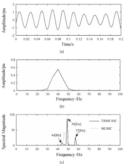
In practice, the fundamental frequency often deviates from its nominal value. In the first simulation, the fundamental frequency is set to 49 Hz, and the signal is

( )

0.1sin 2

(

π44 30

)

sin 2

(

π49 45

)

0.2 2

(

π57 60

)

( )

y t = t+  + t−  + t+  +e t (30)

the sampling frequency fs is 6400 Hz, the number of samples N is 1280 (10

cycles), the noise variance 2 n

σ _{is 0.1, the tunable factor} ∆ is set to 5. It can be seen from Equation (30) that includes the interharmonic components of 44 Hz and 57 Hz. Figure 3 displays the spectrums of MUSIC algorithm based on auto- spectral estimation, TRMUSIC algorithm based on cross-spectral estimation, and DFT algorithm when the width of rectangular window is 0.2 s (10 cycles), respectively.

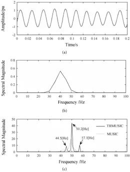
In the second simulation, the fundamental frequencies is set to 50.2 Hz, and the signal is

( )

0.1sin 2π44.5 30

(

)

sin 2π50.2 45

(

)

0.2 2π57.3 60

(

)

( )

y t = t+  + t−  + t+  +e t (31)

the sampling frequency fs is 6400 Hz, the number of samples N is 1280, the

noise variance 2 n

σ _{is 0.1, the tunable factor} ∆ is set to 50. It can be seen from Equation (31) that includes the interharmonic components of 44.5 Hz and 57.3 Hz. Figure 4 displays the spectrums of the MUSIC algorithm based on auto- spectral estimation, TRMUSIC algorithm based on cross-spectral estimation, and DFT algorithm when the width of rectangular window is 0.2 s, respectively.

(8)

(a)

(b)

[image:8.595.245.503.67.403.2]

(c)

Figure 3. Spectrums of DFT, MUSIC and TRMUSIC algorithm for the first simulation: (a) Original signal; (b) DFT spectrum; (c) MUSIC and TRMUSIC spectrum.

the tunable factor ∆ is set to 50, the frequency resolution of the TRMUSIC al-gorithm is 0.1 Hz. It is seen from Figure 4 that the TRMUSIC spectrum has sharp peaks. Figure 4 shows the accurate frequencies estimation of the funda-mental and interharmonic components (44.5 Hz, 50.2 Hz, 57.3 Hz).The corres-ponding estimation results are listed in Table 1.

3.2. Case 2

(9)

(a)

(b)

[image:9.595.243.504.72.417.2]

(c)

Figure 4. Spectrums of DFT, MUSIC and TRMUSIC algorithm for the second simulation: (a) Original signal; (b) DFT spectrum; (c) MUSIC and TRMUSIC spectrum.

Table 1. Results of fundamental and interharmonic components measurement.

Case

Frequency [Hz] Amplitude [Pu] Phase [degree]

True Values

TRMUSIC Estimation Values

True Values

1

44 44 0.1 0.099 30 30.7237

49 49 1 1.001 −45 −44.8523

57 57 0.2 0.199 60 60.6537

2

44.5 44.5 0.1 0.098 30 30.6235

50.2 50.2 1 1.002 −45 −44.7641

57.3 57.3 0.2 0.1998 60 60.5574

[image:9.595.208.540.493.653.2]

(10)

(a) (b)

[image:10.595.61.539.69.525.2]

(c) (d)

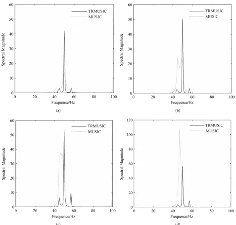
Figure 5. Comparison between the auto-spectral and cross-spectral estimation algorithm: (a) Simulation 1; (b) Simulation 2; (c) Simulation 3; (d) Simulation 4.

3.3. Case 3

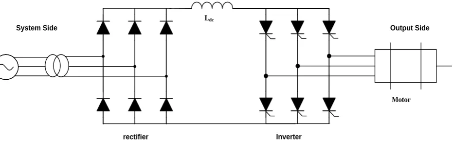
This simulation analyzes the harmonics in the AC/DC/AC converter system. The AC/DC/AC converter system is a typical source of interharmonics [7] [15]. The inter-harmonic frequencies of the input current derive from the mod-ulation of the converter harmonic components of operated by the rectifier har-monics (see Figure 6). The simulation model of the AC/DC/AC converter sys-tem is established in Matlab/Simulation. The parameters of the model are as fol-lows. The parameters of the ac supply are Us =25 3 KV,Ls=1 H,Rs=20Ω.

The inductance of the dc side is Ldc =5mH. The parameters of load are 50 H

l

(11)

[image:11.595.69.535.73.219.2]

Figure 6. AC/DC/AC converter system.

Y-Y connection. The fundamental frequencies of system side and output side are 50 Hz and 60 Hz, respectively.

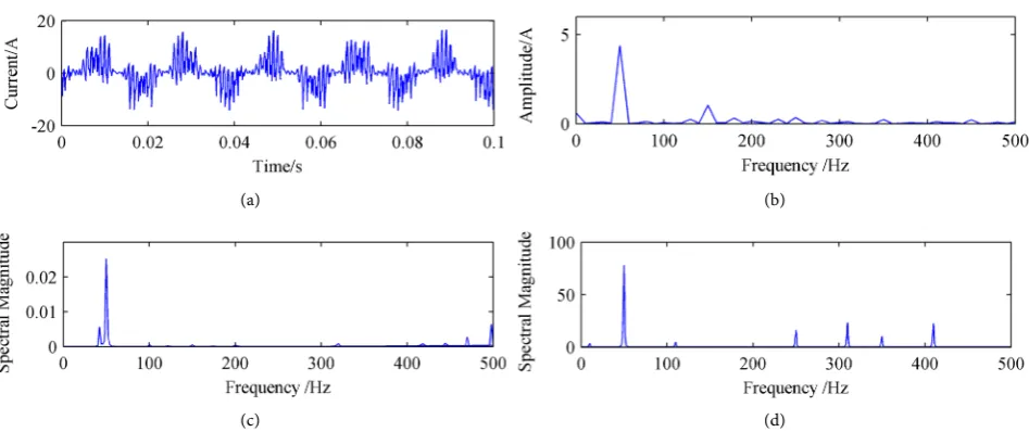
Figure 7 shows the interharmonics analysis results of current wave of phase B of the supply system side (5 cycles of samples). The components in the signal are measured by the TRMUSIC algorithm, which the tunable factor ∆ is set to 10. The frequencies of characteristic harmonics in system side are

(

6k±1

)

fm

( )

fm

is the fundamental frequency of system side). It can be seen from Figure 7 that the system side of 50 - 60 Hz AC/DC/AC converter system includes not only the characteristic harmonics of 50 Hz, 250 Hz, and 350 Hz, but also the interhar-monics of 10 Hz, 110 Hz, 310 Hz, and 410 Hz, although the amplitudes of some interharmonics are small.

Then, the results of the TRMUSIC algorithm are compared with that of the MUSIC and DFT algorithm. For this simulation, we can see that the frequency analysis precision of the TRMUSIC algorithm is higher than that of the MUSIC and DFT algorithm, because the frequency resolution of the MUSIC and DFT algorithm is 10 Hz while that of TRMUSIC algorithm is 1 Hz, respectively. In Figure 7, when the frequencies don’t locate closest to the value of the integer frequency, the estimations with the TRMUSIC algorithm are quite accurate by predetermining the proper tunable factor ∆. Unfortunately, this may result in false frequency components with the MUSIC and DFT algorithm, and it requires a longer data record. From the simulation, it is shown that the TRMUSIC algorithm indeed has a clearly higher frequency analysis precision than the MUSIC and DFT algorithm.

3.4. Comparison with MUSIC and DFT Algorithm

If fast Fourier transform (FFT) algorithm is used to compute its DFT, one such limitation is the power-of-two rule, requiring the number of input samples to be an integer power of two (i.e., 128, 256, 512). Therefore, choosing to lower sam-pling frequencies for better resolution is no longer a viable option. A clever en-gineer would simply increase the number of samples being taken. However, this solution quickly gets out of hand. In spite of this, the TRMUSIC algorithm may never be faster than the DFT algorithm.

Ldc

Inverter rectifier

System Side Output Side

(12)

(a) (b)

[image:12.595.64.538.70.269.2]

(c) (d)

Figure 7. Interharmonics analysis of 50 - 60 Hz AC/DC/AC converter system: (a) Current wave of phase B in system side; (b) DFT spectrum; (c) MUSIC spectrum; (d) TRMUSIC spectrum.

Compared to the traditional MUSIC algorithm, the TRMUSIC algorithm is much more flexible. Given the required frequency resolution of interharmonic analysis, you can choose the proper tunable factor ∆_{. Having expended the}

fort on increasing the accuracy, the TRMUSIC algorithm can be carried out ef-fectively.

4. Conclusions

This paper proposes an effective method to estimate the parameters of inter-harmonics in power systems. With the increase of points in time domain, the frequency resolution is improved because the frequency resolution of MUSIC algorithm is fs N while that of TRMUSIC algorithm is fs

(

∆ ⋅N

)

. Moreover,

the frequency resolution of TRMUSIC algorithm can be adapt adjusted by chang-ing the tunable factor ∆.

This research is very fundamental as an application to interharmonic analysis. Many tests were made in this work and the TRMUSIC algorithm is the most suitable to be used when estimating interharmonic spectrum. It gives us a handy solution for some drawbacks that can be found in methods like the DFT or tra-ditional MUSIC algorithm.

The TRMUSIC algorithm really meets the need of offline applications. Fur-thermore, if this algorithm can be implemented in parallel computation, it should meet the need of online applications and be more practical.

Acknowledgements

This work is supported by National Natural Science Foundation of China (No. 51477124).

References

(13)

Con-DOI: 10.4236/jpee.2017.59001 13 Journal of Power and Energy Engineering

trol in Electric Power Systems. IEEE, New York.

[2] IEC (2002) General Guide on Harmonics and Interharmonics Measurements and

Instrumentation for Power Supply Systems and Equipment Connected Thereto. IEC, Geneva.

[3] Edison, B. and Alpine, M. (2016) An Evaluation of the Extent of Correlation

be-tween Inter-Harmonic and Voltage Fluctuation Measurements. IEEE Transactions

on Power Delivery, 31, 753-760. https://doi.org/10.1109/TPWRD.2015.2480715

[4] Lin, H.C. (2016) Identification of Interharmonics Using Disperse Energy

Distribu-tion Algorithm for Flicker Troubleshooting. IET Science, Measurement &

Tech-nology, 10, 786-794. https://doi.org/10.1049/iet-smt.2016.0110

[5] Sun, Z., He, Z., Bang, T. and Li, Y. (2016) Multi-Interharmonic Spectrum

Separa-tion and Measurement under Asynchronous Sampling CondiSepara-tion. IEEE

Transac-tions on Instrumentation and Measurement, 65, 1902-1912.

https://doi.org/10.1109/TIM.2016.2562278

[6] Chen, C. and Chen, Y. (2014) Comparative Study of Harmonic and Interharmonic

Estimation Methods for Stationary and Time-Varying Signals. IEEE Transactions

on Industrial Electronics, 61, 397-404. https://doi.org/10.1109/TIE.2013.2242419

[7] Hui, J., Yang, H., Bu, W. and Li, Y. (2012) A Method to Improve the Interharmonic

Grouping Scheme Adopted by IEC Standard 61000-4-7. IEEE Transactions on

Power Delivery, 27, 971-979. https://doi.org/10.1109/TPWRD.2012.2183394

[8] Schmidt, R.O. (1986) Multiple Emitter Location and Signal Parameter Estimation.

IEEE Transactions on Antennas and Propagation, 34, 276-280.

https://doi.org/10.1109/TAP.1986.1143830

[9] Lobos, T., Napoleonic, Z., Reamer, J. and Schemer, P. (2000) High-Resolution

Spectrum-Estimation Methods for Signal Analysis in Power Systems. IEEE

Transac-tions on Instrumentation and Measurement, 55, 219-225.

https://doi.org/10.1109/TIM.2005.862015

[10] Leonowicz, Z., Lobos, T. and Rezmer, J. (2003) Advanced Spectrum Estimation

Methods for Signal Analysis in Power Electronics. IEEE Transactions on Industrial

Electronics, 50, 514-519. https://doi.org/10.1109/TIE.2003.812361

[11] Kaveh, M. and Barabell, A.J. (1986) The Statistical Performance of the MUSIC and

the Minimum-Norm Algorithms in Resolving Plane Waves in Noise. IEEE

Transac-tions on Acoustics, Speech and Signal Processing, 34, 331-341.

https://doi.org/10.1109/TASSP.1986.1164815

[12] Pisarenko, V. (1973) The Retrieval of Harmonics from a Covariance Function.

Geo-physical Journal of the Royal Astronomical Society, 33, 347-366.

https://doi.org/10.1111/j.1365-246X.1973.tb03424.x

[13] Gu, J.F. and Wei, P. (2007) Joint SVD of Two Cross-Correlation Matrices to

Achieve Automatic Pairing in 2-DAngle Estimation Problems. IEEE Antennas &

Wireless Propagation Letters, 6, 553-556.

https://doi.org/10.1109/LAWP.2007.907913

[14] Hasan, M.K., Fattah, S.A. and Khan, M.R. (2003) Identification of Noisy AR

Sys-tems Using Damped Sinusoidal Model of Auto-Correlation Function. IEEE Signal

Processing Letters, 10, 157-160. https://doi.org/10.1109/LSP.2003.811590

[15] Li, C., Xu, W. and Tayjasanant, T. (2003) Interharmonics: Basic Concepts and

Techniques for Their Detection and Measurement. Electric Power Systems

(14)

Submit or recommend next manuscript to SCIRP and we will provide best service for you:

Accepting pre-submission inquiries through Email, Facebook, LinkedIn, Twitter, etc. A wide selection of journals (inclusive of 9 subjects, more than 200 journals)

Providing 24-hour high-quality service User-friendly online submission system Fair and swift peer-review system

Efficient typesetting and proofreading procedure

Display of the result of downloads and visits, as well as the number of cited articles Maximum dissemination of your research work

Submit your manuscript at: http://papersubmission.scirp.org/