Predictive ability of three different estimates of “cay” to excess stock returns A comparative study Germany & U S

Predictive ability of three different

estimates of “cay” to excess stock returns

A comparative study Germany U.S

-Emara, Noha

Rutgers University

2014

Online at

https://mpra.ub.uni-muenchen.de/68686/

Predictive Ability of Three Different Estimates of “cay”

To Excess Stock Returns

- A Comparative Study Germany & U.S -

Noha Emara Assistant Professor Economics Department Rutgers University 311 Armitage Hall N. 5th Street, room 313 Camden, NJ 08102

http://economics.camden.rutgers.edu/emara.html cell: (201) 920 4510

office: (856) 225-6096

Abstract

Outline

Introduction………..3

Section I.Three ways of estimating the Trend Relationship Among Consumption, Labor Income and Asset Holdings……….3

Section II - Asset Return Data and the correlation matrix………...5

Section III- Quarterly In-Sample Forecasting Regressions……….6

Section IV. Out-of-Sample Nested forecasting regression………8

Section V. Out-of-Sample Non-Nested forecasting regression………...10

Section VI- Conclusion………..12

Introduction

Over long horizons financial variables like the ratios of price to dividends, price to earnings or dividends to earnings had predictive power for excess returns over a treasury-bill rate. However, stock returns have typically found to be only weakly forecast able. Moreover, traditional macroeconomic variables like consumption, assets and labor income have proven to have stronger predictive power for excess returns over treasury-bill rate.

Lettau and Ludvigson (2001) have shown the trend deviations of these macroeconomic variables is a strong predictor of the of the excess stock returns over a treasury bill rate, and can account for a substantial fraction of the variation in future excess returns. Where the variable that reflects these deviations is called “cay”.

In this paper we will compare three different ways of estimating this trend deviation in Germany and U.S over the period 1969:2 to 2005:1. The variables will be called “cay-Ols”, “cay-Dls” and “cay-LL”. Where the first refers to estimating the macroeconomic trend deviations using the ordinary least square method, the second refers to estimating it by the dynamic least square method and finally the third variable refers to estimation by the Ludvigson and Lettau method.

The ability of these three variables, cay-Ols , cay-Dls and cay-LL, besides other tradional variables like dividend ratio, pay-out ratio and bill rate to predict in-sample excess stock return over treasury bill rate in both Germany an U.S will be compared. In addition the out-of sample forecast of cay-Ols, cay-Dls and cay-LL using fixed estimation scheme for the period 1990:1 to 2005:1 will also be estimated. The mean squared error MSE-F test will be used to test for the ability of the unrestricted model (the one includes the variable cay) to hold all the information contained by the restricted model or “encompass”. The out-of sample forecast of alternative non-nested models will also be compared. The Diebold Mariano (1995) test will be used to test for the equivalence accuracy of the two models under comparison.

The paper is organized as follows; Section I explains three ways of estimating the trend relationship among consumption, labor Income and asset Holdings. Section II explains the asset return data and the correlation matrix; section III quarterly in-sample forecasting regressions; Section IV Out-of-Sample Nested forecasting regression; Section VOut-of-Sample Non-Nested forecasting regression; Section VI concludes and section VII references.

I- Three ways of estimating the Trend Relationship Among Consumption, Labor Income and Asset Holdings;

weighted deutsche mark and 2000 chain weighted dollars for Germany and U.S respectively. The data for the stock market capitalization and demand deposits in Germany and U.S were used as a proxy for asset wealth. Finally the data for gross national income was used as a proxy for labor income. All the data for Germany and U.S have been collected from the data bases of the “Global Finance” and “International Financial Statistics” As a preliminary step, the variables are tested whether each variable passes a unit root test. It has been found that consumption, labor income and assets for both countries contain a unit root.

In (Lettau, M.; Ludvison, S.,(2001)) they showed that cay_t can be a good proxy for market expectations of future asset returns as long as expected future returns on human capital and consumption growth are not too volatile, or as long as these variables are highly correlated with expected returns on assets. All the terms on the right –hand side of equation (1) are presumed stationary, c, a, and y must be cointegrated, and the left side of (1) gives the deviation in the common trend of c_t,a_t,y_t. This trend deviation term

t t

t a y

c −ω −(1−ω) will be denoted as cay_t.

t i t i t h i t a i i t t t

t a y E r r c z

c (1 ) {[ _, (1 ) _, ] } (1 )

1 ω ω ω ρ ω

ω − − = _ω + − −Δ + −

− + + +

∞

=

∑

(1) In this study we will present three different ways of estimating this trend deviation. A description of the estimation is as follows;

Method 1: dynamic least squares (DLS) technique

The first method used to estimate the term cay is the DLS. This method specifies a single equation taking the following form has been followed;

∑

∑

− = − − − = + Δ + Δ + + + = k k i t i t t y i t k k i i a t y t a t

n a y b a b y

c , α β β , , ε (2)

where Δ denotes the first difference operator.

This method generates optimal estimates of the cointegrating parameters a multivariate setting. The DLS specification adds leads and lags of the first difference to the right-hand side variables to a standard OLS regression of consumption on labor income and asset holdings to eliminate the effects of the regressor endogeneity on the distribution of the least square estimator. The estimated trend deviation will be taken as the residual of equation (2) and will be denoted as “Cay-DLS”.

Method 2: Ordinary Least Square (OLS) Technique

The second method of estimating the trend deviations is the OLS. In this method Equation (2) will be estimated with only the lags of asset wealth and labor income included. Cay is then considered to be the residual of the significant regression. The Cay under this second method will be denoted as “Cay-OLS”.

Method 3: Ludvigson ,M. and Lettau, S. (2001) Technique

least square technique as in equation (2), the taking the coefficients of asset wealth and labor income of the significant regression1 , Cay is then calculated as follows;

(3) The estimated cay under this method will be denoted as “Cay-LL”.

The point estimates for the parameters of consumption, labor income and assets for Germany is ;

c_n,t =−0.008+0.0234a_t +0.551yt (2) (-0.63) (5.968) (34.1)

While the point estimates for the equivilant model for the U.S is;

c_n,t =−3.628+0.015a_t +01.150yt (3) (-7.3) (3.5) (37.18)

where the corrected t-statistics appear in parentheses below the coefficient estimates.

II - Asset Return Data and the correlation matrix:

The financial quarterly data for both Germany and U.S include stock index, dividends yield, pay-out ratio and bill rate. Denoting “ER” is the quarterly excess return, “DIV” is the log dividends yield, “p/e” is the quarterly pay-out ratio, “Br” as the quarterly bill rate and finally the terms “Cay-Ols”, “Cay-Dls” and “Cay-LL” are defined previously before.

Table I Correlation Matrix

Panel A: Germany

t

ER DIV_t P_t /e_t

t

Br _{Cay LL}

t − cayt−Ols cayt −Dls

t

ER 1 0.12 0.13 -0.072 0.18 0.11 0.09

t

DIV 1 0.17 0.013 0.08 0.08 0.07

t t e

P/ 1 0.07 0.07 0.01 0.02

t

Br 1 0.12 0.11 0.10

Cay-LL 1 0.91 0.92

Cay-Ols 1 0.98

Cay-Dls 1

Panel B: U.S

t

ER 1 -0.81 0.85 0.68 0.40 0.43 0.38

t

DIV 1 -0.90 -0.71 0.01 0.01 0.02

t t e

P/ 1 0.66 0.21 0.21 0.20

t

Br 1 0.15 0.12 0.12

LL

Cay_t − 1 0.96 0.95

Ols

cay_t− 1 0.95

Dls

cay_t − 1

1 _{The significant regression was chosen based on the AIC measure.} t

y t a t

n a y

c y

The above table shows the correlation matrix between the financial quarterly data including the three different estimates of ‘cay”. Panel A shows the correlation matrix in Germany, while panel B shows the corresponding values in the U.S. As for the sake of our analysis, we will concentrate on the last three columns of the table. As it can be noticed from this table, the positive and between the three estimates of caˆy and the excess return ERt for both Germany and U.S . However the correlation estimates for the

U.S are much higher for the three different methods of caˆy, which are in turn less than the correlation coefficients of the p/e and Br for the U.S. On the other hand, the correlation with the dividend yield is negative and big for the U.S too.

An important point to notice about this table is the correlation coefficients between the three different estimates of cay. As can be noticed these correlations exceeds the ninety percent for the two countries. The correlation between cay-Dls and cay-Ols is the highest for Germany, while the correlation between cay-LL and cay-Ols is the highest for the U.S.

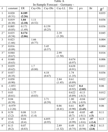
III- Quarterly In-Sample Forecasting Regressions

In this section, the forecasting power of different variables for the quarterly excess stock returnERt will be estimated. Table A in the appendix reports estimates from

OLS regressions of excess stock returnsERt on lagged variables named at the head of the

columns for Germany, and table B in the appendix reports the equivalent estimates of the U.S.

From regression 1 to 2 or 2’ or 2’’, it can be noticed that including any of the measures of “cay” has improved the significance of the whole model, however from line 2’ we can notice that including cay-LL has the greatest impact on improving the significance of the model over the other two measures of cay. This result is confirmed when comparing lines 3, 3’ and 3’’. However from regression lines 5, 5’ and 5’’, the Cay-Dls proved to have the greatest impact on the in-sample forecasting ability of the whole model. This result is confirmed from lines 7, 7’ and 7’’. Finally, adding all the financial indicator of our model, the models where Cay-Dls and Cay-LL proved to have almost the same ability to improve the significance of the model which is little less than the model that includes Cay-Ols. What is surprising about the in-Sample results is that the parameters of the three estimates of “cay’ are not significant, however the signs are as theoretically expected . These results are in accordance with the economic intuition of the expectation of returns. If returns are expected to decline in the future, investors who desire smooth consumption paths will allow consumption to dip temporarily below its long-term relationship with both assets and labor income in an attempt to insulate future consumption from lower returns, and vice versa (Lettau, M.; Ludvison, S.,(2001)). Thus investors’ own optimizing behavior suggest that deviations in the long-term trend among c, a, y should be positively related to future stock return, consistent with the results of the table above.

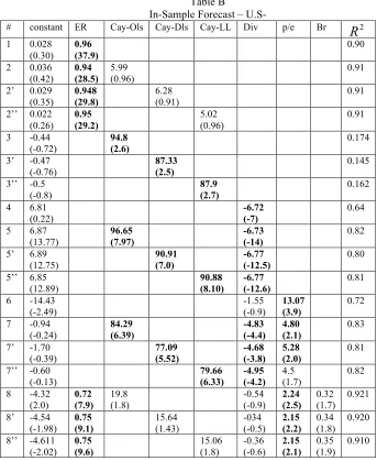
From the in-sample forecast of the U.S we can notice the following; adding the different estimates of “cay’ to our model of line 1 had slightly improved the significance of the model, as obvious from lines 2, 2’ and 2’’. Though including the three different cay’s had almost the same 2

From regression lines 3, 3’ and 3’’ we can notice that cay-Ols has the highest _R2.

This result is confirmed from lines 5, 5’ and 5’’when the dividends yield are added to the model, and confirmed again from lines 7, 7’ and 7’’ when the pay-out ratio is added to the model and again from lines 8, 8’ and 8’’ when all the variables have been added all together. As can be noticed from table B, and opposite to table A, that all the parameters of the different cay’s are significant at the five percent level of significance. The significant parameters are highlighted in bold numbers. In addition, the signs of the parameters are as expected by economic theory.

IV. Out-of-Sample Nested forecasting regression

From the in-sample forecast of excess return, especially the case of Germany, we were not able to get significant estimates for almost all the parameters. Specifically, the three different estimates of cay were not significant in providing in-sample forecast of excess stock return over the treasury-bill return. To eliminate the bias that might be due to the fact that these estimates of “cay” were estimated using the coefficient of the whole sample. In this section, the data will be split into two subsamples, the insample period will start from the second quarter of 1969 to the fourth quarter of 1989. We then use fixed estimation scheme to re-estimate the model for the period from the first quarter of 1990 to the first quarter of 2005.

We begin by making nested forecast comparisons. We compare the mean-squared forecasting error from an unrestricted model, which includes any of the three estimates of “cay’, to a restricted benchmark model, which excludes this variable. Thus the unrestricted model nests the benchmark model.

Table C in the appendix provides nested forecast comparisons where two bench marks are used alternatively . The first part of the table compares two nested model in turn, the restricted model contains the constant expected returns as the explanatory variable while the unrestricted model contains any of the different estimates of cay besides the constant term. The second part of the table we use another benchmark which is the random walk. The comparison provided in the following table is the mean squared errors from the restricted model and the different unrestricted models. It can be noticed for the case of Germany that the mean squared errors of the nested out-of-sample forecast of the three different estimates of cay are higher than the constant bench mark model. However the mean squared errors of the unrestricted model that includes Cay-Ols or Cay-Dls are lower than the mean squared error of the random walk benchmark model.

On the other hand, for the case of U.S the unrestricted Cay-Ols model proved to have the lower mean squared error in the constant bench mark model, while the Cay-Dls proved to have the lower mean squared error in the random walk bench mark.

alternative is that the restricted model has a higher MSE. The test statistic are compared with the tabulated values provided by ( McCracken(1999)) for the fixed scheme2.

The F-test is calculated as follows;

c u L P u L P P T R t t T R t t ˆ ) ˆ ( ) ˆ

( 1 _{2, 1}

1 , 1 1 _⎟ ⎠ ⎞ ⎜ ⎝ ⎛ − ⎟ ⎠ ⎞ ⎜ ⎝ ⎛

∑

∑

= + − = + − (4)

where

∑

= + − = T R t t u P c 1 , 2 1 _ˆ

ˆ and uˆi_,t+₁ =L(uˆi_,t+₁) i=1,2. where 1 refers to the restricted model

and 2 refers to the unrestricted model.

TableII

Mean Squared Error F-Test

U.S Germany Row Comparison MSE_u /MSE_{r Statistic} MSE MSE

u/ Statistic

1 Cay-Ols vs. constant 0.99 0.00072* 1.8 28.59 2 Cay-Dls vs. constant 1.005 0.0284* 1.6 25.47 3 Cay-LL vs. constant 1.001 0.0366* 3.9 47.02 4 Cay-Ols vs. random walk 1.01 1.0097** 0.97 1.54*** 5 Cay-Dls vs. random walk 1.11 6.684 0.97 1.72*** 6 Cay- LL vs. random walk 0.92 5.19 1.7 26.6

*significant at the ten percent. ** significant at the ten percent. *** significant at the ten percent.

Calculating the test statistic for the six comparisons for both the Germany and the U.S, we can notice that for the U.S, Cay-Ols is the only significant nested model either when the benchmark model is the constant or the random walk. This result confirm what has been found for the significance Cay-Ols in the in-Sample forecast section. Both the nested models that includes either Cay-Dls or Cay-LL are significant only when the constant benchmark model is used for comparison.

On the other hand, for the case of Germany, we are still unable to find any significant out-of-sample forecast for excess returns by the nested models that includes Cay-Ols, Cay-Dls or Cay-LL when the constant benchmark model is used. These results are already been confirmed for the in-sample forecast. However, both Ols and Cay-Dls provide a significant out-of –sample forecast when the random walk excess return is used as the bench mark model.

V. Out-of-Sample Non-Nested forecasting regression

In this section we compare a set of nonnested forecast comparisons in which the lagged value of the three different techniques of estimating “cay” is the sole predictive variable are alternately compared with competitor models in which either the lagged excess return, lagged dividend yield, lagged payout ratio, or lagged bill rate is the sole predictive variable.

In this section the Diebold Mariano test will be used. The Diebold Mariano (DM) test is an out-of-sample test for equal predictive accuracy of two non nested model. The DM test simply assumes “no parameter estimation error” or that the out-of-sample period grows less quickly than the in-sample period. In addition the DM test assumes that the two models are non-nested.

The null under DM test is as follows;

Diebold Mariano (1995) shows that under the null hypothesis of equal predictive ability, has an asymptotically standard normal distribution.

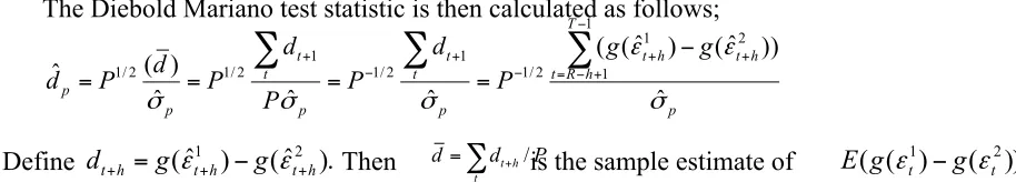
The Diebold Mariano test statistic is then calculated as follows;

Define Then is the sample estimate of

[image:10.612.89.546.241.323.2]

The calculated test statistic is then compared to the t-table, accordingly we were able to reject the null hypothesis of equal predictive accuracy between the three estimates of cay and alternative variables.

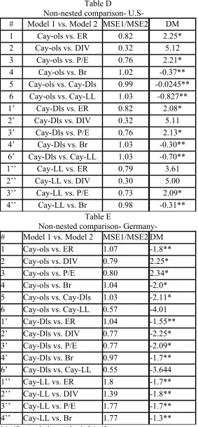
Table D in the appendix reports the test statistic of the results of the Diebold Mariano test statistic for the out-of-sample forecast of non-nested models. At the five percent level of significance we reject the null hypothesis of equal predictive power of almost all models except for model comparisons number 4, 5, 6, 4’, 6’ and 4’’. In other words, the results shows that there is equal predictive ability of the different methods of estimating “cay” to estimate excess return in U.S. What was not expected is that we cannot reject the hypothesis of equal predictive ability of the different types of cay and the bill rate. We can also notice that the three different methods of estimating cay do not have equal predictive accuracy when compared to the dividend yield, as shown in line 2, 2’ and 2’’.

From table E in the appendix, at the five percent level of significance, we reject almost all the models of equal predictive accuracy. What is important to be noted from the results of the following table is that we cannot accept the hypothesis of equal predictive accuracy between the three different methods of estimating “cay’ and this result is different from what has been found for the case of U.S, where the equivalent accuracy prediction of the three methods of estimating “cay” has been proved.

VI- Conclusion

The results of (Lettau, M.; Ludvison, S.,(2001)) show that Cay-LL has a significant predictive power both in the in-sample and the out-of-sample forecast of excess return. Our study departs from Lettau, M.; Ludvison, S.,(2001) in adding and

0 )) ( ) ( (

: 1 2

0 E g t −g t =

H ε ε

0 )) ( ) ( (

: _t1 − _t2 ≠

A E g g

H ε ε

p T h R t h t h t p t t p t t p p g g P d P P d P d P d σ ε ε σ σ σ ˆ )) ˆ ( ) ˆ ( ( ˆ ˆ ˆ ) ( ˆ 1 1 2 1 2 / 1 1 2 / 1 1 2 / 1 2 /

1

∑

∑

∑

− + − = + + − + − + − = = = = ). ˆ ( ) ˆ

( t1h t2h h

t g g

d+ = ε+ − ε +

P d d t h t /

∑

+

= _{( (} 1_{) (} 2_)).

t t g g

comparing other two estimates of “cay” namely Ols’ and Dls” besides “Cay-LL” in forecasting excess return in both Germany and U.S over the period 1969:2 to 2005:1.

Our results show that for the case of U.S, “Cay-Ols” has a better in-sample forecasting ability over the other two estimates of cay. Also, our results prove that Cay-Ols has displayed statistically significant out-of sample predictive power of excess return, and contains information that is not included in the lagged value of excess return. In addition, a model of constant expected returns is rejected in favor of a model of a time varying expected returns when Cay-Ols is used as the predictive variable. The Cay-Dls and Cay-LL have also improved the in-sample forecast of excess return but they are not as powerful as Cay-Ols. In addition, according to our results, Cay-Dls and Cay-LL were not robust in the Sample forecast of excess return in U.S. The results of the out-of-sample forecast of the non-nested model show that the mean squared forecast error is lower when Cay-LL is used as a predictive variable than when any other predictive variable is employed. However checking for the statistical significance of the results, Cay-ols, Cay-Dls and Cay-LL proved to have equal predictive accuracy.

Our results also show that for the case of Germany, the three estimates of “cay” are neither significant in the in-sample forecast of excess return, nor is any of these estimates contain information that is not included in the constant expected returns model. however, checking for the out-of –sample predictive accuracy of nested models, Cay-Ols and Cay-Dls has displayed statistically significant out-of-sample predictive power for excess return and contains information that is not included in lagged value of the excess return. Cay-LL on the other hand, has proved not to hold any extra information for predicting excess returns as compared to a model of lagged expected excess returns or constant excess returns. Parallel to these findings, the out-of-sample forecast of the non-nested models shows that Cay-Ols and Cay-Dls do not have equal predictive accuracy as compared to Cay-LL.

VII- Reference:

Campbell,John Y. “A Variance Decomposition for Stock Returns.” Econ. J (march 1991): 157-79.

---, ” Understanding Risk and Return.” J.P.E 104 (April 1996): 298-345.

Campbell, John Y., and Cochrane, John H.,’ By Force of Habit: A consumption Based Explanation od Aggregate Stock Market Behavior.” J.P.E 107 (April 1999): 205-51.

Campbell, John Y., and Shiller, Robert J. “The Dividend-Price Ratio and Expectations of Future Dividends and Discount Factors” Rev. Financial Studies: 195-228.

Clark, Todd and Michael McCracken, 1999, Tests of Equal Forecast Accuracy and encompassing for nested models, Working paper, Federal Reseve Bank of Kansas City.

Harvey, David, Stephen Leybourne, and Paul Newbold, 1998, Tests for Forecast ecvompassing, Journal of Business and Economic statistics 16,254-259.

Lettau, Martin, and Ludvigson, Sydney. “Consumption, Aggregate Wealth, and Expected Stock Returns.” J. Finance 56 (June 2001): 815-49.

Michael W. McCracken, 1999, Asymptotics for out of Sample Tests of Causality’,

[image:13.612.135.480.116.539.2]

Appendix

Table A In-Sample Forecast – Germany -

# constant ER Cay-Ols Cay-Dls Cay-LL Div p/e Br 2

R

1 0.020

(0.31)

0.189 (2.26)

0.035

2 0.019

(0.30) 1.84 (2.18) 1.11 (0.52) 0.036

2’ 0.005 (0.05) 0.171 (1.49) 0.159 (0.25) 0.036

2’’ 0.035 (0.54) 0.174 (2.06) 2.39 (1.20) 0.045

3 0.023

(1.66)

1.66 (0.77)

0.004

3’ 0.016 (0.09)

3.45 (0.57)

0.004

3’’ 0.044 (0.67)

2.99 (1.50)

0.016

4 0.040

(0.63)

0.674 (0.97)

0.006

5 0.039

(0.62) 1.7 (0.80) 0.638 (0.91) 0.011

5’ 0.037 (0.35) 4.18 (0.67) 1.74 (1.35) 0.036

5’’ 0.058 (0.90) 2.84 (1.45) 0.61 (0.89) 0.022

6 -1.053 (-2.68) 0.627 (0.92) 0.4 (2.82) 0.06

7 0.03

(0.61) 1.77 (0.83) 0.622 (0.89) -0.13 (-0.3) 0.012

7’ 0.04 (0.39) 3.71 (0.59) 1.80 (1.39) -0.84 (-0.9) 0.047

7’’ -0.979 (-2.26) 0.86 (0.41) 0.61 (0.90) 0.37 (2.43) 0.06

8 0.59

(3.2) 0.08 (0.9) 3.13 (1.4) 0.48 (0.7) -0.05 (-0.1) -43 (-3) 0.11

8’ 0.83 (2.4) 0.04 (0.4) 6.055 (0.95) 1.25 (0.99) -0.56 (-0.6) -57 (-2.4) 0.13

[image:14.612.135.478.88.507.2]

Table B

In-Sample Forecast –

U.S-# constant ER Cay-Ols Cay-Dls Cay-LL Div p/e Br 2

R

1 0.028

(0.30)

0.96 (37.9)

0.90

2 0.036

(0.42) 0.94 (28.5) 5.99 (0.96) 0.91

2’ 0.029 (0.35) 0.948 (29.8) 6.28 (0.91) 0.91

2’’ 0.022 (0.26) 0.95 (29.2) 5.02 (0.96) 0.91

3 -0.44

(-0.72)

94.8 (2.6)

0.174

3’ -0.47 (-0.76)

87.33 (2.5)

0.145

3’’ -0.5 (-0.8)

87.9 (2.7)

0.162

4 6.81

(0.22)

-6.72 (-7)

0.64

5 6.87

(13.77) 96.65 (7.97) -6.73 (-14) 0.82

5’ 6.89 (12.75) 90.91 (7.0) -6.77 (-12.5) 0.80

5’’ 6.85 (12.89) 90.88 (8.10) -6.77 (-12.6) 0.81

6 -14.43 (-2.49) -1.55 (-0.9) 13.07 (3.9) 0.72

7 -0.94

(-0.24) 84.29 (6.39) -4.83 (-4.4) 4.80 (2.1) 0.83

7’ -1.70 (-0.39) 77.09 (5.52) -4.68 (-3.8) 5.28 (2.0) 0.81

7’’ -0.60 (-0.13) 79.66 (6.33) -4.95 (-4.2) 4.5 (1.7) 0.82

8 -4.32

(2.0) 0.72 (7.9) 19.8 (1.8) -0.54 (-0.9) 2.24 (2.5) 0.32 (1.7) 0.921

8’ -4.54 (-1.98) 0.75 (9.1) 15.64 (1.43) -034 (-0.5) 2.15 (2.2) 0.34 (1.8) 0.920

8’’ -4.611 (-2.02) 0.75 (9.6) 15.06 (1.8) -0.36 (-0.6) 2.15 (2.1) 0.35 (1.9) 0.910 Table C Mean Squared Errors Benchmark Unrestricted models

Constant Cay-Ols Cay-Dls Cay-LL Germany 0.1481 0.267849 0.24618 0.558 U.S 0.213771 0.213769 0.214725 0.213894

Table D

Non-nested comparison-

U.S-# Model 1 vs. Model 2 MSE1/MSE2 DM 1 Cay-ols vs. ER 0.82 2.25* 2 Cay-ols vs. DIV 0.32 5.12 3 Cay-ols vs. P/E 0.76 2.21* 4 Cay-ols vs. Br 1.02 -0.37** 5 Cay-ols vs. Cay-Dls 0.99 -0.0245** 6 Cay-ols vs. Cay-LL 1.03 -0.827** 1’ Cay-Dls vs. ER 0.82 2.08* 2’ Cay-Dls vs. DIV 0.32 5.11 3’ Cay-Dls vs. P/E 0.76 2.13* 4’ Cay-Dls vs. Br 1.03 -0.30** 6’ Cay-Dls vs. Cay-LL 1.03 -0.70** 1’’ Cay-LL vs. ER 0.79 3.61 2’’ Cay-LL vs. DIV 0.30 5.00 3’’ Cay-LL vs. P/E 0.73 2.09* 4’’ Cay-LL vs. Br 0.98 -0.31**

Table E

Non-nested comparison- Germany- # Model 1 vs. Model 2 MSE1/MSE2 DM 1 Cay-ols vs. ER 1.07 -1.8** 2 Cay-ols vs. DIV 0.79 2.25* 3 Cay-ols vs. P/E 0.80 2.34* 4 Cay-ols vs. Br 1.04 -2.0* 5 Cay-ols vs. Cay-Dls 1.03 -2.11* 6 Cay-ols vs. Cay-LL 0.57 -4.01 1’ Cay-Dls vs. ER 1.04 -1.55** 2’ Cay-Dls vs. DIV 0.77 -2.25* 3’ Cay-Dls vs. P/E 0.77 -2.09* 4’ Cay-Dls vs. Br 0.97 -1.7** 6’ Cay-Dls vs. Cay-LL 0.55 -3.644 1’’ Cay-LL vs. ER 1.8 -1.7** 2’’ Cay-LL vs. DIV 1.39 -1.8** 3’’ Cay-LL vs. P/E 1.77 -1.7** 4’’ Cay-LL vs. Br 1.77 -1.3**

[image:15.612.166.449.88.698.2]