Microblog Emotion Classification
by Computing Similarity in Text, Time, and Space
Anja SummaDepartment of Computational Linguistics
Heidelberg University Heidelberg, Germany
Bernd Resch Department of Geoinformatics – Z GIS
University of Salzburg Salzburg, Austria
Michael Strube NLP Group Heidelberg Institute for Theoretical Studies gGmbH
Heidelberg, Germany
Abstract
Most work in NLP analysing microblogs focuses on textual content thus neglecting temporal and spatial information. We present a new interdisciplinary method for emotion classification that combines linguistic, temporal, and spatial information into a single metric. We create a graph of labeled and unlabeled tweets that encodes the relations between neighboring tweets with respect to their emotion labels. Graph-based semi-supervised learning labels all tweets with an emotion. 1 Introduction and Motivation
Social media analysis is a field where natural language processing (NLP) and geographic information science (GIScience) overlap, because messages posted in social media frequently contain both textual and geographical information. While GIScience researchers have adopted NLP methods to analyze the textual layer of tweets, spatio-temporal analysis is virtually non-existent in NLP (very recently Volkova et al. (2016) distinguished emotions across very coarse geolocations). Steiger et al. (2015) state that only 4% of the publications dealing with spatio-temporal Twitter analysis come from computational linguistics. By merely analysing the tweets’ text, temporal and spatial information is lost. Also, in most cases NLP and GIScience methods are not directly combined, but used as two different processing steps. One example is sentiment analysis on geo-referenced Twitter data (Bertrand et al., 2013). Here sentiment is computed purely semantically, and its results are interpreted according to the tweets’ spatial and temporal layers.
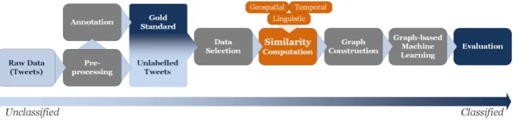
[image:1.595.113.491.609.697.2]The work presented here aims to overcome this desideratum by applying GIScience methods in an NLP context. The overall workflow is shown in Figure 1. The textual and spatio-temporal dimensions of tweets are jointly used by one comprehensive graph-based semi-supervised machine learning method to label tweets with their prevalent emotions. This setup has the benefits of being applicable to both GIScience and NLP as well as needing only a small amount of labeled data. To create a gold standard, we manually label a subset of our Twitter data with a set of emotion classes. To keep the task feasible, This work is licensed under a Creative Commons Attribution 4.0 International Licence. Licence details: http: //creativecommons.org/licenses/by/4.0/
Figure 1: Workflow: In Step 1, a set of tweets is preprocessed and partly annotated in order to construct a gold standard. Those data are used for experiments. A subset is selected and in Step 3 used to construct a graph via similarity computing. In Step 4, a graph-based semi-supervised machine learning algorithm classifies emotions. In Step 5, evaluation is performed.
Portland St. and Main. on scene. #mitshooting
This is awful RT: BREAKING: MIT officer has died from his injuries. #7NEWS I’m at Central Square (Cambridge, MA) w/2others
That just pissed me off
-Table 1: Tweets from dataset dealing with events around Boston Marathon Bombing
we agree on a subset of Ekman’s basic emotions (Ekman and Friesen, 1971), as defined by Jack et al. (2014): HAPPINESS,FEAR,SADNESS, andANGER/DISGUST(merged in one category, see Section 3.2). Additionally, we utilize aNONEclass to catch all other cases.
In this paper, we focus on computing the similarity between two nodes, i.e. tweets, which is used to construct the graph (Figure 1). The similarity score is utilized as edge weight. On the resulting graph we apply Modified Adsorption (Talukdar and Crammer, 2009), a semi-supervised label-propagation al-gorithm. Features are derived from and extend work on Twitter sentiment analysis and Twitter writing style analysis such as work on authorship attribution on microblogs (Schwartz et al., 2013).
We choose the time and geolocation around the Boston Marathon Bombing because we expect to harvest a larger fraction of highly emotional tweets than usual. See Table 1 for a few examples from our dataset some of which express emotions. The GIScience aspects of this work are described in detail in a companion paper (Resch et al., 2016).
2 Related Work
Emotion recognition can be viewed as a subtask of sentiment analysis (Liu and Zhang, 2012). It is, how-ever, more complex as it addresses multiple emotions, and, hence, requires a multi-class classification (Kozareva et al., 2007), instead of the binary or gradual polarity categories used mostly in sentiment analysis. Sentiment analysis on Twitter data has attracted a lot of research (Strapparava and Mihalcea, 2008; Davidov et al., 2010; Bollen et al., 2011; Roberts et al., 2012; Pak and Paroubek, 2010; Brody and Diakopoulos, 2011; Kouloumpis et al., 2011) with, e.g., several years of shared tasks at SemEval and more than 30 participating teams at the SemEval 2016 Task 4. Still, the results are still far from perfect and quite a bit worse than results on reviews (Nakov et al., 2016).
Existing work classifying emotions in tweets is supervised and requires large amounts of annotated data (Roberts et al., 2012; Mohammad and Kiritchenko, 2014; Volkova and Bachrach, 2016) or heuristics deriving emotions from hashtags to label emotions in tweets (Davidov et al., 2010). We, in contrast, apply a semi-supervised method which requires only little annotated data. While Bollen et al. (2011) label discrete emotions, they do not classify single tweets but examine the whole Twitter community jointly. Roberts et al. (2012) and Bollen et al. (2011) use the temporal dimension, but neglect the spatial dimension (georeferencing of single tweets had been introduced only in 20091).
There is only little work in NLP dealing with geolocation in tweets. Han et al. (2014), Rahimi et al. (2015b) and Rahimi et al. (2015a) use tweets to predict geolocation, the reverse of our setting. However, Rahimi et al. (2015a) use a model based on Modified Adsorption which is relatively close to our model. Volkova et al. (2016) use a very coarse notion of geolocation and find differences in emotions across different countries. Bertrand et al. (2013) use geolocation in tweets to perform sentiment analysis. They base their work onThe First Law of Geography: “everything is related to everything else, but near things are more related than distant things” (Tobler, 1970, p.4). We also follow this law.
Our semi-supervised approach is based on the idea that similar tweets should be labeled with similar emotions. However, approaches for computing “Semantic Textual Similarity” (Agirre et al., 2012) are not applicable as emotions are not expressed that much through content words but through the text’s linguistic and stylistic properties. Hence, our features are closer to ones used in linguistic style analysis as used in, e.g., work on authorship attribution on tweets (Layton et al., 2010; Silva et al., 2011; Macleod and Grant, 2012; Schwartz et al., 2013). Linguistic style analysis also has been applied to sentiment analysis in tweets (Pak and Paroubek, 2010; Kouloumpis et al., 2011; Brody and Diakopoulos, 2011).
everybody hates you
Does this state a fact? Is this written by someone feeling sorry someone else? Does this show anger/disgust/hate? Can I knock out right here?
Sounds and looks emotional, but what exactly does it mean? haha
Is that happiness? Or meant ironically and really encodes sadness?
Table 2: Tweets causing arguments among annotators. Tweet text and remarks made during discussion.
3 Data and Annotation
Existing datasets comprising short texts and emotion annotations (Strapparava and Mihalcea, 2007; Roberts et al., 2012; Volkova and Bachrach, 2016) can not be used for our purposes as they do not contain spatio-temporal information. The dataset by Volkova et al. (2016) contains spatio-temporal in-formation, but the work is done on Ukranian and Russian. Hence, we create our own dataset.
3.1 Raw Data
In order to increase the likelihood that the tweets contain emotions, we collect tweets from the Boston area in the two weeks around the Boston Marathon Bombing on April 15th, 2103. Raw data is provided by the Center for Geographic Analysis at Harvard University which collects tweets using a public Twitter REST Geo Search API (https://dev.twitter.com/rest/public) via spatial search queries (Harvard University, Center for Geographic Analysis, 2016). This provides us withall georeferenced tweets from a particular area instead of just a sample as would have been the case if the Streaming API would have been used with spatial information (Boyd and Crawford, 2012). We select tweets from April 8th, 2013 to April 22nd, 2013, georeferenced within a bounding box containing Boston with: xmin: -71.21, ymin: 42.29, xmax: -70.95, ymax: 42.25. Preprocessing comprises language detection by two language detectors (McCandless, 2010; Lui and Baldwin, 2012) so that only tweets are kept which are identified by at least one detector as English, removing tweets without content (i.e., tweets being empty after filtering URLs and @mentions). After preprocessing 195,380 georeferenced tweets remain.
3.2 Emotion Annotation
We choose Ekman’s six basic emotionshappiness, anger, sadness, disgust, surprise, and fear (Ekman and Friesen, 1971) plusnoneas a basis for our annotation. These categories have been used in related work (Strapparava and Mihalcea, 2008; Roberts et al., 2012; Purver and Battersby, 2012).
We train seven naive (neither experts in psychology nor in NLP) subjects to annotate tweets and to perform an initial reliability study. It turns out that two annotators are not up to the task (after computing pairwiseκ(Fleiss, 1971) between annotators). So we continue with five annotators who annotated 261 randomly selected tweets. Also, theκscores fordisgustandsurpriseare very low. See Table 2 for a few examples which caused arguments among annotators during the first phase of the annotation.
Hence we change the annotation manual so that the likely to be confused emotionsangeranddisgust
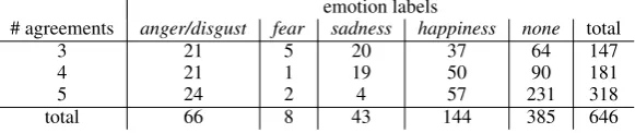
are merged, andsurpriseis annotated asnone. This leads to the satisfyingκscores reported in Table 3. After having refined the annotation scheme and after having established a pool of five annotators, we proceed with randomly selecting another 385 tweets which are annotated by all five annotators. We merge both sets of annotations to create a gold standard for our experiments. We follow M¨uller (2007) in creating several gold standard levels based on the number of annotations agreeing with each other. This way a gold standard with sufficient quality can be produced albeit at the cost of losing some annotations (Table 4). none is the most frequent class followed by happiness. We originally expected a higher fraction of tweets encodinganger/disgust,fearandsadness, but our two week window proved to be too long. For our experiments we combine gold standard levels 4 and 5 which gives us 499 annotated tweets.
emotion labels
# agreements anger/disgust fear sadness happiness none total
3 21 5 20 37 64 147
4 21 1 19 50 90 181
5 24 2 4 57 231 318
[image:4.595.153.444.64.125.2]total 66 8 43 144 385 646
Table 4: Number of gold standard labels per emotion class and agreement level
4 Computing Similarity between Tweets
In graph-based semi-supervised learning the edge weights encode the degree of influence between neigh-boring nodes. For emotion classification on tweets, this means that two nodes connected by a strong edge are likely to receive the same emotion label. We define the edge weight in a way that supports this re-lation:Similarityisthe likelihood that two tweets contain the same emotion. This relation is defined to be symmetric for each pair of tweets, which results in an undirected graph. If a tweet receives overall similarity scores of 0 to all other tweets in the data set, it is not part of the graph and thus cannot be la-beled. Computing this similarity, we leverage the special nature of tweets. Thus, similarity is computed along the dimensionstext (Section 4.1),time, and geographic space(Section 4.2). After intermediate results for all dimensions are computed individually, they are combined into one score (Section 4.3).
This concept of similarity is different from others in mainly three ways: (1) It does not require semantic analysis, because the tweets’ topic is not of interest. (2) It does not work on vector representations. (3) To our best knowledge, it is the first similarity measure that combines the three dimensions text, time and geo-space. We do not use vectors because they cannot be applied in our graph-based semi-supervised learning setting.
4.1 Linguistic Similarity
The textual dimension is computed by analysing the tweet’s writing style. We assume that a similar writing style encodes a similar emotion2. This approach is inspired by work on Twitter sentiment analysis
(Pak and Paroubek, 2010; Brody and Diakopoulos, 2011; Kouloumpis et al., 2011). Twitter authorship analysis (Layton et al., 2010; Macleod and Grant, 2012; Schwartz et al., 2013; Silva et al., 2011) also provides insight into writing style analysis. Research in both fields shows that although tweets are short, unedited text, writing style analysis provides information about the user and her emotions.
Linguistic similarity between tweets is computed as follows: First, two tweets are analyzed and com-pared with respect to specific linguistic aspects (Section 4.1.1). Second, these similarities are normalized and aggregated and alinguistic similarity scoreis returned (Section 4.1.2).
4.1.1 Feature Design
The feature design is influenced by the transductive setting inherent to Modified Adsorption, which means that there are no separate training and labeling phases and thus no model is built. Consequently, only properties that can be (1) extracted from a single tweet or (2) computed from comparing two tweets are suitable features. This excludes any approaches that require an analysis of the corpus as a whole, such as language models per category or word frequencies. The features are designed to be mostly language independent. The only language-specific resource applied is ANEW3(Bradley and Lang, 2010).
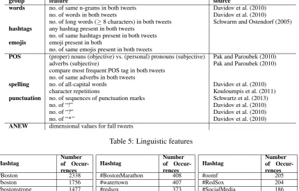
The features we apply can be divided into two major groups (see Table 5): those that compare con-crete words and those that analyze generic style characteristics. In order to facilitate experimenting the individual features are organized into feature groups depending on the examined grammatical entity.
2The termsimilar emotionis applicable in this case, because the granularity of the emotion model applied here is low. Thus, while two tweets may be rightly classified into the same emotion class, they may in reality express different variants of abasic emotion(cf., e.g. Shaver et al. (1987)).
group feature source
words no. of same n-grams in both tweets Davidov et al. (2010) no. of words in both tweets Davidov et al. (2010)
no. of long words (≥8 characters) in both tweets Schwarm and Ostendorf (2005)
hashtags any hashtag present in both tweets no. of same hashtags present in both tweets
emojis emoji present in both
no. of same emojis present in both tweets
POS (proper) nouns (objective) vs. (personal) pronouns (subjective) Pak and Paroubek (2010)
adverbs (subjective) Pak and Paroubek (2010)
compare most frequent POS tag in both tweets no. of same adverbs in both tweets
spelling no. of all-capital words Davidov et al. (2010)
character repetitions Kouloumpis et al. (2011)
punctuation no. of sequences of punctuation marks Schwartz et al. (2013)
no. of “!” Davidov et al. (2010)
no. of “?” Davidov et al. (2010)
no. of “"” Davidov et al. (2010)
[image:5.595.81.512.66.341.2]ANEW dimensional values for full tweets
Table 5: Linguistic features
Hashtag Numberof Occur-rences #Boston 2338 #boston 1756 #bostonstrong 1477 #Job 1399 #BostonStrong 1063 #Jobs 944 #bostonmarathon 731 #TweetMyJobs 672 #Marketing 591 #prayforboston 490
Hashtag Numberof Occur-rences #BostonMarathon 408 #watertown 407 #redsox 373 #internship 335 #tmlt 319 #TeamFollowBack 263 #jobs 257 #Follow2BeFollowed 219 #Watertown 219 #Cambridge 206
Hashtag Numberof Occur-rences #oomf 205 #RedSox 204 #SocialMedia 186 #manhunt 179 #advertising 174 #marathonmonday 167 #love 163 #spring 150 #fenway 150 #2 130
Table 6: 30 most frequent hashtags in the data set.
String Features. We use words, hashtags, and emojis returned by Owoputi et al. (2013)’s POS tagger. We compare n-grams of different sizes, the overall number of words and the overall number of long words (≥8 characters) in the two tweets. Tweets are characterized by the microblog-specific entitieshashtags
(Chang, 2010) andemojiswhose distribution may also indicate their emotional content. Table 6 lists the 30 most frequent hashtags in our data. Some hashtags have emotional content (e.g. #bostonstrong, #prayforboston). Davidov et al. (2010) regard hashtags and emojis as sentiment assigned by the user. Kouloumpis et al. (2011) use hashtags to acquire a training set of positive, negative, and neutral tweets. We also use hashtags as a feature to compute the similarity between tweets. Emojis have an even stronger emotional content than hashtags. Hence, we use them for the same purpose.
Style Features. POS tagsdo not directly convey emotion information, but their distribution within a text has been shown to reveal a text’s polarity (Pak and Paroubek, 2010). However, the POS tagger used (Owoputi et al., 2013) does not tag adjectives correctly. Hence we can only use adverbs in our feature set. Spelling featurestake spelling pecularities as intensifiers(Eisenstein, 2013; Kouloumpis et al., 2011): the number of words containingcharacter repetitionsand the number of words writtenin only capital letters. We takepunctuationas an encoding of emotional content (as suggested by Davidov et al. (2010)). We compare exclamation, question, and quotation marks as sequences and as counts.
4.1.2 Normalising and Aggregating Results
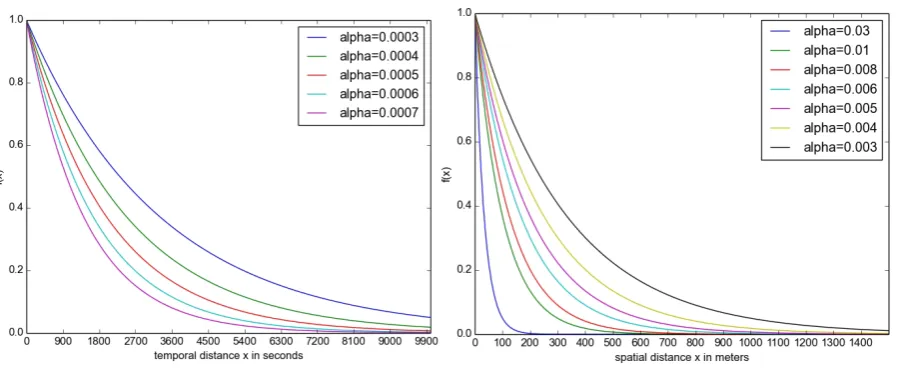
Figure 2: Temporal (left) and spatial similarity (right): Differentαvalues for comparison.
sim(Ta, Tb) =ζ×simling(Ta, Tb) +β×simspat(Ta, Tb) +γ×simtemp(Ta, Tb) (1)
4.2 Temporal and Spatial Similarity
Extracting spatio-temporal information from microblogs requires methods from GIScience. Twitter can be regarded as “a new type of a distributed sensor system”, allowing for insights into spatio-temporal processes by generating a “geographic footprint” (Crooks et al., 2013, p.2). Using this concept of hu-man sensors, people offer subjective observations of their environment as opposed to technical sensors creating reproducible measurements. We utilize the concept ofTwitter users as geo-sensorsbecause it allows to interpret tweets as observations and to relate those observations temporally and spatially to the environment. Even though no complete model of the spatio-temporal dynamics of Twitter has been suggested so far, previous research has operated under the assumption that Waldo Tobler’sFirst Law of Geographyalso holds true for tweets: “everything is related to everything else, but near things are more related than distant things” (Tobler, 1970, p.4).
Bertrand et al. (2013) show that people tweet differently during the course of a day or a week and prove that different places are characterized by latent sentiment. This indicates a causal connection between a person’s location and their mood. Also, the overlapping influences of temporal and spatial patterns have to be considered. Natural disasters have been shown to create a large amount of immediate georeferenced local responses on Twitter (Crooks et al., 2013), but also a longer-lasting world-wide echo (Lee et al., 2011). Crooks et al. (2013, p.2) note that “people frequently comment on events happening at or affecting their location, or refer to locations that represent momentary social hotspots”.
Although there possibly is a connection between a tweet and its origin in time and space, it is not clear how to quantify it. Thus, we suggest a different method: Instead of modeling certain events’ influence on the Twitter stream, we model for two tweets how likely they have been generated by the same event. Sakaki et al. (2010) successfully model the temporal distribution of tweets commenting on a certain event as an exponential function. We apply this approach for both the temporal and spatial layers using f(x) = e(−α×x). Figure 2 shows the relation between two tweets depending on their temporal/spatial distance and adecay parameterα. We suggest those values based on the assumption that two tweets are most likely to have been triggered by the same event if they are close in time and space. In order to favor those tweets that have been written in reaction to something the user has seen with her own eyes, we set reference frames that contain the major part of the curves in Figure 2.
4.3 Combining The Three Dimensions
The similarity scores for all dimensions are combined linearly (Equation 1; simling(Ta, Tb) denotes
micro-average macro-average
features P R F P R F
ling. hashtags 0.6388 0.6388 0.6388 0.1277 0.2 0.1559 punctuation 0.6388 0.6388 0.6388 0.1277 0.2 0.1559 spelling 0.6388 0.6388 0.6388 0.1277 0.2 0.1559 ANEW 0.6412 0.631 0.636 0.1282 0.1975 0.1555 emojis 0.6825 0.6825 0.6825 0.2729 0.2506 0.2613
POS 0.6388 0.6388 0.6388 0.1277 0.2 0.1559
words 0.6388 0.6388 0.6388 0.1277 0.2 0.1559 emojis, hashtags 0.6825 0.6825 0.6825 0.2729 0.2506 0.2613 emojis, punctuation 0.6825 0.6825 0.6825 0.2729 0.2506 0.2613 emojis, spelling 0.6825 0.6825 0.6825 0.2729 0.2506 0.2613 emojis, ANEW 0.6858 0.6151 0.6485 0.1372 0.1925 0.1602 emojis, POS 0.68 0.6746 0.6773 0.2665 0.2432 0.2543 emojis, words 0.6967 0.6746 0.6855 0.3222 0.2432 0.2772 comb. emojis, temporal 0.6388 0.6388 0.6388 0.1277 0.2 0.1559
comb. emojis, spatial 0.6825 0.6825 0.6825 0.2729 0.2506 0.2613
comb. emojis, spat., temp. 0.6825 0.6825 0.6825 0.2729 0.2506 0.2613
random baseline 0.2137 0.2566 0.2332
[image:7.595.129.468.62.264.2]majority baseline 0.6388 0.6388 0.6388
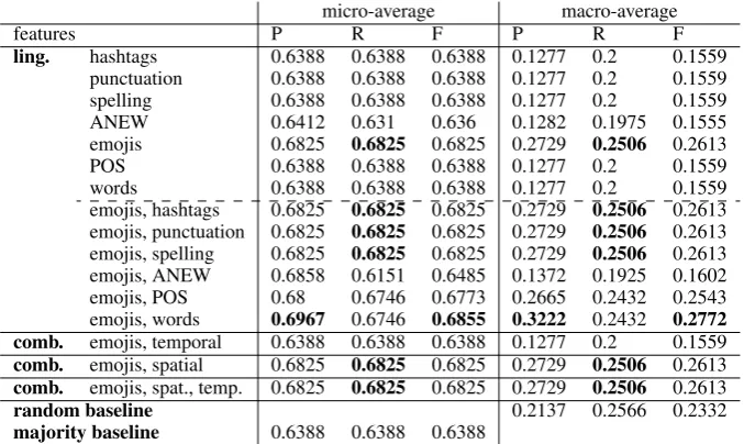
Table 7: Results using Modified Adsorption, agreement level 4, minimum edge weight 0.5
Im a pretty girl. Find me ;) cause we always talk about you :)
awww lmao homie ok :) I don’t mind you making fun of me either haha .. Had a great time at Lauren’s art reception today. My friends have such talent :-)
Table 8: Tweets correctly labeled with happiness
weighting parametersζ, β, andγ. An additional parameter influences the resulting graph’s layout. To exclude noisy edges that do not carry information but bloat the graph, we apply anedge weight threshold. Consequently, only edges whose weight is equal to or higher than this threshold are included in the graph.
5 Experiments
For the experiments we use the gold standard constructed in Section 3 divided into 50% seed data for the semi-supervised graph-based machine learning algorithm and 50% testing data. Graph construction is guided by the similarity computation method described in Section 4. Classification is performed by Modified Adsorption, the semi-supervised label propagation algorithm implemented in theJunto-toolkit4
(Talukdar and Crammer, 2009).
From the gold standard we use level 4, i.e. all tweets which have been annotated with the same label by at least four out of five annotators. This way we make use of more than 75% of the annotated data while ensuring high quality annotations for learning and evaluation. In addition we use 10,000 unlabeled tweets for learning. We set the threshold for edges (minimum weight) to 0.5.
In Table 7 we report the results in terms of micro- and macro-average precision, recall and F-measure. Since the classes have a skewed distribution, results for micro- and macro-average show a large differ-ence. We apply McNemar’s test to report statistically significant differences (Dietterich, 1998). Random and majority decisions serve as baselines for comparison. The macro-average results should be compared with the random baseline, the micro-average results with the majority baseline.
Most of the linguistic features taken on its own perform just like the majority class classification, i.e., they classify each tweet asnone. OnlyANEW andemojismanage to classify some tweets differently. WithANEW this leads to a slight decrease in performance, withemojisto an improvement (statistically significant improvement in recall). A closer inspection of the results shows that both features pick up on the second largest class and label some tweets correctly withhappiness. See Table 8 for some tweets correctly labeled with happiness in the final setting.
When combining the strongest linguistic featureemojiswith other lingustic features,ANEWandPOS
lead to slight decrease in performance while combining emojisandwords achieves the best results in F-measure which is due to a higher precision. Adding further linguistic features does not cause any improvement.
Temporal and spatial features on their own do not classify anything correctly. When combiningemojis
with temporal features (with a range of different values forα) we observe a drop in performance. When combining with spatial features and with spatial and temporal features, there is no difference to just emo-jis. Further experiments with temporal and spatial features show that they lead to a small but statistically not significant improvement when weighted much higher than linguistic similarity (e.g.×5). Highest values forαperformed best (i.e. lowest curves in Figure 2).
6 Discussion
Our research allows an interesting glance into the way emotions are displayed in microblogs: While we expected prevalent emotions to be negative because of the terrorist attack that took place during the time span we examined, Table 4 shows that the opposite is true. Table 6 provides a possible explanation for this: hashtags such as #bostonstrong can mask negative feelings. We evaluate our method using micro- and macro-averaged precision, recall, and F-measure (Tsoumakas et al., 2010). Experiments show that we can recognizenone andhappinessbetter than suitable baselines. The overall best-performing feature group wasemojis. Our analysis of tweets revealed that negative emotions frequently cause tweets conveying a positive emotion. This leads to a skewed seed distribution (Table 4), and hence infrequent labels are rarely assigned at all. This phenomenon requires further research. Random selection of seed tweets may not have been such a good idea, because only very few of our seeds are temporally or spatially close enough. Further experiments should check whether a tighter spatial and temporal distribution of the seed tweets would enable the temporal and spatial features to have a positive impact. For now we have to conclude that linguistic features are superior to temporal and spatial features for Twitter emotion classification. Future research should define improved linguistic features and search for optimal temporal/spatial parameter settings.
Acknowledgments. We acknowledge the German Research Foundation (DFG) for supporting the project “Urban Emotions”, reference numbers ZE 1018/1-1 and RE 3612/1-1. We would like to thank Dr. Wendy Guan from Harvard University’s Center for Geographic Analysis for her support through providing us with Twitter data. We would like to thank G¨unther Sagl, Enrico Steiger, Ren´e Westerholt, Clemens Jacobs and Sebastian D¨oring for supporting the annotation procedure. We would like to thank the Doctoral College GIScience (DK W 1237-N23) at the Department of Geoinformatics–Z GIS, Uni-versity of Salzburg, Austria, funded by the Austrian Science Fund (FWF). The third author has been supported by the Klaus Tschira Foundation, Heidelberg, Germany.
References
Eneko Agirre, Daniel Cer, Mona Diab, and Aitor Gonzalez-Agirre. 2012. Semeval-2012 task 6: A pilot on semantic textual similarity. InProc.?SEM 2012/SemEval 2012, pages 385–393, 7-8 June.
Karla Z. Bertrand, Maya Bialik, Kawandeep Virdee, Andreas Gros, and Yaneer Bar-Yam. 2013. Sentiment in New York City: A High Resolution Spatial and Temporal View. Technical Report 2013-08-01, New England Complex Systems Institute (NECSI).
Johan Bollen, Huina Mao, and Alberto Pepe. 2011. Modeling Public Mood and Emotion: Twitter Sentiment and Socio-Economic Phenomena. InProc. ICWSM’11, pages 450–453.
Danah Boyd and Kate Crawford. 2012. Critical Questions for Big Data. Information, Communication & Society, 15(5):662–679.
Margaret M Bradley and Peter J Lang. 2010. Affective Norms for English Words (ANEW): Instruction manual and affective ratings. Technical report, University of Florida, Gainesville, FL.
Hsia-ching Chang. 2010. A New Perspective on Twitter Hashtag Use : Diffusion of Innovation Theory. Proceed-ings of the American Society for Information Science and Technology, 47(1):1–4.
Andrew Crooks, Arie Croitoru, Anthony Stefanidis, and Jacek Radzikowski. 2013. #Earthquake: Twitter as a Distributed Sensor System. Transactions in GIS, 17(1):124–147.
Dmitry Davidov, Oren Tsur, and Ari Rappoport. 2010. Enhanced Sentiment Learning Using Twitter Hashtags and Smileys. InColing 2010: Poster Volume, pages 241–249.
Thomas G Dietterich. 1998. Approximate Statistical Tests for Comparing Supervised Classication Learning Algorithms. Neural Computation, 10(7):1895–1923.
Jacob Eisenstein. 2013. What to do about bad language on the internet. InProc. NAACL’13, pages 359–369. Paul Ekman and Wallace V. Friesen. 1971. Constants across cultures in the face and emotion. Journal of
Person-ality and Social Psychology, 17(2):124–129.
Joseph L. Fleiss. 1971. Measuring Nominal Scale Agreement Among Many Raters. Psychological Bulletin, 76(5):378–382.
Bo Han, Paul Cook, and Timothy Baldwin. 2014. Text-based Twitter user geolocation prediction. Journal of Artificial Intelligence Research, 49:451–500.
Harvard University, Center for Geographic Analysis. 2016. Harvard CGA Geo-tweet Archive. DOI:10.7910/DVN/A0HHDI, Harvard Dataverse, V1.
Rachael E Jack, Oliver G B Garrod, and Philippe G Schyns. 2014. Dynamic Facial Expressions of Emotion Transmit an Evolving Hierarchy of Signals over Time. Current Biology, 24(2):187–192, jan.
Efthymios Kouloumpis, Theresa Wilson, and Johanna Moore. 2011. Twitter Sentiment Analysis : The Good the Bad and the OMG ! InProc. ICWSM’11, pages 538–541, Barcelona, Catalonia, Spain.
Zornitsa Kozareva, Borja Navarro, Sonia Vazquez, and Andres Montoyo. 2007. UA-ZBSA : A Headline Emotion Classification through Web Information. InProc. SemEval’07, pages 334–337.
Robert Layton, Paul Watters, and Richard Dazeley. 2010. Authorship attribution for Twitter in 140 characters or less. InProceedings of the Second Cybercrime and Trustworthy Computing Workshop, CTC 2010, pages 1–8, Los Alamitos, CA, USA. IEEE.
Chung-Hong Lee, Hsin-Chang Yang, Tzan-Feng Chien, and Wei-Shiang Wen. 2011. A novel approach for event detection by mining spatio-temporal information on microblogs. InProceedings of the International Conference on Advances in Social Networks Analysis and Mining, ASONAM 2011, pages 254–259, Kaohsiung City, Taiwan. Institute of Electrical and Electronics Engineers ( IEEE ).
Bing Liu and Lei Zhang. 2012. A survey of opinion mining and sentiment analysis. In Mining Text Data, chapter 1, pages 415–463. Springer US.
Marco Lui and Timothy Baldwin. 2012. langid.py: An Off-the-shelf Language Identification Tool. InProceedings of the 50th Annual Meeting of the Association for Computational Linguistics, number July, pages 25–30, Jeju, Republic of Korea. Association for Computational Linguistics.
Nicci Macleod and Tim Grant. 2012. Whose Tweet? Authorship analysis of micro-blogs and other short-form messages. In Samuel Tomblin, Nicci MacLeod, Rui Sousa-Silva, and Malcolm Coulthard, editors,Proceedings of The International Association of Forensic LinguistsTenth Biennial Conference, pages 210–224. Centre for Forensic Linguistics.
Michael McCandless. 2010. Accuracy and performance of google’s compact language detector.
Saif M. Mohammad and Svetlana Kiritchenko. 2014. Using hashtags to capture fine emotion categories from tweets. Computational Intelligence, 31(2):301–326.
Christoph M¨uller. 2007. Resolving It , This , and That in Unrestricted Multi-Party Dialog. InProc. ACL’07, pages 816–823.
Olutobi Owoputi, Brendan O’Connor, Chris Dyer, Kevin Gimpel, Nathan Schneider, and Noah A Smith. 2013. Improved part-of-speech tagging for online conversational text with word clusters. InProc. NAACL’13, pages 380–390.
Alexander Pak and Patrick Paroubek. 2010. Twitter as a Corpus for Sentiment Analysis and Opinion Mining. In Proc. LREC’10, pages 1320–1326.
Matthew Purver and Stuart Battersby. 2012. Experimenting with Distant Supervision for Emotion Classifica-tion. In Proceedings of the 13th Conference of the European Chapter of the Association for Computational Linguistics, pages 482–491. Association for Computational Linguistics.
Afshin Rahimi, Trevor Cohn, and Timothy Baldwin. 2015a. Twitter user geolocation using a unified text and network prediction model. InProc. ACL-IJCNLP’15, pages 630–636.
Afshin Rahimi, Duy Vu, Trevor Cohn, and Timothy Baldwin. 2015b. Exploiting text and network context for geolocation of social media users. InProc. NAACL’15, pages 1362–1367.
Bernd Resch, Anja Summa, Peter Zeile, and Michael Strube. 2016. Citizen-centric urban planning through extracting emotion information from Twitter in an interdisciplinary space-time-linguistics algorithm. Urban Planning, 1(2):114–127.
Kirk Roberts, Michael A. Roach, Joseph Johnson, Josh Guthrie, and Sanda M. Harabagiu. 2012. Empatweet: Annotating and detecting emotions on twitter. InProc. LREC’12, pages 3806–3813.
Takeshi Sakaki, Makoto Okazaki, and Yutaka Matsuo. 2010. Earthquake shakes Twitter users: real-time event detection by social sensors. InProc. WWW’10, pages 851–860.
Sarah E Schwarm and Mari Ostendorf. 2005. Reading level assessment using support vector machines and statistical language models. InProc. ACL’05, pages 523–530.
Roy Schwartz, Oren Tsur, Ari Rappoport, and Moshe Koppel. 2013. Authorship Attribution of Micro Messages. InProc. EMNLP’13, pages 1880–1891.
Phillip Shaver, Judith Schwartz, Donald Kirson, and Cary O’Connor. 1987. Emotion knowledge: further explo-ration of a prototype approach.Journal of Personality and Social Psychology, 52(6):1061–1086.
Rui Sousa Silva, Gustavo Laboreiro, Luis Sarmento, Tim Grant, Eugenio Oliveira, and Belinda Maia. 2011. ’twazn me!!! ;(’ Automatic Authorship Analysis of Micro-Blogging Messages. InNatural Language Processing and Information Systems, pages 161–168. Springer Berlin Heidelberg.
Enrico Steiger, Jo˜ao Porto De Albuquerque, and Alexander Zipf. 2015. An advanced systematic literature review on spatiotemporal analyses of Twitter data. Transactions in GIS, 19(6):809–834.
Carlo Strapparava and Rada Mihalcea. 2007. SemEval-2007 Task 14 : Affective Text. InProc. SemEval’07, pages 70–74.
Carlo Strapparava and Rada Mihalcea. 2008. Learning to identify emotions in text.Proceedings of the 2008 ACM Symposium on Applied Computing - SAC ’08, pages 1556–1560.
Partha Pratim Talukdar and Koby Crammer. 2009. New Regularized Algorithms for Transductive Learning. In Machine Learning and Knowledge Discovery in Databases, pages 442–457. Springer Berlin Heidelberg. Waldo R. Tobler. 1970. A Computer Movie Simulating Urban Growth in the Detroit Region. Economic
Geogra-phy, 46:234–240.
Grigorios Tsoumakas, Ioannis Katakis, and Ioannis Vlahavas. 2010. Mining Multi-label Data. In Oded Mai-mon and Lior Rokach, editors,Data Mining and Knowledge Discovery Handbook, pages 667–685. Springer, Heidelberg, 2nd edition.
Svitlana Volkova and Yoram Bachrach. 2016. Inferring perceived demographics from user emotional tone and user-environment emotional contrast. InProc. of ACL-16, pages 1567–1578.