Random sampling and large deviations

LEABHARLANN CHOLAISTE NA TRIONOIDE, BAILE ATHA CLIATH TRINITY COLLEGE LIBRARY DUBLIN OUscoil Atha Cliath The University of Dublin

Terms and Conditions of Use of Digitised Theses from Trinity College Library Dublin Copyright statement

All material supplied by Trinity College Library is protected by copyright (under the Copyright and Related Rights Act, 2000 as amended) and other relevant Intellectual Property Rights. By accessing and using a Digitised Thesis from Trinity College Library you acknowledge that all Intellectual Property Rights in any Works supplied are the sole and exclusive property of the copyright and/or other I PR holder. Specific copyright holders may not be explicitly identified. Use of materials from other sources within a thesis should not be construed as a claim over them.

A non-exclusive, non-transferable licence is hereby granted to those using or reproducing, in whole or in part, the material for valid purposes, providing the copyright owners are acknowledged using the normal conventions. Where specific permission to use material is required, this is identified and such permission must be sought from the copyright holder or agency cited.

Liability statement

By using a Digitised Thesis, I accept that Trinity College Dublin bears no legal responsibility for the accuracy, legality or comprehensiveness of materials contained within the thesis, and that Trinity College Dublin accepts no liability for indirect, consequential, or incidental, damages or losses arising from use of the thesis for whatever reason. Information located in a thesis may be subject to specific use constraints, details of which may not be explicitly described. It is the responsibility of potential and actual users to be aware of such constraints and to abide by them. By making use of material from a digitised thesis, you accept these copyright and disclaimer provisions. Where it is brought to the attention of Trinity College Library that there may be a breach of copyright or other restraint, it is the policy to withdraw or take down access to a thesis while the issue is being resolved.

Access Agreement

By using a Digitised Thesis from Trinity College Library you are bound by the following Terms & Conditions. Please read them carefully.

R andom Sam pling and Large D eviation s

by

Brian McGurk

A thesis subm itted to

the University of Dublin

for the degree of

Doctor of Philosophy

School of M athematics,

University of Dublin, Trinity College

Declaration

This thesis has not been submitted as an exercise for a degree at any other University.

Except where otherwise stated, the work described herein has been carried out by the

author alone. This thesis may be borrowed or copied upon request with the permission of

the Librarian, University of Dubhn, Trinity College. The copyright belongs jointly to the

University of Dublin and Brian McGurk.

Signature of Author

Abstract

In this thesis, we are concerned w ith the effect of random ly sampling a stochastic process. We consider two stochastic processes: the underlying process, {X t}teri and the observation process a strictly increasing process taking values in r . The process of interest is generated by sampling the underlying process a t th e tim es specified by th e observation process,

We call this transform ation random sampling and refer to {¥„} as the observed, or sample, process.

In particular, we are interested in how the large deviations properties of th e process are affected by this operation and so we only consider those th a t satisfy an LDP. In th e case where the process counting the num ber of observations is Poisson, a formula can be obtained for the new ra te function in term s of the rate function for the underlying process. Using order theoretic ideas, we can, in certain cases, characterise th e inverse to this formula and p artially determ ine the rate function of the underlying process, given only th a t of the observed process. Applying this formula w hen the underlying process is Markov, we derive a novel expression for the 2-state Markov rate function.

Acknowledgem ents

Many people deserve a share of my thanks for their help and support in the course of

my research.

John Lewis has been a constant source of encouragement over my time in DIAS. A part

from the practical matters of maintaining the Applied Probability Group, on which he has

worked ceaselessly, I have benefitted greatly from his wide-ranging mathematical experience.

Most of all, on those days when the proof doesn’t work, I have relied on John’s confidence

when mine has evaporated.

Raymond Russell has displayed unflagging patience under a barrage of half-baked ideas

and conjectures. The adjacency of his office was certainly to blame, but not so much as his

willingness to listen and sound advice. Of course, he is only one among many to have heard

me discourse on the technical minutiae of lemmas. I point to Fergal Toomey, Ken Duffy,

Cormac Walsh, Mark Dukes and Paul Watts, whose help I gratefully acknowledge; they

have provided much advice and many interesting conversations on all things mathematical.

I should single out Ken, Paul and Cormac for their proof-reading of this thesis, which has

reduced the number of mistakes therein.

My time in DIAS was made much easier by the smooth running of the administration;

by Anne Goldsmith’s assistance with library resources and by Margaret Matthews for all her

help with travel arrangements. Ian Dowse has provided an impeccably maintained computer

system; I am very grateful for th at and for what he has taught me of its workings.

While I have worked on this thesis, and in particular over the final few months, Lisa

Carey has been very supportive and understanding. She has played a large part in making

the last three years a happy and productive time for me. She has also helped me with my

words.

Finally, I would like to thank my parents for the love and support they have provided

me with throughout my life. More so than anyone else, they axe responsible for my being

able to do this research, and th at is but one of my many debts to them.

C ontents

1

Introdu ction

1

1.1 W hat are large deviation asy m p to tics?...

1

1.2 W hat we talk about when we talk about random sam p lin g ...

4

2

Large deviations

7

2.1 Semi-continuity, set functions and level s e t s ...

8

2.2 The vague and narrow path to the L D P ... 10

2.3 Varadhan’s t h e o r e m ...12

2.4 Stochastic p r o c e s s e s ...21

3

M arkov un derlying

processes

27

3.1 Randomly sampled Markov processes...27

3.2 The rate function of a Markov c h a i n ...32

4

P oisson sam pling : I

38

4.1 A rough s k e t c h ... 38

4.2 The d e t a i l s ...40

5

P oisson sam plin g : II

59

5.1 Galois c o n n e c tio n s ...

5.2 Recovering the underlying rate f u n c tio n ... 62

6 N on -P o isso n sam pling

"^2

6.1 Correlated processes and large d e v ia tio n s ... 75

6.2 Stationarity and correlation structure after s a m p lin g ... 77

Chapter 1

Introduction

We are interested in considering how certain asymptotic properties of a stochastic process

are affected by considering only the values assumed by th a t process at a random subset of

its index set. Specifically, we have in mind a second stochastic process which determines

a strictly increasing sequence of times at which the first process is observed. We wish to

determine how the two processes interact in generating the observed process and how much

information it is possible to regain about the asymptotics of the underlying process.

In particular, we are concerned with looking at the large deviation asymptotics of the

process. In Chapter 2, we provide a technical summary of the aspects of the theory which

are relevant to our investigations. In the following section, we provide a context for the

abstract treatm ent with a heuristic discussion of a concrete example.

1.1

W hat are large deviation asym ptotics?

The theory of large deviations grew from a study of the probabilities of rare events in

widely different areas, most famously risk theory and thermodynamics. It is concerned with

rare events whose probabilities decay due to some inherent scaling. To provide a concrete

example, consider the much beloved coin-tossing experiment. Out of n tosses of an unbiased

coin, we expect th at roughly half will come up heads. In fact, the weak law of large numbers

tells us th at the probability of

unusual

behaviour becomes arbitrarily small as we toss more

and more coins. To be precise, if we write the proportion of heads after

n

tosses as M „,

C H APTER 1. INTRO DU CTIO N

then the weak law of large numbers tells us that for an arbitrarily small e,

Large deviation theory tells us how this probability decays when examined on an exponential

scale.

An obvious question to ask is why we expect decay on an exponential scale to be of

interest. The answer to this lies in the fact that we assume that successive coin tosses are

independent and statistically identical. Hence, any particular sequence of heads and tails

is equally likely. As a consequence of this, the probability of any event which depends only

on the aggregate behaviour, such as our example where we look at the proportion of heads,

will be determined by the number of different sequences which give rise to th at behaviour.

This means that the probability of getting an unusually high number of heads, after many

tosses, will be dominated by those sequences where the number of

extra heads have been

more or less evenly distributed throughout the course of the experiment. This is the case

simply because there are a far greater number of these sequences th an with the extra heads

arriving in a clump. It is not hard to see th a t as the number of tosses grows, so too does

the domination of the probability by those sequences where the heads are most evenly

distributed. Effectively, as

n becomes larger, the deviation from the expected behaviour is

shared as equally as is possible over all the coin tosses. Since we axe thus expecting each

toss to behave in a similarly deviant fashion, and the tosses are independent of each other,

we would expect that the probability would roughly factor into n equal contributions. In

other words, where

x is some number greater than

we might hope to prove the existence

of the Hmit

I{x)

is called the

rate function because it describes the rate of decay of the probability,

lim P( Mn w x ) " .

n —)>oo

To be more specific, a typical large deviation statement is of the form

n^oo n

lim — logP( Mn ~ a;) = —/(a ;).

C H APTER 1. INTRO DU CTIO N

3

0.7

I(x)

0.5

0.4

0.3

1

0 0.1 0.2

0.3

0.4

0.5

0.6

0.7

0.9

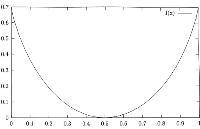
Figure 1-1: The rate function for coin tossing

we sometimes write equation (1.1) using the following notation,

F { M n ^ x )

Obviously, the rate function has to be non-negative everywhere, and it reaches zero at

the mean because the probability of this typical behaviour tends to 1. In the case of our

coin-tossing example, a graph of the rate function is shown in Figure 1.1.

C H APTER 1. INTRO DU CTIO N

4

half the time and with a frequency of 0.8 the rest of the time.

In a more general situation, we can consider arbitrary stochastic processes and ask

whether some large scale property of the process, such as its empirical average, satisfies

a large deviation principle (LDP). In such cases, the heuristic argument above can break

down. For example,

heavy-tailed

processes, where, for each individual random variable,

the probability of unusual behaviour does not decay quickly, may satisfy LDPs on hyper-

exponential scales. In such cases, the deviation can be caused by the action of a single

random variable, rather than being spread over the entire history of the process, and the

rate function will not necessarily be convex.

The precise definition of an abstract LDP is somewhat technical and is covered in Chap­

ter 2. In the general case, instead of a sequence of laws of empirical averages, as for

coin-tossing, we look at an arbitrary sequence of measures and examine the logarithmic

asymptotics of the sequence on certain sets, against some specified scale. Roughly speaking,

the LDP holds when

lim

log P(

e -B) = - inf 7 (x ),

n —>oo

l/^

xeB

for

B

in some suitably defined class of sets.

1.2

W hat we talk about w hen we talk about random sam ­

pling

We have in mind a situation where a stochastic process can only be observed at certain times,

which are governed by some other random process. Thus the observer has only partial infor­

mation about the behaviour of the underlying process. As a concrete, if somewhat artificial,

example, consider the transit time along some city bus route, subject to unpredictable vari­

ations, as the underlying stochastic process. Consider also an individual commuter who,

subject to random whims, may choose alternatives to the public transport provided. We

could describe this situation as a random sampling of the transit time process. The process

consisting of the commuter’s transit times on public transport is obviously related to the

underlying process, but there is also an effect due to his random decision process.

C H APTER 1. INTRO DU CTIO N

5

the

observation process, and the time of the n^^ observation is usually denoted T„.

Nt

typically refers to the number of observations before time

t. In th at case, the

observed

process, consisting of the sequence of samples, is defined by

Yn := X t^ .

We are interested in finding out how the random sampling transformation affects the large

deviations properties of the underlying process, and, if possible, relating the rate functions

of {Xt} and {T„} to that of {Vn}. We would expect th at the asymptotic properties of the

process would be changed by this operation, since the number of ways in which an event can

happen is greatly increased by the addition of random time intervals between observations.

For instance, to achieve some deviation of the observed process, either the underlying process

could behave in a similarly deviant fashion and the observations be typically distributed,

or the underlying process could behave in a more typical manner and the deviation be

attributable to an unusual sequence of observations. Hence, to use the cost analogy, we

can see there should be some trade-off of the cost of atypical behaviour of the underlying

process against that of atypical behaviour of the observation process.

We start by considering a concrete example where the underlying process is a Markov

process and the times between observations are independent. In this case, the resulting

process can be completely described by a Markov chain, the large deviation properties of

which are well-known. When the state space of the Markov process consists of only two

values, and the inter-observation times are exponentially distributed, we can identify the

Markov chain precisely. This we describe in Chapter 3, where we use this result to come up

with a new, if rather unwieldy, formula for the rate function of a 2-state Markov chain.

In so doing, we rely on a formula which is at the centre of Chapter 4 where we relax the

conditions on the underlying process while keeping the Poisson structure of the observation

process. In this case, we can derive a formula which describes the rate function for the

observed process in term s of the underlying one.

CHAPTER 1. INTRODUCTION

drawn from the first m (n) elements, where

6

lim

= ^ ,

for /? € (0,1).

n->oo m (nj

Its distribution is such that every distinct set of n samples in

,m} is equally likely.

When the empirical average of the underlying deterministic sequence converges, they show

th at the resulting stochastic process obeys an LDP and they provide a formula for the rate

function. They generalise this analysis to consider empirical measures.

For the most part, we restrict our intentions to continuous time processes. When the

arguments used in Chapter 4 are converted to the discrete time case, the observation pro­

cess we choose has geometrically distributed inter-observation times, this being the closest

analogue of the Poisson process. This process conforms to the conditions for the LDP de­

rived by Dembo and Zeitouni, and, in that case, the rate function they derive occurs as an

intermediate step in the derivation of the rate function in the discrete time random sampling

transformation.

C hapter 2

Large deviations

The aim of this chapter is to provide an abstract introduction to some of the technical aspects

of the theory of large deviations and to define some concepts th at we will use throughout the

remaining chapters. We use the framework described and developed by Lewis and Pfister

in [7]. A minor, but potentially confusing, difference is th at in our discussion of the LDP,

the rate function is defined to have a different sign to th at of the rate function in [7]. We

do this because, outside of this chapter, we are only interested in the large deviations of

probability measures, whose logarithm is always non-positive. For this reason, we follow the

convention of the probability literature and choose to deal with non-negative rate functions.

This implies th at the rate function be lower, rather than upper, semi-continuous.

In Section 2.1, we define some of the terminology we will use and state some simple results

regarding the properties of semi-continuous functions and their relation to set functions. In

the following section we describe the incremental approach to proving an LDP which is

explained in some detail by Lewis and Pfister in [7]. In Section 2.3, we investigate the

general form of Varadhan’s theorems, originally proved by Varadhan in [10]. We prove

these theorems, in a more restricted setting, within the framework of [7]. In Section 2.4, we

review some issues relating to stochastic processes and the LDPs deriving from them.

The material in Sections 2.1 and 2.2 is not original, begin merely a summary of [7], b u t

in Section 2.3, where proofs are provided either the result or the method of proof is believed

to be novel.

C H APTER 2. LARG E D EVIATIO NS

8

2.1

Sem i-continuity, set functions and level sets

In advance of discussing the definition of an LDP, it is helpful to gather together some facts

about semi-continuous functions, set functions and the links between them. Let X be a

Hausdorff topological space, and let

G denote a generic member of Q, the collection of open

sets.

For a function / : X ^ E, its

level sets are those of the form

{x : f { x )

<

a},

for some finite a. We say that / is lower semi-continuous (Isc) iff all its level sets are closed.

/ is upper semi-continuous (use) if —/ is Isc, or, in other words, if all sets of the form

{x : f {x)

^ a} are closed, for finite

a.

A set function is a function from a class of subsets of X

to E. We define two operations,

which transform set functions into real-valued functions on

X

and vice versa. We only

concern ourselves with set functions whose domain includes

Q.

D efinition 1

For a set function c, the inf-derivative

of c is

{x)

inf c[G] = {c[G]

: G £ Q , x E G} .

For a function / : X -> E,

the sup-integral

of f is

'^/[G] :=

sup f i x ) .

Using this terminology, for an arbitrary function we define semi-continuous regularisations.

D efin ition 2

For an arbitrary function f : X

R, we define the use regularisation by

fO

and the Isc regularisation by

f . : = i i r

C H APTER 2. L A RG E DEVIATIONS

9

L em m a 2.1

/

is use if and only if

=

f-Proof.

For any a, we define

Ga •— {x :

f {x) < a}.

Assume first that / is use. Since

f ^ ^ f

automatically, we need only prove the opposite

inequality. Fix x, and take any a > f {x). Since / is use,

Ga G Q, and of course

[Go] ^ o-

Therefore, because

Ga B x,

f ^{x)

= inf sup /(y ) ^

a.

Since this holds for all

a > f {x),

we can conclude th at

f ^

^ / .

On the other hand, assuming th at /^ = / , we want to show th a t

Ga is open.

Ga =

<x :

inf sup

f{y) < a

=

\ 3 G 3 X such th at

G is open and G C Gqj- .

Thus

Ga is equal to its interior and so is open. Hence / is use.

□

For an arbitrary function, / , it can be shown, by a similar argument to th a t used in

proving the second part of the previous lemma, that (x :

f ^{x)

< a} is open for all

finite a.

Hence,

f ^

is always use. Of course, parallel statements hold true for the Isc regularisation:

/o is Isc for any / , and / itself is Isc if and only if / = /<>.

Using this characterisation of upper semi-continuity, we can show th at the inf-derivative

of c, a set function, is a use function by showing that for any a:,

{' ^cY{x)

<

^c{x),

and this follows from the fact that

sup inf

c\G'] ^ c[G],

V G 9 a:

CH APTER 2. LA RG E D EVIATIO NS

10

2.2

The vague and narrow path to the LDP

In later chapters, we will only be concerned with LDPs on

but for the present we wish

to define a more general setting in which to prove the extension to Varadhan’s theorem.

We consider a sequence of measures

on a HausdorfF topological space

X ,

equipped with a Borel structure. We denote the collection of closed sets by

T ,

and the

compact sets by

1C.

We let

denote a scale, an increasing sequence of positive real

numbers, diverging to +oo. We are interested in examining the exponential asymptotic

properties of these measures on this scale. To this end, we make the following definitions

m n [ B ] : =

:^logM„[5];

m[B] :=

limsupm„[jB];

n —> 0 0

rn\B]

:= lim in fm „ f5 l.

Using these definitions, we can state the abstract LDP as follows.

D efinition 3

{M„}

satisfies an LDP, on the scale

with rate function I : X ^ R, if

the following conditions are satisfied

(L D P l)

I is lower semi-continuous;

(L D P 2)

I has compact level-sets;

(L D PS)

- i n f / ( a ; )

^

m[G] ,

y O e Q ;

(L D P 4)

fn[F]

^ - i n f / ( x ) ,

F ^ T .

There is a general approach to showing the existence of a rate function for a given

sequence {(M^, V'„)} which relies on finding a function to satisfy a weaker set of conditions,

and then using topological arguments to show that this function qualifies as a rate function.

We make these weaker conditions precise in the following definition.

D e fin itio n 4 {M„}

satisfies a

vague

LDP on the scale

{Ki}

with

function I, if I sat­

isfies L D P l, LDPS and

CH APTER 2. LARG E D EVIATIO NS

11

In order to establish some useful conditions under which a vague LDP is guaranteed, we

define two new functions.

fi{x)

;=

inf m[ G] ,

— G B x

JI (x) :=

inf m [G] ,

called, respectively, the upper and lower deviation functions. This pair of functions can be

used to show the existence of the function I,

satisfying the vague LDP.

The inf-derivative of a set function is necessarily upper semi-continuous, which means

th at

—/£

and

both satisfy LD Pl. We also note th at the definition of ^ implies

sup /i (x) < m [G] , V G e ^ ,

and it is proved in [7, Lemma 2.5], via the principle of the largest term, th at

m [K] ^ sup

V K € /C.

Hence, if /i and

are equal, then the conditions for the vague LDP are met by the negative

of th at function. In this case, we define the Ruelle-Lanford (RL) function,

/i(x)

:= [i{x) =Jl{x) .

Of course, this merely reduces the problem of proving the vague LDP to showing the

existence of the RL function. However, there is a fact to note about the definition of the

upper and lower deviation functions which helps us to do this. If 6 is a base of Borel

neighbourhoods, then for all G G ^ there exists

B E B such th at

B C G. Since both m and

m are increasing set functions, this means th at (using

B

to denote a generic element of B)

u (x)

= inf

m [G]

= inf m [B] ,

JI (x)

= inf m [G]

= inf m [B] .

^ G 3 x ^ B a x ^

Hence, if we can show that for some such base,

B,

CH APTER 2. LARG E D EVIATIO NS

12

then we can conclude that the RL function exists. At several points, we will use this

technique in the case where

X

is

, where the open balls are a base for the usual topology.

In certain cases, it is possible to promote a vague LDP to a full LDP. This involves two

steps, the first is changing the scope of the upper bound by showing that the rate function

satisfies LDP4, rather than ju st LDP4’; the second is proving th a t the level sets of the

rate function are compact. W ith the strengthening of the upper bound from compact sets

to closed sets, we get what Lewis and Pfister term a

narrow

LDP. Some authors, such as

Dembo and Zeitouni in [4], define an LDP to be what we term a narrow LDP; they then

use the term

good

to describe a rate function with compact level sets.

If all closed sets are compact, then LDP4’ implies LDP4, and since the level sets of a

lower semi-continuous function are closed, by definition, we can move immediately from a

vague to a full LDP. In most cases th at will concern us in this thesis,

X

itself is compact,

in which case all closed sets are also compact. Therefore, in such cases, if we choose to

prove the LDP via showing the existence of the RL function, then that is in fact all th a t

we need to prove since its existence guarantees a vague LDP which leads automatically to

the full LDP. Lewis and Pfister show that, even if the space is not compact, the

exponential

tightness

condition guarantees th at a sequence satisfying a vague LDP will obey a full LDP.

D efinition

5

A sequence of measures,

{Mn},

is exponentially tight on the scale

{V'n}

if

there exists a sequence, {K n}, of compact subsets of X such that

lim

ffi[X\Kn\ = —oc .

n->oo

In [7, Section 5], they show th at if a sequence of measures obeys a vague LDP and is

exponentially tight on the same scale, then the sequence obeys a narrow LDP with the

same rate function. In the case where

X

is regular, this rate function is unique, and so is

equal to the RL function whose level sets are compact, which completes the conditions for

the full LDP.

2.3

Varadhan’s theorem

We now investigate a method of using an LDP for one sequence of measures to prove an

C H A P T E R 2. L A R G E D E V IA T IO N S 13

A s s u m p tio n 2.1 {M„}n^i is a sequence o f locally finite measures on a H ausdorff space X , which obey an LD P on the scale {Vn} with rate function I = —jj,, where /i is the R L function fo r the sequence.

We are interested in considering th e large deviations of a sequence of exponentially tilted measures, where we define

Jb

W ith suitable conditions on the sequence of functions {gn}i we can show th a t ^n)} satisfies an LDP. In keeping w ith the notation of the previous section, we define th e following functions.

:= :^ log M ^ '^ [5]

m^\B] := lim inf [5 ], H^ix) inf [G] ,

n->-oo — G 3 x

m^[B] := lim su p m n " [S ], Ti^ix) := inf [G] .

n —)-oo G 3x

T he result known as V aradhan’s theorem concerns the exponential asym ptotics of th e tilte d m easure applied to the whole space, [X].

Varadhan’s approach

In V aradhan’s original paper, [10], he imposes certain convergence criteria on the sequence of functions which ensure th a t the tilted measures, applied to the whole space, have the app ropriate exponential asym ptotics. In order to obtain th e upper bound, he also imposes a tail condition on the tilte d measures which ensures th a t th e functions do not grow too quickly. This condition is trivially satisfied by a sequence of functions which are uniformly bounded.

CH APTER 2. LARG E DEVIATIONS

14

V I

Ve > 0, there exists a neighbourhood, N

9 xq, such th at for all sufficiently

large n and

all x E N,

9n{^) ^ 9

(^0)

^ 5

V 2

Ve > 0, there exists a neighbourhood, N 3 Xq, such th at for all sufficiently

large

and all a;

9n{x) >

gixo) - e;

and the tail condition,

V 3

lim lim sup

l o g [

„ “ ^[L,oo)] = -

.

L->oo n-foo

Vn

Using these conditions, Varadhan proves the result in three stages. First, he proves the

upper bound.

T heorem 2.2

If condition VI holds at every x for the function g{x), and VS is satisfied,

then

m^[X] < sup {g{x) - I{x)} .

x ex

Next, he defines the set

X

to be the set of points in X

where condition V2 holds and this

gives the following lower bound.

T heorem 2.3

^ sup {c;(a:) - I{x)} .

These are then combined to give the result known as Varadhan’s theorem.

T heorem 2.4

I f condition V3 holds and there exists a function g \ X ^ B. satisfying

condition VI at every x such that

sup {g{x) - I{x)} = sup{(/(a;)

- I{x)} ,

x e X o ajGX

then

CHAPTER 2. LARG E DEVIATIONS

15

T h e L ew is-P fister approach

In the more common statement of Varadhan’s theorem, the sequence of tilted measures is

obtained from the original sequence by means of a single function,

= M® , (2.1)

where

g :

X —)■ K is some locally bounded function. This is the situation considered by

Lewis

and

Pfister in [7]. In the case where

g

is continuous, they show the existence of, and

identify, the RL function

jjP = ll + g^ (2.2)

and conclude th at the sequence satisfies a vague LDP. As explained in the previous section,

when the space is compact, a vague LDP is equivalent to a full LDP, and so they get the

following theorem.

Theorem 2.5

If X is compact then, for a locally bounded, continuous function,

g

:

X

—

>• M,

rn^[X] = rn^[X]

= sup {g(a:) -

I{x)} .

xex

They also show th at for an arbitrary Hausdorff space, this vague LDP can be promoted to

a full LDP by using Varadhan’s condition, V3.

In the remainder of this section, we wish to expand the approach taken by Lewis and

Pfister to cover the situation where the measures are tilted by a sequence of functions. We

also explore equivalent conditions to VI and V2.

A central lemma in the investigation of tilted measures, defined as in equation (2.1),

in [7, section 2], states that

[i{x)+goix)

<

<

J l{ x) + g ^ {x ),

l£{x) + go{x) ^ yP{x)

<

-Ji{x)+g^{x).

If

g

is continuous, then

g<> = g^,

and

C H APTER 2. LARG E DEVIATIO NS

16

and the existence of

fx

gives the vague LDP for {(IV!^,F„)} with the rate function given

in equation (2.2).

We can prove a similar lemma in the more general setting, but we require more than ju st

continuity of the limit function to attain equality. However, before imposing any conditions

on {^n}) a-iid without needing to assume th a t ^ = /Z, we can prove the following;

Lem m a 2.6

Let Qn be locally bounded and measurable for all n. Then the upper and lower

deviation functions for

are related to those for (Mn,F„)

by

~pp{x) <

Ti{x)+ inf lim sup sup

„ ( y ) ,

li^{x) ^

+ sup lim inf inf

gniv) ■

Proof.

The proofs of the inequalities are almost identical, so we will just prove the first.

For any open set

G,

m^[G] ^ m„[G] + sup

In fact, for

G D G' 3 x,

[G'] ^

[G'] + sup

(y),

mP [G'] ^

fn[G'] + lim sup sup

(y).

Taking the infimum over

G' and the supremum over

G,

ju®(x) ^ /7(a;) + inf lim sup sup

n{y).

□

{^n}-C H A P T E R 2. L A R G E D E V IA T IO N S 17

{Cg){x) ;= in f lim sup sup 5„(y ). G Bx n->oo 2/ec?

Lem ma 2.6 th en implies

H + {Sg) ^ ^ n + {Cg) ,

and hence equality of (Sg) (x) and (£g) (x) implies existence of th e RL function at x for the tilted sequence. Not surprisingly, it tu rn s out th a t th e conditions V I and V2 are sufficient to dem onstrate the equality of Cg and Sg, and in fact, they are also necessary.

L em m a 2.7

{Cg) (x) ^ g{x) <=> VI holds at x fo r g{x).

{Sg) {x) ^ g{x) V2 holds at x fo r g{x).

P ro o f. We check the details for the first equivalence by simply following the definitions.

{Cg) {x) < g{x)

<;=^ inf lim sup sup gn{y) g { x ) , G3x n —>oo 2/€u

V e > 0 , 3 G g 3 a : s.t. lim sup sup gn{y) ^ g{x) + e , n —>oo y€Gc

V e > 0 , 3 G e 9 x S.t. Ve ' > 0 , 3 iVff s . t . sup sup 9n(y) ^ 9(a;) + e + e ', \/S > 0 , 3 G s 3 X , Ns s.t. sup sup gn{y) ^ g{^) + S ,

n > N s y € G s V I holds a t X for g { x )

The proof of th e second equivalence is identical. O

CH APTER 2. LA RG E DEVIATIONS

consider

gn(x) = i n x + 2

—n x

a: ^ or a; ^ 0

The hm it of gn{x) is zero for all a;, b u t there does not exist G 9 a: for which supg„ is not G

ultim ately 1.

If th e conditions V I and V2 b o th hold at a point x E X w ith value g{x), then we say

th a t condition V is satisfied, where th e condition is stated as follows.

(V ) Ve > 0, there exists

G 3 x

N

e

V n

N

So, if we assume th a t condition V holds true a t a point x, we know from Lemmas 2.6 and 2.7

th a t the RL function exists there and is given by

H^ix) = iJ,{x)+g{x),

and if condition V is m et at every x € X , we know th a t the tilted measures obey a vague

LDP. If X is compact then, as explained before, V aradhan’s theorem is im m ediate; since we

know th a t X is also open, we can use the equal bounds provided by th e u pper and lower

deviation functions.

sup IjL^{x) ^ ^ fnP[X] ^ sup /i®(x),

Using th e observation in Lem ma 2.9, this can be sum m arised in th e following theorem.

T h e o r e m 2 .8 I f X is compact, then for a sequence of locally bounded functions gn : X —> K,

which satisfy condition V at all x E X

lim log f = sup {g{x) — I ( x ) } ,

n-^oo Vn J x xeX

where g(x) — lim n->oo

W hen th e space is not com pact, it is more difficult to apply th e style of argum ent used

C H A P T E R 2. L A R G E D E V IA T IO N S 19

L o ca lly u n ifo r m c o n v e rg e n c e

We now wish to detail some implications, an d provide alternative formulations, of condition

V.

W hen V holds at a point x, we know th a t given e > 0, there exists an open neighbourhood

G 3 X such th a t \gn{y) — 5(a:^)| < e for all y & G. Since all such G certainly contain x, we

obtain th e following n atu ral result.

L em m a 2.9

In order to make condition V easier to check we prove a couple of theorem s about the

convergence of sequences of functions. F irst of all we isolate th e convergence aspect of

V aradhan’s condition.

D efinition 6

uniform iff given e > 0 and x £ X , there exists a neighbourhood of G 3 x, and an N such

that,

\9n{y) - g{y)\ < e, ^ y £ G , n > N .

T heorem 2.10

only if condition V holds at every x E X .

Proof.

Lemma 2.9, we know th a t g is the pointwise limit of the sequence {^n}- For any e > 0,

condition V tells us th a t there exists G 3 x and num ber N such th a t

\9n { y ) - g { x ) \ < e, y y e G , n > N ,

<

y y €G,

n—¥oo

Hence g is continuous.

Now we wish to show th a t th e convergence is locally uniform. Consider e > 0 . Since g

is continuous there exists a set Gi 3 x such th a t

C H A P T E R 2. L A R G E D E V IA T IO N S 20

and, by condition V, there exists a set G2 3 x, and a number N such that

\ 9 n { y ) - g i x ) \ < V y G G2, n > i V .

Hence, as required

\ 9n{y) - g{ y ) \ < e, Vy e Gi n G2,n > iV.

The proof of the “only if” part is almost identical. Again, taJie e > 0 . Since g is

continuous, and the convergence of to g is locally uniform, we know there exist open

neighbourhoods of x, Gi and G2 and a number N such that

\ 9ni v) - g{y)\ < ^ , \g{y) - g{x)\ < € , V y e G i n G2,n > iV,

\9n{ y ) - g{x)\ < 2e , V y e Gi n G2,n > iV,

which shows that condition V is satisfied. □

For characterising the convergence of sequences of functions, uniform convergence on

compact subsets is a more common criterion than locally uniform convergence. T he following

theorem shows that it is, in fact, sufficient, and in the case o f locally com pact spaces,

necessary.

T h e o r e m 2 .1 1 If the convergence to g, of the sequence of functions {gn}> is locally uniform,

then it is uniform on compact subsets of X .

In a locally compact space, if the sequence converges uniformly to g on compact subsets,

then the convergence is locally uniform.

P r o o f. Assum e first that the convergence is locally uniform. Then, given a compact subset

i f , and e > 0, then for every x E K , we can find a neighbourhood G^ 9 x, and a number

Nx, such that

l f f n { y ) - 5 ( y ) l < e , M y e G x , n > N x .

CHAPTER 2. LARG E DEVIATIONS

{Gxii- ■

■,

whose union contains

K.

Hence

21

\9n{y) -g{.y)\

< e,

Vy G

K , n >

max{JVxi, . . . , ■

On the other hand, if X is locally compact then every point, x, has a compact neigh­

bourhood, say

Kx-

Since convergence is compact on this subset and it contains an open

neighbourhood, we can conclude th at condition V holds at this point.

□

2.4

Stochastic processes

The LDPs which will concern us in the following chapters derive from either the empirical

averages, or empirical measures, of stochastic processes.

Em pirical Averages

For a stochastic process, {1^}, taking values in S, we might be interested in the large

deviation properties of the sequence of measures, {M„}, defined by

M„ [B]

^ ^

^ ^

Borel sets

B.

These measures are the laws of the empirical means. We will usually only consider the

empirical average of a 2-state process. In that case, the average at time n tells us the

number of those

n

random variables in each of the states; for instance, if S = {0,1}, then

the partial sum, Yi

is the number of times the process has been in state 1.

Em pirical M easures

For a process where the cardinality of the state space is greater than two, the partial sum is

likely to hide the percentage of the total time spent in each state. To capture the same type

of information about such a process, we construct the empirical measure. The empirical

measure of a discrete-time process, {V^}) is a measure on E, defined by

C H APTER 2. LA RG E D EVIATIO NS

22

In order to examine the large deviations of the laws of these measures, we need to specify a

topology on the space of measures,

M.

(S). In general, this space can have many topologies,

but we will only concern ourselves with processes taking values in a finite set. We let the

cardinality of S be M and, to simplify notation, we take E to be the set {1, . . . , M}. In this

case, each measure can represented as a sum of Dirac measures;

M ^ M [{i}] Si ■ ^ i^M

In this way, to each measure, we can associate a vector in

We define the set of all

probability vectors

r = {y € ]R+ : yi + •. • yjw = 1} ,

and the natural mapping to this set from the space of measures,

C

: M ( S ) ^ r ,

C :

/i 1-^ ^/i[{l}],...

.

We will refer to the components of the image vector as the

of the measure. We

take r to be equipped with a topology which is the relativisation of the usual topology on

. Since

C

is bijective, we will talk about a measure and its coordinates interchangeably.

In particular, we will refer to an LDP on F, for the coordinates of the empirical measure,

as an LDP on

A i

(S) for the empirical measures.

R elative entropy and accessib ility

For the purposes of defining some further notation, we consider a E-valued stochastic process

consisting of independent random variables sharing a common distribution on S;

C H A P T E R 2. L A R G E D E V IA T IO N S 23

Let yUn be th e empirical measure of th e process at time n, and define := C(fin) so th a t

O f course, th e components of this vector m ust be of the form ^ for fc G { 0 ,1 ,... n}, and so

we define the following finite subset of F, which contains th e attainable vectors at tim e n,

Tn = {q S r : nqi G N for all 1 ^ i ^ M } .

Thus, we have th a t for y G r \ r „ , P ^ ~ ^ ~ ^ for

q

This function occurs frequently in C hapter 4, and so, w ith exponential asym ptotics in m ind,

we define, for

q

ft„(q,v)

:= i

P ( U(”) = q ) = i log

-

(q| v)

- ff

(q)

, (2.3)

where H

(u|

u

u

M

H { u \ v )

Vi

i=l ®

and -ff(u), th e entropy of u G F is given by

M

H { u ) : = - ' ^ U i l o g U i .

The relative entropy, i / (• | v ) , is the rate function for th e laws of the empirical measures

of {Yn}. We also extend /i„ to a set function by the following definition. For B , a Borel

subset of F, we define

fc „ (S ,v ) ;= i l o g l 5 3 I ,

^ \qeBnr„ /

C H APTER 2. LA RG E D EVIATIO NS

24

P

Lastly, we wish to define the set of probability vectors from which a given vector is

accessible.

This definition helps to simplify some technical details of the proofs in Chapter 4.

For a process such as {Fn}, it is possible to choose v, the vector describing the distribution,

zero. We say that a state is accessible from v if it has a non-zero probability of being visited.

A support for a probability measure is any set whose measure is 1. Similarly, we define the

support, 5 (v ), of a probability vector, v, to be

We have, therefore, th at for v G .A(x), Uj = 0 => Xj = 0.

Continuous tim e processes and m easurability

Although the process resulting from the random sampling transformation is necessarily a

discrete time process, we will also deal with continuous time processes. The underlying

process in many cases will be indexed by R-|_, rather than N. The statem ent of the LDP in

continuous time is almost identical to that in discrete time. For example, we can define the

empirical average of a process

by

and then look at an LDP for the sequence

{Ci^Zt))

the scale

t.

The discussion of LDPs earlier in this chapter goes through analogously when the se­

quence of measures is indexed by R rather than N. However, there is a potential difficulty is

in the definition of quantities such as the integral in equation (2.4). In order to guarantee

th at functions such as

Zt

are measurable, we need to impose an additional measurability

constraint on the process {Xi}. In [5], Doob defines measurability of a stochastic process

to be on the boundary of F. In th a t case, the probability of visiting certain states will be

and using this, the set of vectors from which x is accessible is given by

^ (x ) := {v e F : 5(x) C 5(v)} .

CH APTER 2. LA RG E DEVIATIO NS

25

in the following way:

D efinition 7

A stochastic process

{XtjtgR,

defined on the probability triple

is

measurable iff the function X

: O x K ->• K,

where X{u},t) = Xt{u}), is measurable with

respect to the product space

x R,

x B, X x

Leb).

Doob discusses stochastic convergence properties th at guarantee measurability, and shows

how measurability of a stochastic process ensures th at integrals of the process, such as in

equation (2.4), are measurable.

Throughout the remaining chapters, we will assume th a t all continuous time processes

are measurable.

The Poisson process

In this section, we wish to gather a few facts about the Poisson process, which we will have

need of in Chapter 4.

Consider a Poisson process with rate

a, {Nt}teM.+i

defined on the probability triple

We will be principally interested in the related process,

which defines

the sequence of jum p times.

Since

Nt

is Poisson, {T„+i — T„} are independent and are all exponentially distributed with

parameter

a.

Using this simple structure, it is not difficult to see th at the joint law of

{ Ti ,. . . , T„} has a density given by

Of course, by integrating over the first n — 1 variables, we see th a t the law of T„ has the

density

We also make use of the fact th a t the laws of T „/n obey an empirical average LDP on

Tn =

sup{i

: Nt < n } .

(2.5)

the scale n. This can be easily seen from Cramer’s theorem (see, for example, [4, C hapter

C H APTER 2. L A RG E DEVIATIONS

26

given by

A(0) = logE e^^i,

= , ‘° « ( * )

+ 0 0 ,

V

Hence, we can conclude th at

{C^Tn/n)}

satisfy an LDP

Fenchel transform of A,

I r it)

= sup{i0 — A(0)} ,

e

— a t —

log(o;i) — 1.

(2.8)

The scaled cum ulant generating function

We made use in the previous section of the scaled cumulant generating function (sCGF);

this is a very useful tool in the theory of large deviations. In general, for a discrete time

process {X„}, the sCGF is defined by

A(0) := lim — logE exp

+ . . . +

,

7i->oo

n

\

/

where this limit exists. The usefulness of the sCGF stems from the fact th a t existence of

the rate function implies, by Varadhan’s theorem, existence of the sCGF, and furthermore

th at A is the Legendre-Fenchel transform of

I.

If, in addition,

I

is known to be convex,

then there is a duality and

I

is the Legendre transform of A. This is often the easiest way

to calculate the rate function.

6 < a

(2.7)

9

a .

Legendre-Chapter 3

Markov underlying processes

For this initial investigation of random sampling, we will restrict our attention to a specific

class of processes. If we examine random sampling in discrete time, we have the option of

choosing an uncorrelated underlying process, for instance a Bernoulli process. However, for

any choice of observation process (with strictly increasing observation times), it is not hard

to see th at the observed process is identical in distribution to the underlying process. So,

in order to have a non-trivial transformation to examine, we work with a correlated process

and choose a Markov process as a relatively simple example.

In fact, we choose to work in continuous time since, despite some additional technical

considerations, the calculations are more tractable. We will use a Poisson process to deter­

mine the sequence of observations and restrict the underlying process to lie in the class of

finite state Markov processes. An almost identical analysis can be carried out in discrete

time if we replace the continuous time Markov process by a Markov chain and the observa­

tion process by a counting process whose inter-arrival times are geometrically distributed.

3.1

R andom ly sam pled Markov processes

Let

P) be a probability triple. W ith respect to this triple, we denote the time of the

observation by the random variable

and the number of observations before time

t

by

Nt,

where

Nt

:= sup

{ n : T n

.

C H APTER 3. M A R K O V UNDERLYING PROCESSES

We also define the inter-observation process,

by

28

W fi • — '^ n ^ n - 1 )

where To := 0.

A ssu m p tion 3.1

The inter-observation times {Wn} are independent and share a common

distribution with W , an almost surely bounded random variable taking values in

K_)_.

We denote the underlying process by

and its countable state space by S. For

convenience we take S to be a copy of N. We define

:=

and

:= a {Xs : s ^

A ssu m p tion 3.2

{ Xf } is a time-homogeneous Markov process with transition function

F{ i , j ; t ) : =

P(

Xg+t = j

|

=

i)

,

Vs

^

0.

The sample process is then given by

: = X t^ .

We are interested in finding out how the correlation structure of {Xj} is related to that

of {yn}- As shown in the following theorem, the Markov character is preserved by the

sampling.

T heorem 3.1

{yn}neN

is a Markov chain with transition matrix

f,j-.= E F { i , r , W ) .

Proof.

We wish to show th at for any

G S,

CHAPTER 3. M A R K O V UNDERLYING PROCESSES

29

a { Y o , Y n )

is generated by the family V

consisting of all sets of the form

{w : F o M =

= in}

V is a partition of fi, and is countable due to the countability of S. Therefore, we can write

P { Y n + i = i n + i \ Y o , . . . , Y n ) { u ; ) =

Y 1

(3.1)

P { B )

{BeV:P{B)>0} ^

and

P ( l i + i = i» + i I M (3-2)

{ k € f ^ : P { Y n = k ) >0} '

We can calculate these functions explicitly. For an arbitrary set

B

in}

V

we can use Theorem 4.1 to write

P ( = *n+l} n -S )

~ P ( Yq — id, ■ ■ ■ 1 ^n+l ~ '^n+l )

=

J

Now, since

is a Markov process, we can rewrite the integrand as

P ( X o = *0) = ■*!, ■ ■ • = *n+l )

= P ( Xq = *0) • • • t Xfn ~ *n ) -P' (*n> *n+l) ^n+1 ~~ ^n) ■

This expression only depends on tn+i through the difference

{tn+i — tn) and so, since {T„}

C H A P T E R 3 . M A R K O V U N D E R L Y I N G P R O C E S S E S

30

P(

{^+1

— *71+1} n 5 )

= J ^ {T i,...,T n ) [ d t i X ■ ■ ■ ^ d t j i ) P { X Q =

= i i , . .. ,Xt„ = in)

poo

X / C ( ^ w ) { d w ) P i ' i ' n , i n + l ’, w )

J w=0

= P ( Y o = i o , . . . , Y n = i n ) ' ^ ( F { i n , i n + i ; W ) ^

= P { B ) E ( ^ F { i n , i n + i ; W ) ) .

By summing over

ij

6 S, for each j ^ n — 1, and taking

in = k,

we can also conclude th at

P { Y n + i = i n + l , Y „ = k ) = P { Y n = k ) E ■

Hence, using the equations (3.1,3.2), we can see that

P(

je s

□

In order to further our investigation, we now choose to be more specific about the

underlying process.

A ssu m p tion 3.3 {X*}

is a stationary 2-state process, taking values in

{0,1},

with transi­

tion function

F(i,r,t) =

n ^ O

where, with

Aq,Ai > 0,

Prom the condition th at {Xt} be stationary, we know th at its starting distribution must

CH APTER 3. M A R K O V UNDERLYING PROCESSES

Starting from this distribution, the process then consists of a sequence of alternate sojourn

times in states

and

respectively.

In the light of this further assumption, {^71}) being a stationary 2-state Markov chain,

is characterised by the two transition probabilities

a

:= P ( y

„+1

= 1| yn = 0 ) ,

d

= l )

By applying Theorem 3.1, we can calculate these probabilities in the case where the obser­

vation process is Poisson.

T heorem 3.2

I f W is exponentially distributed with parameter a then

^0

j

j

a =

---;---

and

a ■

Aq + A i -|- CK Aq + A i -|- Q;

Proof.

We first calculate

a.

Using Theorem 3.1, we can write

roo

a = E[e^^]^-^=

(3.3)

Jo

We first need to evaluate

e^^.

Because of the simple form of A, it is easy to see that

= ( - A o - A i ) A

= > A ^ =

( - A o - Ai r - ' A ,

and so.

^ { t A r

n!

n —O

1 0 \ g-(Ao+Ai)t — 1 / —Aq Aq

0 1 y

Ao + Ai

y

Substituting this in equation (3.3) gives

a =

(

1 -

ae-^^dt