The Continuous Analogy of Newton’s Method for Solving a
System of Linear Algebraic Equations
Tugal Zhanlav1, Ochbadrakh Chuluunbaatar1,2*, Gantumur Ankhbayar1 1School of Mathematics and Computer Science, National University of Mongolia, Ulan-Bator, Mongolia
2Joint Institute for Nuclear Research, Dubna, Moscow Region, Russia Email: *[email protected]
Received October 31, 2012; revised January 2, 2013; accepted January 9, 2013
ABSTRACT
We propose a continuous analogy of Newton’s method with inner iteration for solving a system of linear algebraic equations. Implementation of inner iterations is carried out in two ways. The former is to fix the number of inner itera- tions in advance. The latter is to use the inexact Newton method for solution of the linear system of equations that arises at each stage of outer iterations. We give some new choices of iteration parameter and of forcing term, that ensure the convergence of iterations. The performance and efficiency of the proposed iteration is illustrated by numerical examples that represent a wide range of typical systems.
Keywords: Continuous Analogy of Newton’s Method; Solving the System of Linear Algebraic Equations;
Convergence; Choice of Iteration Parameter
1. Introduction
We consider a system of linear algebraic equations .
Ax f (1) For a numerical solving of Equation (1) we consider an iterative process:
1
0 1
n n
n n n n
Bv r x x v n (2) Of course, the quality of iterative process Equation (2) essentially depends on the choices of matrix B and of iteration parameter n 0
Let H be a linear space of m-dimensional vectors. We will denote the Euclidean vector norm in H by , as well as the corresponding norm of matrices.
Theorem 1.1. Let Then a necessary
and sufficient condition
for the
0 n n
Av r n
r to be decreasing
rn1 rn
isthat
2
2
2 ,
0, , when , 0,
2 ,
,0 , when , 0. n n
n n n
n n
n n
n n n
Av r
Av r Av
I
Av r
Av r Av
n Proof. From Equation (2) we obtain
1
n n n
r r Av
Hence we have
2 2 2
1 [ 2(
n n n n n n n
r r Av Av r)]
(3)
The assertion follows from (3).
The interval In we call τ-region of convergence of
the iteration method (2). Thus we have to choose n
from this region. Moreover, it is desirable that the n to
be optimal in some sense. Further we will use well- known assertions to study the convergence of (2).
Theorem 1.2. [1]. LetSbeanm × mmatrix. Thenthe
successiveapproximations
n 1 n , 0,1, 2,
x Sx z n (4)
converge for each z R m and each x 0 Rm if and
onlyif
S 1 (5)
where
S isaspectralradiusofthematrixS. It is easy to show that the iteration process (2) can be rewritten as (4) with iteration matrix1 and
n
S E B A z B f1
n
(6)
Here E is an m × m unit matrix.
Theorem 1.3. [2]. Theiteration process (2) with
pa-rameter n givenby
2
n n n
n
Av r Av
(7)
posterioriestimateholdstrue:
1 2 0 0 ,
n n n
r q q q r (8)
where
22 2 ,
1 i i 1, 0,1,
i
i i
Av r
q i
Av r
,n1.
We call the nonzero value of n defined by (10) the optimal one in the sense that it yields the minimum value of functional rn1 .
2. The Continuous Analogy of Newton’s
Method
The continuous analogy of Newton’s method is also ap-plicable to (1) and leads to [2]
n n
Av r (9a) n1 n , 0,1,
n n
x x v n (9b) It should be mentioned that not only the convergence, but also the convergence rate of iteration (9) depends on the choice of the parameter n. We have the following:
Lemma 2.1. The sufficient condition for rn to be
decreasingis 0n2,n0,1, 1
Lemma 2.2. Suppose that n2 for all .
Then the iterationprocess (2) givestwo-sided approxi-mationsto
0
n
x, i.e.,
1 2m1 2m 0 if 0
x x xx x xx
or
0 2m 2m1 1 if 0 .
x x xx x x x
.
x
The proofs are immediately followed from the equalities
1
1 1 , 1
n n
n n n n
r r x x x
At each step of iterations one can solve the system (9a) by means of some iterative methods. We call this inner iteration. We consider the following decomposition of
A:
1 2,
A A A
in which the matrix A1 is simple and invertible. For finding the correction vn we use inner iteration
1 1
1 2 , 0, 0,1,
e e
n n n n
A v r A v v e (10)
Theorem 2.3.Supposethat
1 2 1 1,
C CA A (11)
Thenthe inneriteration (10) convergesandholdsthe followingestimate
1 1
1 1 , 0,1,
k k
n n n
C
v v A r k C
(12)
Proof. The linear system (10) can be rewritten as
E C A v
1 n rn. (13) By assumption (11) there exists
E C
1 and the following series representation is valid
1
0
1 j j.
j
E C C
(14)Then from (13) it follows that
1 1
0
1 j j
n n
j
v A C r
r
(15)
In a similar way, from (10) we have
1
1 0
1
k j
k j
n n
j
v A C
(16)From (15) and (16) immediately follows (14).
The estimate (12) means that the inner iteration (10) converges under condition (11). In real computations we have to terminate the inner iteration before convergence. We will restrict the number of inner iteration by k. Then the whole iteration process looks like:
1 1
1 2 , 0, 0,1, , ,
l l
n n n n
A v r A v v l k (17a)
n1 n k , 0,1 n n
x x v n (17b)
We now formulate the convergence theorems for these methods.
Theorem 2.4.Supposethatthecondition (11) is
satis-fiedandtheiterationparameter n isgivenby
2 ,
k
n n
n
k n
Av r Av
(18)
Then the iteration process (17) converges for any
0,1,
k andforarbitrarychosenstarting x 0 .
Proof. We rewrite the iteration process (17) as (2)
with
1 10
1 k
j j
j
B C
A
By Theorem 1.3, such a process converges if we
choose n by (7), in which the n is replaced by .
Obviously the number k may be different for each n. From (12) it is evident, that it suffices to restrict the number of inner iteration only by k = 0 or 1, when the residual norm
v vn k
n
r is small enough.
Theorem 2.5.Supposethatthecondition (11) issatis-
converges forany and for arbitrary chosen starting
0,1,
k
0
x . Thefollowinginequalityholds:
1
n n
r rn , 0n 1
rn 1(19)
Proof. From (17) we get
1 .
k
n n n n
r r Av
Using (11) and (16) we rewrite the last expression as
1 1k 1 k 1n n n
r1 E C
0 n
(20)
If , then from (20) we obtain
1
1 , 1 1
k
n n n n n
r r C
1
According to (11), we have 0n . The
conver-gence of (17) follows from (19).
Corollary 2.6.Letthecondition (11) fulfill, and n is
givenby [3]
1
1 0
min n ;1 , 1, 2, , 0.1.
n n
n
r
n r
Thentheiteration (17) converges.
Remark 2.7.InproofsofTheorems 2.3-2.5 thecondi-
tion (11) isessentiallyused. Inparticular, itmaybeful- filled if the matrix A ofthe system (1) isa strongly di- agonallydominantandA1ischosenas
1 diag 11, , mm .
A a a
Theorem 2.8.Supposethatthecondition (11) is
satis-fied and that the eigenvalues of matrix are real. Thenthespectralradiusofiterationmatricesofthe iterations (17) is decreasing with respect to k when
1 1 2
DA A
1
n
.
Proof. The iterations (17) can be rewritten as (4) with
iteration matrices
1 11 1k k
k n n
S E D (21)
We denote by
D the eigenvalues of D. If n1, then
1 11k k k
S D
Therefore, we have
k 1k
S D
By virtue of (11) we obtain
C C 1. Since the spectrums of matrices C and D coincide, we also have
D 1
By definition we get
1
1
max max
max max
max ,
k
k k
k
k k
S S D
D D
D S
which is valid for all k1, 2, Thus we have
Sk
Sk 1
S1
S0 1. (22)
Obviously, from (21) it is clear that k is a continu-ous function of n
S
. Therefore, (22) is valid for n1
. The iteration (17) with a few small k represents a spe-cial interest from a computational view point. Moreover, it is worth to stay at (17) with k = 0 in detail. The itera-tion (17) with k = 0 and 1 11 mm leads to the well-known Jacobi iteration with relaxation
parame-ter n
,diag ,
A a a
. It is also known that [1] the Jacobi method with optimal relaxation parameter
min max 2 2
opt
(23)
converges under the assumption that the Jacobi matrix has real eigenvalues and spectral radius less than one. Here by min
1 1 2
B A A
and max denoted are the smallest and largest eigenvalues of B. Fortunately, we can prove the convergence of Jacobi method with rela- tion parameter under a mild condition than the above mentioned assumption. Namely, we have.
Corollary 2.9.Supposethatthe condition (11) is
sat-isfied. Then the Jacobi methodwith relaxation parame-ter:
0
2 0
, ,
n n n n
n
n n
Av r E C r r
Av E C r
(24)
converges for any starting.
From (24) it is clear that the relaxation parameter changes depending on n. Therefore the iteration (17) with
k = 0, and A1diag
a11, , amm
and with n givenby (24) we call nonstationary Jacobi method with opti-mal relaxation parameters. The iteration (17) with k = 0 and with a lower triangular matrix A1 leads to Gauss- Seidel with one parameter.
The Formula (18) can be rewritten as:
1
2 1
, ,
n n n
n
AB r r AB r
(25)
where AB1 E
1k1Ck1 From this it is clear that1
n
as k . This means that whole iteration (17) with the parameter given by (18) converges quadratically in the limit.
Since n1, as , then τ-region of conver-gence for iterations (17) leads to
2
2 ,
0; 0; 2
k
n n
k n
k n
Av r I
Av
. The number of outer iteration n depends on the num-ber of inner iteration k, i.e., . In general, n is a decreasing function of k, i.e., k
n n
nk1 nk
On the other hand, the iteration (17) can be considered as a defect correction iteration [1]
1 1
1 1
approx , approx ,
n n
n n
x x A r B A (26)
where 1 defined by approx
A
1 1 2
approx 1 1
k k
A A E C C C (27) 1
approx
A is a reasonable approximation to A1 since 1
1 1 1 1
approx 0
1
k
A C
A A
C
(28)
for large k. The choice of parameter n given by (25)
allows us to decrease the residual norm from iteration to iteration. By this reason we call (26) as a minimal defect (or residual) correction iteration.
From (26) it follows that
11 approx
n n
r E AA r
n (29)From (29) and
11 2 1, 2 1
A A A E C A C A A , it
follows that
11
approx 1 1
k k
n n n
E AA E C 1
. Therefore we have
1
1
1approx 1 1
k k
n n n
E AA C
This means that the spectral radius of matrix
depends on the number of inner iteration
k, i.e., . Therefore we have as , because
1 approx
n
E AA
k
k n1 as k and from (11)
k 0
C C 1
Above we considered the cases, where the inner itera- tion number k is fixed at each outer iteration. It is desir- able that the termination criterion for the inner iteration must be chosen carefully to preserve the superlinear convergence rate of the outer iteration. We stay at this problem in more detail. When 1, the iteration (17) is, indeed, inexact Newton (IN) method for (1). Therefore, iteration (17) with parameter n given by formula (18)
we call inexact damped Newton method (IDN). Accord- ing to IN method [4,5], we must choose n
0,1
and continue the inner iteration until satisfy the condition
1 , , 1, 2,
e e e
n n n n n n
r r r Av r n (30)
Thus (30) is a stopping criterion for inner iteration (17a). There are several choices of forcing term n in
inexact Newton method [4-6]. For examples, in [6] two choices of n were proposed:
1 1
1
1
1 , when
1
, when 1,
n n n n
n n n
n n
n
1,
(31)
with
1 ,
n n
n
r r
and
1 , 0,1,
n n n
(32)
Since we have formula (18) for n, one can use the
second choice (14) with no additional calculations. We can also use formula for 2
1 1
n
n
r
[7]. There-
fore, according to (32), we get
1 1
1 1
n n
n
r r
(33)
3. Numerical Results
The quality of the proposed iteration was checked up for numerous examples. We express the matrix A as
,
L U
A D A A
where Ddiag
a11, , amm
, and AL, AU are lower and upper triangular matrices, respectively. All examples are calculated with an accuracy 107n
Ax f .
The numerical calculations are performed on Acer, CPU 1.8 GHz, 1 GB RAM, and using a software MAT-LAB R2007a for the Windows XP system.
Example 1. We consider a system of Equation (1)
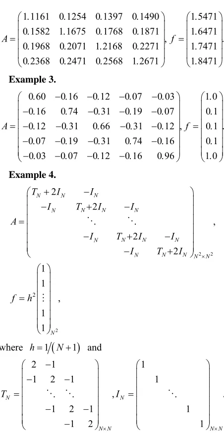
with matrix A and f given by
2 1 0 5
1 4 1 1 0
, 6 ,
1 4 1 1 0
1 2 m m 0 5 m
A f
which was solved by the proposed iteration method (17), (18). For comparison, it was solved by Jacobi and suc-cessive over relaxation (SOR) iterations with a parameter
opt
.
1 1161 0 1254 0 1397 0 1490 1 5471 0 1582 1 1675 0 1768 0 1871 1 6471 0 1968 0 2071 1 2168 0 2271 1 7471 0 2368 0 2471 0 2568 1 2671 1 8471
A
f
f
Example 3.0 60 0 16 0 12 0 07 0 03 1 0 0 16 0 74 0 31 0 19 0 07 0 1 0 12 0 31 0 66 0 31 0 12 0 1 0 07 0 19 0 31 0 74 0 16 0 1 0 03 0 07 0 12 0 16 0 96 1 0
A
Example 4.
2 2
2 2
2
2
2
2 1
1
1 1
N
N N
N N N
N
N N N
N
N N
N N N
N
T I I
I T I I
A
I T I I
I T I
f h
where h1
N1 and2 1 1
1 2 1 1
, .
1 2 1 1
1 2 1
N N
N N N
T I
N
Such a system arises in discretization of two dimen- sional Poisson equation [8]:
, 1, ,
0 , 1 ,
0 on .u x y D x y x y u D
The exact value of u
1 2 1 2
is [9]
4 2 2
, 0 1 1 , 2 2
1 16
π 1 2 1 2 1 2 1 2
0.0736713
u
(34)
The properties of matrix for examples 1-4 are shown
in Table 1. From this we see that the considered exam-
ples represent a wide range of typical systems.
The numbers of Jacobi and SOR iterations versus the dimension m of example 1 are presented in Table 2.
Here k is the number of inner iteration in (17) (18). From this example we see that the proposed iteration (17), (18) can compete with SOR iteration with optimal relaxation parameter and seem to be superior to the Jacobi iteration. The behavior of the iteration parameter n given by (18)
at m = 10 is explained in Table 3. From this we see that
the iteration parameter n tends to 1 as k increases.
The number n of outer iteration (17), (18) with fixed number k of inner iterations, and CPU time for examples 2 and 3 are shown in Table 4. From this we see that they
are in example 2 considerable less than example 3. This
explained by reason that matrix of this system has a strictly diagonally dominant. The number n of outer it- eration, the total number k of inner iteration when forcing terms n was chosen by formulas (32) and (33), and
CPU time are displayed in Table 5. Here it is observed
similar situations as in the previous case.
Monotonic convergence of the calculated values
1 2,1 2
hu to exact value (34) versus the dimension N
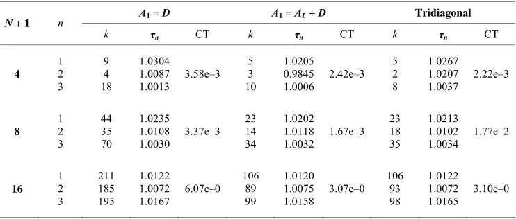
of the example 4 is shown in Table 6. The number n of
outer iteration with fixed and unfixed number k of inner iteration and CPU time versus the dimension N of the
example 4 are presented in Tables 7 and 8, respec-
[image:5.595.58.284.76.513.2]tively.
Table 1. The properties of matrix for examples 1-4.
Matrix Example
Symmetric Diagonally dominant Sparse
1 + + +
2 – + –
3 + – –
[image:5.595.307.539.399.480.2]4 + – +
Table 2. The numbers of Jacobi and SOR iterations versus the dimension of example 1. Here is the number of inner iteration in (17), (18).
m k
Iter. A1 = D Jacobi method A1=AL+D SOR
m/k 0 1 2 3 0 1 2 3 ωopt
10 16 10 9 6 30 12 7 5 4 12
100 18 9 8 5 32 14 7 5 4 17
1000 17 9 8 5 34 14 7 5 4 18
Table 3. The behavior of the iteration parameter τn given by (18) for example 1. Here n and k are the numbers of outer and inner iterations in (17), respectively.
n/k 1 2 3
1 1.031939 0.994921 1.000760
2 0.998348 1.001490 0.998875
3 0.988243 0.999830 1.000464
4 0.989728 1.011261 0.999378
5 1.014757 1.004592
6 1.024398
[image:5.595.307.539.529.589.2] [image:5.595.308.539.638.735.2]Table 4. The number n of outer iteration with fixed number k of inner iteration, and CPU time CT for examples 2 and 3.
Example 2 Example 3
A1
k=0 k=1 k=2 k=0 k=1 k=2
D CT n 1.5e–3 39 9.2e–4 17 8.6e–4 13 8.6e–4 196 6.9e–389 3.1e–356 AL + D CT n 6.7e–3 14 4.9e–4 5 4.5e–4 13 3.3e–4 92 2.7e–358 2.3e–341
SOR CT n 1.3e–3 8 5.1e–3 35
Table 5. The number n of outer iteration, the total number k of inner iteration when forcing terms ηn was chosen by formulas (32) and (33), and CPU time CT.
A1 Example 2 Example 3
CT 1.61e–3 1.07e–2 (33)
n (k) 4 (12) 5 (188)
CT 1.72e–3 1.08e–2
D
(32) n (k) 5 (11) 5 (135)
CT 1.10e–3 7.53e–3 (33)
n (k) 4 (5) 5 (94)
CT 1.11e–3 7.42e–3
AL + D
(32)
n (k) 4 (4) 4 (92)
4. Conclusions
Our method with inner iteration is quadratically conver- gent and therefore it can compete with other iterations such as SOR with an optimal relaxation parameter for a strictly diagonally dominant system. Moreover, our method is also applicable not only for the system with a strictly diagonal dominant matrix, but also for system, the matrix of which is not Hermitian and positive definite.
[image:6.595.58.292.265.362.2]This work was partially sponsored by foundation for science and technology of Ministry of Education, Culture, and Science (Mongolia).
Table 6. A comparison of the calculated values u(1/2, 1/2) and an exact value (34) versus the dimension N of the ex-ample 4.
N + 1 u(1/2, 1/2)
4 0.070312
8 0.072783
16 0.073446
32 0.073615
[image:6.595.111.487.401.539.2]Exact 0.073671
Table 7. The number n of outer iteration with fixed number k of inner iteration, and CPU time CT versus the dimension N of the example 4.
A1 = D A1 = AL + D Tridiagonal
N + 1
k = 0 k = 1 k = 2 k = 0 k = 1 k = 2 k = 0 k = 1 k = 2 SOR
4 CT n 2.5e–3 64 1.3e–3 20 1.4e–321 1.3e–332 8.8e–415 8.1e–411 1.2e–339 8.3e–416 7.6e–4 12 1.3e–3 11
8 CT n 1.4e–2 267 9.6e–3 60 1.2e–387 6.7e–3124 3.9e–360 4.2e–340 7.9e–3149 2.8e–340 3.6e–3 47 6.1e–3 23
[image:6.595.114.485.577.735.2]16 CT n 5.9e–1 1010 1.4e–1 159 3.0e–1328 2.8e–1476 1.7e–1214 1.3e–1137 2.9e–1546 1.0e–199 1.8e–1 183 1.0e–1 46
Table 8. The number n of outer iteration with unfixed number k of inner iteration, the itration parameter τn, and CPU time CT versus the dimension N of the example 4.
A1 = D A1 = AL + D Tridiagonal
N + 1 n
k τn CT k τn CT k τn CT
4
1 2 3
9 4 18
1.0304 1.0087
1.0013 3.58e–3 5 3 10
1.0205 0.9845
1.0006 2.42e–3 5 2 8
1.0267 1.0207
1.0037 2.22e–3
8
1 2 3
44 35 70
1.0235 1.0108
1.0030 3.37e–3 23 14 34
1.0202 1.0118
1.0032 1.67e–3 23 18 35
1.0213 1.0102
1.0034 1.77e–2
16
1 2 3
211 185 195
1.0122 1.0072 1.0167
6.07e–0 106
89 99
1.0120 1.0075 1.0158
3.07e–0 106
93 98
1.0122 1.0072 1.0165
O. Chuluunbaatar acknowledges a financial support from the RFBR Grant No. 11-01-00523, and the theme 09-6-1060-2005/2013 “Mathematical support of experi-mental and theoretical studies conducted by JINR”.
REFERENCES
[1] R. Kress, “Numerical Analysis,” Springer-Verlag, Berlin, 1998. doi:10.1007/978-1-4612-0599-9
[2] T. Zhanlav, “On the Iteration Method with Minimal De-fect for Solving a System of Linear Algebraic Equations,” Scientific Transaction, No. 8, 2001, pp. 59-64.
[3] T. Zhanlav and I. V. Puzynin, “The Convergence of Itera-tions Based on a Continuous Analogy Newton’s Method,” Journal of Computational Mathematics and Mathemati-cal Physics, Vol. 32, No. 6, 1992, pp. 729-737.
[4] R. S. Dembo, S. C. Eisenstat and T. Steihaug, “Inexact Newton Methods,” SIAM Journal on Numerical Analysis, Vol. 19, No. 2, 1982, pp. 400-408. doi:10.1137/0719025
[5] H. B. An, Z. Y. Mo and X. P. Liu, “A Choice of Forcing Terms in Inexact Newton Method,” Journal of Computa-tional and Applied Mathematics, Vol. 200, No. 1, 2007, pp. 47-60. doi:10.1016/j.cam.2005.12.030
[6] T. Zhanlav, O. Chuluunbaatar and G. Ankhbayar, “Rela-tionship between the Inexact Newton Method and the Continuous Analogy of Newton Method,” Revue D’Analyse Numerique et de Theorie de L’Approximation, Vol. 40, No. 2, 2011, pp. 182-189.
[7] T. Zhanlav and O. Chuluunbaatar, “The Local and Global Convergence of the Continuous Analogy of Newton’s Method,” Bulletin of PFUR, Series Mathematics, Infor-mation Sciences, Physics, No. 1, 2012, pp. 34-43.
[8] J. W. Demmel, “Applied Numerical Linear Algebra,” SIAM, Philadelphia, 1997, pp. 265-360.
doi:10.1137/1.9781611971446