Using County Demographics to Infer Attributes of Twitter Users

Using county demographics to infer attributes of Twitter users

Ehsan Mohammady and Aron Culotta Department of Computer Science

Illinois Institute of Technology Chicago, IL 60616

[email protected],[email protected]

Abstract

Social media are increasingly being used to complement traditional survey methods in health, politics, and marketing. How-ever, little has been done to adjust for the sampling bias inherent in this approach. Inferring demographic attributes of social media users is thus a critical step to im-proving the validity of such studies. While there have been a number of supervised machine learning approaches to this prob-lem, these rely on a training set of users annotated with attributes, which can be difficult to obtain. We instead propose training a demographic attribute classi-fiers that uses county-level supervision. By pairing geolocated social media with county demographics, we build a regres-sion model mapping text to demographics. We then adopt this model to make predic-tions at the user level. Our experiments using Twitter data show that this approach is surprisingly competitive with a fully su-pervised approach, estimating the race of a user with 80% accuracy.

1 Introduction

Researchers are increasingly using social media analysis to complement traditional survey meth-ods in areas such as public health (Dredze, 2012), politics (O’Connor et al., 2010), and market-ing (Gopinath et al., 2014). It is generally ac-cepted that social media users are not a representa-tive sample of the population (e.g., urban and mi-nority populations tend to be overrepresented on Twitter (Mislove et al., 2011)). Nevertheless, few researchers have attempted to adjust for this bias. (Gayo-Avello (2011) is an exception.) This can in part be explained by the difficulty of obtaining demographic information of social media users

— while gender can sometimes be inferred from the user’s name, other attributes such as age and race/ethnicity are more difficult to deduce. This problem ofuser attribute predictionis thus crit-ical to such applications of social media analysis.

A common approach to user attribute prediction is supervised classification — from a training set of annotated users, a model is fit to predict user at-tributes from the content of their writings and their social connections (Argamon et al., 2005; Schler et al., 2006; Rao et al., 2010; Pennacchiotti and Popescu, 2011; Burger et al., 2011; Rao et al., 2011; Al Zamal et al., 2012). Because collecting human annotations is costly and error-prone, la-beled data are often collected serendipitously; for example, Al Zamal et al. (2012) collect age anno-tations by searching for tweets with phrases such as “Happy 21st birthday to me”; Pennacchiotti and Popescu (2011) collect race annotations by search-ing for profiles with explicit self identification (e.g., “I am a black lawyer from Sacramento.”). While convenient, such an approach likely suffer from selection bias (Liu and Ruths, 2013).

In this paper, we propose fitting classification models on population-level data, then applying them to predict user attributes. Specifically, we fit regression models to predict the race distribu-tion of 100 U.S. counties (based on Census data) from geolocated Twitter messages. We then ex-tend this learned model to predict user-level at-tributes. Thislightly supervisedapproach reduces the need for human annotation, which is important not only because of the reduction of human effort, but also because many other attributes may be dif-ficult even for humans to annotate at the user-level (e.g., health status, political orientation). We in-vestigate this new approach through the following three research questions:

RQ1. Can models trained on county statistics be used to infer user attributes? We find that a classifier trained on county

tics can make accurate predictions at the user level. Accuracy is slightly lower (by less than 1%) than a fully supervised ap-proach using logistic regression trained on hundreds of labeled instances.

RQ2. How do models trained on county data differ from those using standard super-vised methods? We analyze the highly-weighted features of competing models, and find that while both models discern lex-ical differences (e.g., slang, word choice), the county-based model also learns geo-graphical correlates of race (e.g., city, state).

RQ3. What bias does serendipitously labeled data introduce? By comparing training datasets collected uniformly at random with those collected by searching for certain key-words, we find that the search approach pro-duces a very biased class distribution. Addi-tionally, the classifier trained on such biased data tends to overweight features matching the original search keywords.

2 Related Work

Predicting attributes of social media users is a growing area of interest, with recent work focus-ing on age (Schler et al., 2006; Rosenthal and McKeown, 2011; Nguyen et al., 2011; Al Zamal et al., 2012), sex (Rao et al., 2010; Burger et al., 2011; Liu and Ruths, 2013), race/ethnicity (Pen-nacchiotti and Popescu, 2011; Rao et al., 2011), and personality (Argamon et al., 2005; Schwartz et al., 2013b). Other work predicts demographics from web browsing histories (Goel et al., 2012).

The majority of these approaches rely on hand-annotated training data, require explicit self-identification by the user, or are limited to very coarse attribute values (e.g., above or below 25-years-old). Pennacchiotti and Popescu (2011) train a supervised classifier to predict whether a Twitter user is African-American or not based on linguistic and social features. To construct a labeled training set, they collect 6,000 Twitter accounts in which the user description matches phrases like “I am a 20 year old African-American.” In our experiments below, we demon-strate how such serendipitously labeled data can introduce selection bias in the estimate of clas-sification accuracy. Their final classifier obtains a 65.5% F1 measure on this binary classification

task (compared with the 76.5% F1 we report be-low for a different dataset labeled with four race categories).

A related lightly supervised approach includes Chang et al. (2010), who infer user-level eth-nicity using name/etheth-nicity distributions provided by the Census; however, that approach uses evi-dence from first and last names, which are often not available, and thus are more appropriate for population-level estimates. Rao et al. (2011) ex-tend this approach to also include evidence from other linguistic features to infer gender and ethnic-ity of Facebook users; they evaluate on the fine-grained ethnicity classes of Nigeria and use very limited training data.

Viewed as a way to make individual inferences from aggregate data, our approach is related to ecological inference(King, 1997); however, here we have the advantage of user-level observations (linguistic data), which are typically absent in eco-logical inference settings.

There have been several studies predicting population-level statistics from social media. Eisenstein et al. (2011) use geolocated tweets to predict zip-code statistics of race/ethnicity, in-come, and other variables using Census data; Schwartz et al. (2013b) and Culotta (2014) simi-larly predict county health statistics from Twitter. However, none of this prior work attempts to pre-dict or evaluate at the user level.

Schwartz et al. (2013a) collect Facebook pro-files labeled with personality type, gender, and age by administering a survey of users embedded in a personality test application. While this approach was able to collect over 75K labeled profiles, it can be difficult to reproduce, and is also challeng-ing to update over time without re-administerchalleng-ing the survey.

Compared to this related work, our core con-tribution is to propose and evaluate a classifier trained only on county statistics to estimate the race of a Twitter user. The resulting accuracy is competitive with a fully supervised baseline as well as with prior work. By avoiding the use of la-beled data, the method is simple to train and easier to update as linguistic patterns evolve over time.

3 Methods

Sec-ond, we collect a sample of tweets from the same population areas and distill them into one fea-ture vector per location. Third, we fit a regres-sion model to predict the population-level statis-tics from the linguistic feature vector. Finally, we adapt the regression coefficients to predict the at-tributes of individual Twitter user. Below, we de-scribe the data, the regression and classification models, and the experimental setup.

3.1 Data

We collect three types of data: (1) Census data, listing the racial makeup of U.S. Counties; (2) geolocated Twitter data from each county; (3) a validation set of Twitter users manually annotated with race, for evaluation purposes.

3.1.1 Census Data

The U.S. Census produces annual estimates of the race and Hispanic origin proportions for each county in the United States. These estimates are derived using the most recent decennial census and estimates of population changes (deaths, birth, mi-gration) since that census. The census question-naire allows respondents to select one or more of 6 racial categories: White, Black or African Ameri-can, American Indian and Alaska Native, Asian, Native Hawaiian and Other Pacific Islander, or Other. Additionally, each respondent is asked whether they consider themselves to be of His-panic, Latino, or Spanish origin (ethnicity). Since respondents may select multiple races in addition to ethnicity, the Census reports many different combinations of results.

While race/ethnicity is indeed a complex is-sue, for the purposes of this study we simplify by considering only four categories: Asian, Black, Latino, White. (For simplicity, we ignore the Cen-sus’ distinction between race and ethnicity; due to small proportions, we also omit Other, Amer-ican Indian/Alaska Native, and Native Hawaiian and Other Pacific Islander.) For the three cate-gories other than Latino, we collect the proportion of each county for that race, possibly in combina-tions with others. For example, the percentage of Asians in a county corresponds to the Census cat-egory: “NHAAC: Not Hispanic, Asian alone or in combination.” The Latino proportion corresponds to the “H” category, indicating the percentage of a county identifying themselves as of Hispanic, Latino, or Spanish origin (our terminology again ignores the distinction between the terms “Latino”

and “Hispanic”). We use the 2012 estimates for this study.1 _{We collect the proportion of residents}

from each of these four categories for the 100 most populous counties in the U.S.

3.1.2 Twitter County Data

For each of the 100 most populous counties in the U.S., we identify its geographical coordinates (from the U.S. Census), and construct a geograph-ical Twitter query (bounding box) consisting of a 50 square mile area centered at the county coordi-nates. This approximation introduces a very small amount of noise — less than .02% of tweets come from areas of overlapping bounding boxes.2 _We

submit each of these 100 queries in turn from De-cember 5, 2012 to November 14, 2013. These geographical queries return tweets that carry ge-ographical coordinates, typically those sent from mobile devices with this preference enabled.3_This

resulted in 5.7M tweets from 839K unique users.

3.1.3 Validation Data

Uniform Data: For validation purposes, we gorized 770 Twitter profiles into one of four cate-gories (Asian, Black, Latino, White). These were collected as follows: First, we used the Twit-ter Streaming API to obtain a random sample of users, filtered to the United States (using time zone and the place country code from the pro-file). From six days’ worth of data (December 6-12, 2013), we sampled 1,000 profiles at ran-dom and categorized them by analyzing the pro-file, tweets, and profile image for each user. Those for which race could not be determined were dis-carded (230/1,000; 23%).4 _{The category}

fre-quency is Asian (22), Black (263), Latino (158), White (327). To estimate inter-annotator agree-ment, a second annotator sampled and categorized 120 users. Among users for which both annota-tors selected one of the four categories, 74/76 la-bels agreed (97%). There was some disagreement over when the category could be determined: for

1_{http://www.census.gov/popest/}

data/counties/asrh/2012/files/ CC-EST2012-ALLDATA.csv

2_{The Census also publishes polygon data for each county,} which could be used to remove this small source of noise.

3_{Only considering geolocated tweets introduces some} bias into the types of tweets observed. However, we com-pared the unigram frequency vectors from geolocated tweets with a sample of non-geolocated tweets and found a strong correlation (0.93).

21/120 labels (17.5%), one annotator indicated the category could not be determined, while the other selected a category. For each user, we collected their 200 most recent tweets using the Twitter API. We refer to this as theUniformdataset.

Search Data: It is common in prior work to search for keywords indicating user attributes, rather than sampling uniformly at random and then labeling (Pennacchiotti and Popescu, 2011; Al Za-mal et al., 2012). This is typically done for con-venience; a large number of annotations can be collected with little or no manual annotation. We hypothesize that this approach results in a biased sample of users, since it is restricted to those with a predetermined set of keywords. This bias may affect the estimate of the generalization accuracy of the resulting classifier.

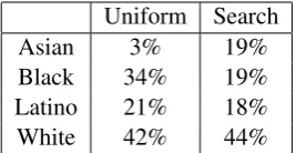
To investigate this, we used the Twitter Search API to collect profiles containing a predefined set of keywords indicating race. Examples include the terms “African”, “Black”, “Hispanic”, “Latin”, “Latino”, “Spanish”, “Chinese”, “Italian”, “Irish.” Profiles containing such words in the description field were collected. These were further filtered in an attempt to remove businesses (e.g., Chinese restaurants) by excluding profiles with the key-words in the name field as well as those whose name fields did not contain terms on the Census’ list of common first and last names. Remaining profiles were then manually reviewed for accu-racy. This resulted in 2,000 annotated users with the following distribution: Asian (377), Black (373), Latino (356), White (894). For each user, we collected their 200 most recent tweets using the Twitter API. We refer to this as theSearchdataset. Table 1 compares the race distribution for each of the two datasets. It is apparent that the Search dataset oversamples Asian users and undersam-ples Black users as compared to the Uniform dataset. This may in part due to the greater num-ber of keywords used to identify Asian users (e.g., Chinese, Japanese, Korean). This highlights the difficulty of obtaining a representative sample of Twitter users with the search approach, since the inclusion of a single keyword can result in a very different distribution of labels.

3.2 Models

3.2.1 County Regression

We build a text regression model to predict the racial makeup of a county (from the Census data)

Uniform Search

Asian 3% 19%

Black 34% 19%

Latino 21% 18%

White 42% 44%

Table 1: Percentage of users by race in the two validation datasets.

based on the linguistic patterns in tweets from that county. For each county, we create a feature vector as follows: for each unigram, we compute the pro-portion of users in the county who have used that unigram. We also distinguish between unigrams in the text of a tweet and a unigram in the description field of the user’s profile. Thus, two sample fea-ture values are (china, 0.1) and (desc china, 0.05), indicating that 10% of users in the county wrote a tweet containing the unigramchina, and 5% have the wordchinain their profile description. We ig-nore mentions and collapse URLs (replacing them with the token “http”), but retain hashtags.

We fit four separate ridge regression models, one per race.5 _{For each model, the independent}

variables are the unigram proportions from above; the dependent variable is the percentage of each county of a particular race. Ridge regression is an L2 regularized form of linear regression, where α determines the regularization strength, yi _{is a} vector of dependent variables for categoryi,Xis a matrix of independent variables, and β are the model parameters:

ˆ

βi_{= argmin} β ||y

i_−Xβi_||2

2+α||β||22

Thus, we have one parameter vector for each race category βˆ = {βˆA_,βˆB_,βˆL_,βˆW_{}. Related} ap-proaches have been used in prior work to estimate county demographics and health statistics (Eisen-stein et al., 2011; Schwartz et al., 2013b; Culotta, 2014).

the dot product between this binary feature vector xand the parameter vector for each category:

ˆ

y= argmax

i

x ·βˆi

3.2.2 Baseline 1: Logistic Regression

For comparison, we also train a logistic regres-sion classifier using the user-annotated data (either Uniform or Search). We perform 10-fold classifi-cation, using the same binary feature vectors de-scribed above (preliminary results using term fre-quency instead of binary vectors resulted in lower accuracy). We again use L2 regularization, con-trolled by tunable parameterα.

3.2.3 Baseline 2: Name Heuristic

Inspired by the approach of Chang et al. (2010), we collect Census data containing the frequency of racial categories by last name. We use the top 1000 most popular last names with their race dis-tribution from Census database. If the last name in the user’s Twitter profile matches names on this list, we categorize the user with the most probable race according to the Census data. For example, the Census indicates that 91% of peo-ple with the last name Garcia identify themselves as Latino/Hispanic. We would thus label Twit-ter users with Garcia as a last name as Hispanic. Users whose last names are not matched are cate-gorized as White (the most common label). 3.3 Experiments

We performed experiments to estimate the accu-racy of each approach, as well as how different training sets affect performance. The systems are: 1. County: The county regression approach of Section 3.2.1, trained only using county-level supervision.

2. Uniform: A logistic regression classifier trained on the Uniform dataset.

3. Search: A logistic regression classifier trained on the Search dataset.

4. Name heuristic: The name heuristic of Sec-tion 3.2.3.

We compare testing accuracy on both the Uni-form dataset and Search datasets. For experiments in which systems are trained and tested on the same dataset, we report the average results of 10-fold cross-validation.

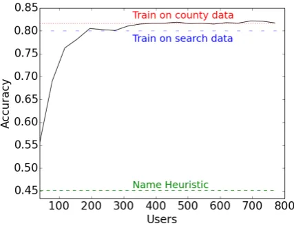
Figure 1: Learning curve for the Uniform dataset. The solid black line is the cross-validation accu-racy of a logistic regression classifier trained using increasingly more labeled examples.

Figure 2: Learning curve for the Search dataset. The solid black line is the cross-validation accu-racy of a logistic regression classifier trained using increasingly more labeled examples.

We tune theαregularization parameter for both ridge and logistic regression, reporting the best accuracy for each approach. Systems are imple-mented in Python using the scikit-learn li-brary (Pedregosa and others, 2011).

4 Results

PPP_PPP PPP

Train Test Search Uniform Search 0.7715 0.8000 Uniform 0.5535 0.8221 County 0.5490 0.8169 Name heuristic 0.4955 0.4519

Table 2: Accuracy of each system. PPP_PPP

PPP

Train Test Search Uniform Search 0.7650 0.8074 Uniform 0.4721 0.8130 County 0.4738 0.8050 Name heuristic 0.3838 0.3178

Table 3: F1 of each system.

be transferred to make inferences at the user level. Figure 1 also shows slightly lower accuracy from training on the Search dataset and testing on the Uniform dataset (80%). This may in part be due to the different label distributions between the datasets, as well as the different characteristics of the linguistic patterns, discussed more below.

The Name heuristic does poorly overall, mainly because few users provide their last names in their profiles, and only a fraction of those names are on the Census’ name list.

Figure 2 plots the learning curve for the Search dataset. Here, the County approach performs con-siderably worse than logistic regression trained on the Search data. However, the County approach again performs comparable to the supervised Uni-form approach. That is, training a supervised clas-sifier on the Uniform dataset is only slightly more accurate than training only using county supervi-sion (54.9% versus 55.3%). By F1, county super-vision does slightly better than the Uniform ap-proach. This again highlights the very different characteristics of the Uniform and Search datasets. Importantly, if we remove features from the user description field, then the cross-validation accu-racy of the Search classifier is reduced from 77% to 67%. Since a small set of keywords in the de-scription field were used to collect the Search data, the Search classifier simply recovers those key-words, thus inflating its performance.

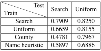
Tables 2-4 show the accuracy, F1, and precision for each method (averaged over each class label). The relative trends are the same for each metric. The primary difference is the high precision of the

PPP_PPP PPP

Train Test Search Uniform Search 0.7909 0.8250 Uniform 0.6659 0.8155 County 0.4781 0.7967 Name heuristic 0.5897 0.6886

Table 4: Precision of each system. PPP_PPP

PPP

Train Test County Search 0.0190 Uniform 0.0361 County 0.0186 Name heuristic 0.0154

Table 5: Mean Squared Error of each system on the task of predicting the racial makeup of a county. Values are averages over the four race cat-egories.

Name heuristic — when users do provide a last name on the Census list, this heuristic predicts the correct race 69% of the time on the Uniform data, and 59% of the time on the Search data.

We additionally compute how well the differ-ent approaches predict the county demographics. For the County method, we perform 10-fold cross-validation, using the original county feature vec-tors as independent variables. For the logistic re-gression methods, we train the classifier on one of the user datasets (Uniform or Search), then clas-sify each user in the county dataset. These pre-dictions are aggregated to compute the proportion of each race per county. For the name heuristic, we only consider users who match a name in the Census list, and use the heuristic to compute the proportion of users of each race.

Black White Latino Asian black white spanish asian african italian latin asian american irish hispanic filipino

black british spanish korean the french latino chinese

african german de korean

young girl en japanese

smh boy el philippines

to own que vietnamese

male italian latin japanese yall russian es filipino

niggas pretty la asians

woman fucking por japan

rip christmas latino chinese

man buying hispanic many

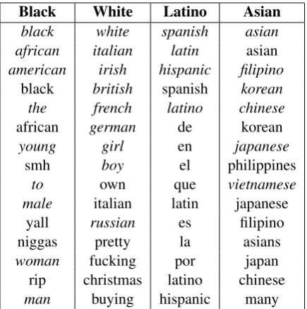
Table 6: Top-weighted features for the classifier trained on the Search dataset. Terms from the de-scription field are in italics.

though we do not investigate this here.

4.1 Analysis of top features

Tables 6-8 show the top 15 features for each sys-tem, sorted by their corresponding model parame-ters. In both our training and testing process, we distinguish between words in the user description field and words in tweets. We also include a fea-ture that indicates whether the user has any text at all in their profile description. In addition, we ig-nore mentions but retain hashtags. In these tables, words in description are shown in italics.

Because the Search dataset is collected by matching description keywords, in Table 6 many of these keywords are top-weighted features (e.g., ’black’, ’white’, ’spanish’, ’asian’). However in Table 7, there is no top feature word from the de-scription. This observation shows how our search dataset collection biases the resulting classifier.

The top features for the Uniform method (Ta-ble 7) tend to represent lexical variations and slang common among these groups. Interestingly, no terms from the profile description are strongly weighted, most likely a result of the uniform sam-pling approach, which does not bias the data to users with keywords in their profile.

For the County approach, it is less revealing to simply report the features with the highest weights. Since the regression models for each race were fit independently, many of the top-weighted

Black White Latino Asian

ain makes pizza were

lmao please 3rd sorry

somebody seriously drunk bit

tryna guys ti hahaha

bout whenever gets ma

nigga snow el hurts

niggas pretty estoy keep

black literally self team

smh thing lucky aw

tf isn special food

lil such everywhere sad

been am sleep packed

real red la care

everybody glass chicken goodbye

gon sucks tried forever

Table 7: Top-weighted features for the classifier trained on the Uniform dataset.

words are stop words (as opposed to the logistic regression approach, which treats this as a multi-class multi-classification problem). To report a more useful list of terms, we took the following steps: (1) we normalized the parameter vectors for each class by vector length; (2) from the parameter vec-tor of each class we subtracted the vecvec-tors of the other three classes (i.e.,βB_←βB_−(βA_+βL₊ βW_{)). The resulting vectors better reflect the} fea-tures weighted more highly in one class than oth-ers. We report the top 15 features per class.

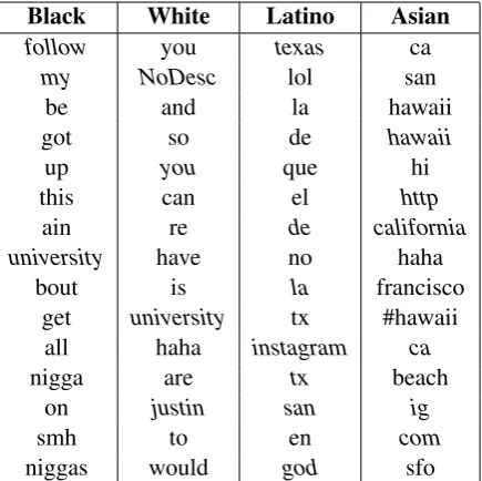
The top features for the County method (Ta-ble 8) reveal a mixture of lexical variations as well as geographical indicators, which act as prox-ies for race. There are many Spanish words for Latino-American users, for example ’de’, ’la’, and ’que.’ In addition there are some state names (’texas’, ’hawaii’), part of city names (’san’), and abbreviations (’sfo’ is the code for the San Fran-cisco airport). Texas is 37.6% Hispanic-American, and San Francisco is 34.2% Asian-American. Ref-erences to the photo-sharing site Instagram are found to be strongly indicative of Latino users. This is further supported by a survey conducted by the Pew Research Internet Project,6 _which

found that while an equal percentage of White and Latino online adults use Twitter (16%), online Latinos were almost twice as likely to use Insta-gram (23% versus 12%). Additionally, the term

6_{http://www.pewinternet.org/files/}

Black White Latino Asian

follow you texas ca

my NoDesc lol san

be and la hawaii

got so de hawaii

up you que hi

this can el http

ain re de california

university have no haha

bout is la francisco

get university tx #hawaii

all haha instagram ca

nigga are tx beach

on justin san ig

smh to en com

niggas would god sfo

Table 8: Top-weighted features for the regression model trained on the County dataset. Terms from the description field are in italics.

Truth Predicted Top Features

white latino de, la, que, no,la, el, san, en, amp, me

white black this, on, be, got, up, in, shit, at, the, all

black white you, and, to, you, the, is, so, of, have, re

Table 9: Misclassified by the County method.

“justin” in the user profile description is a strong indicator of White users – an inspection of the County dataset reveals that this is largely in ref-erence to the pop musician Justin Bieber. (Recall that users typically do not enter their own names in the description field.)

We find some similarities with the results of Eisenstein et al. (2011) — e.g., the term ’smh’ (“shaking my head”) is a highly-ranked term for African-Americans.

4.2 Error Analysis

We sample a number of users who were misclas-sified, then identify the highest weighted features (using the dot product of the feature vector and pa-rameter vector). Table 9 displays the top features of a sample of users in the Uniform dataset that were correctly classified by the Uniform method but misclassified by the County method. Similarly, Table 10 shows examples that were misclassified by the Uniform approach but correctly classified

Truth Predicted Top Features

black white makes, guys, thing, isn, am, again, haha, every-one, remember, very black white please, guys, snow, pretty,

literally, isn, am, again, happen, midnight

black white makes, snow, pretty, lit-erally, am, again, happen, yay, beer, amazing

Table 10: Misclassified by the classifier trained on the Uniform dataset.

by the County approach.

One common theme across all models is that be-cause White is the most common class label, many common terms are correlated with it (e.g., the, is, of). Thus, for users that use only very common terms, the models tend to select the White label. Indeed, examining the confusion matrix reveals that the most common type of error is to misclas-sify a non-White user as White.

5 Conclusions and Future Work

Our results suggest that models fit on aggregate, geolocated social media data can be used estimate individual user attributes. While further analysis is needed to test how this generalizes to other at-tributes, this approach may provide a low-cost way of inferring user attributes. This in turn will bene-fit growing attempts to use social media as a com-plement to traditional polling methods — by quan-tifying the bias in a sample of social media users, we can then adjust inferences using approaches such as survey weighting (Gelman, 2007).

There are clear ethical concerns with how such a capability might be used, particularly if it is ex-tended to estimate more sensitive user attributes (e.g., health status). Studies such as this may help elucidate what we reveal about ourselves through our language, intentionally or not.

References

F Al Zamal, W Liu, and D Ruths. 2012. Homophily and latent attribute inference: Inferring latent at-tributes of twitter users from neighbors. InICWSM.

Shlomo Argamon, Sushant Dhawle, Moshe Koppel, and James W. Pennebaker. 2005. Lexical predictors of personality type. In In proceedings of the Joint Annual Meeting of the Interface and the Classifica-tion Society of North America.

John D. Burger, John Henderson, George Kim, and Guido Zarrella. 2011. Discriminating gender on twitter. In Proceedings of the Conference on Em-pirical Methods in Natural Language Processing, EMNLP ’11, pages 1301–1309, Stroudsburg, PA, USA. Association for Computational Linguistics. Jonathan Chang, Itamar Rosenn, Lars Backstrom, and

Cameron Marlow. 2010. ePluribus: ethnicity on social networks. InFourth International AAAI Con-ference on Weblogs and Social Media.

Aron Culotta. 2014. Estimating county health statis-tics with twitter. InCHI.

Mark Dredze. 2012. How social media will change public health. IEEE Intelligent Systems, 27(4):81– 84.

Jacob Eisenstein, Noah A. Smith, and Eric P. Xing. 2011. Discovering sociolinguistic associations with structured sparsity. InProceedings of the 49th An-nual Meeting of the Association for Computational Linguistics: Human Language Technologies - Vol-ume 1, HLT ’11, pages 1365–1374, Stroudsburg, PA, USA. Association for Computational Linguistics.

George Forman. 2008. Quantifying counts and costs via classification. Data Min. Knowl. Discov., 17(2):164–206, October.

Kuzman Ganchev, Joo Graca, Jennifer Gillenwater, and Ben Taskar. 2010. Posterior regularization for struc-tured latent variable models. J. Mach. Learn. Res., 11:2001–2049, August.

Daniel Gayo-Avello. 2011. Don’t turn social media into another ’Literary digest’ poll. Commun. ACM, 54(10):121–128, October.

Andrew Gelman. 2007. Struggles with survey weight-ing and regression modelweight-ing. Statistical Science, 22(2):153–164.

Sharad Goel, Jake M Hofman, and M Irmak Sirer. 2012. Who does what on the web: A large-scale study of browsing behavior. InICWSM.

Shyam Gopinath, Jacquelyn S. Thomas, and Lakshman Krishnamurthi. 2014. Investigating the relationship between the content of online word of mouth, adver-tising, and brand performance. Marketing Science. Published online in Articles in Advance 10 Jan 2014.

Gary King. 1997. A solution to the ecological infer-ence problem: Reconstructing individual behavior from aggregate data. Princeton University Press.

Wendy Liu and Derek Ruths. 2013. What’s in a name? using first names as features for gender inference in twitter. In AAAI Spring Symposium on Analyzing Microtext.

Gideon S. Mann and Andrew McCallum. 2010. Generalized expectation criteria for semi-supervised learning with weakly labeled data. J. Mach. Learn. Res., 11:955–984, March.

Alan Mislove, Sune Lehmann, Yong-Yeol Ahn, Jukka-Pekka Onnela, and J. Niels Rosenquist. 2011. Un-derstanding the demographics of twitter users. In

Proceedings of the Fifth International AAAI Con-ference on Weblogs and Social Media (ICWSM’11), Barcelona, Spain.

Dong Nguyen, Noah A. Smith, and Carolyn P. Ros. 2011. Author age prediction from text using lin-ear regression. InProceedings of the 5th ACL-HLT Workshop on Language Technology for Cultural Heritage, Social Scie nces, and Humanities, LaT-eCH ’11, pages 115–123, Stroudsburg, PA, USA. Association for Computational Linguistics.

Brendan O’Connor, Ramnath Balasubramanyan, Bryan R. Routledge, and Noah A. Smith. 2010. From Tweets to polls: Linking text sentiment to public opinion time series. In International AAAI Conference on Weblogs and Social Media, Washington, D.C.

F. Pedregosa et al. 2011. Scikit-learn: Ma-chine learning in Python. Machine Learning Re-search, 12:2825–2830. http://dl.acm.org/

citation.cfm?id=2078195.

Marco Pennacchiotti and Ana-Maria Popescu. 2011. A machine learning approach to twitter user classifi-cation. In Lada A. Adamic, Ricardo A. Baeza-Yates, and Scott Counts, editors,ICWSM. The AAAI Press. Novi Quadrianto, Alex J. Smola, Tibrio S. Caetano, and Quoc V. Le. 2009. Estimating labels from label pro-portions. J. Mach. Learn. Res., 10:2349–2374, De-cember.

Delip Rao, David Yarowsky, Abhishek Shreevats, and Manaswi Gupta. 2010. Classifying latent user at-tributes in twitter. In Proceedings of the 2Nd In-ternational Workshop on Search and Mining User-generated Contents, SMUC ’10, pages 37–44, New York, NY, USA. ACM.

Delip Rao, Michael J. Paul, Clayton Fink, David Yarowsky, Timothy Oates, and Glen Coppersmith. 2011. Hierarchical bayesian models for latent at-tribute detection in social media. InICWSM. Sara Rosenthal and Kathleen McKeown. 2011. Age

online behavior in pre- and post-social media gen-erations. InProceedings of the 49th Annual Meet-ing of the Association for Computational LMeet-inguis- Linguis-tics: Human Language Technologies - Volume 1, HLT ’11, pages 763–772, Stroudsburg, PA, USA. Association for Computational Linguistics.

Jonathan Schler, Moshe Koppel, Shlomo Argamon, and James W Pennebaker. 2006. Effects of age and gender on blogging. InAAAI 2006 Spring Sym-posium on Computational Approaches to Analysing Weblogs (AAAI-CAAW), pages 06–03.

H Andrew Schwartz, Johannes C Eichstaedt, Mar-garet L Kern, Lukasz Dziurzynski, Stephanie M Ramones, Megha Agrawal, Achal Shah, Michal Kosinski, David Stillwell, Martin E P Seligman, and Lyle H Ungar. 2013a. Personality, gen-der, and age in the language of social media: the open-vocabulary approach. PloS one, 8(9):e73791. PMID: 24086296.