http://www.scirp.org/journal/ajcm ISSN Online: 2161-1211 ISSN Print: 2161-1203
DOI: 10.4236/ajcm.2017.73021 Aug. 17, 2017 243 American Journal of Computational Mathematics
Prediction of Better Flow Control Parameters
in MHD Flows Using a High Accuracy Finite
Difference Scheme
A. D. Abin Rejeesh1, S. Udhayakumar1, T. V. S. Sekhar2, R. Sivakumar1 1Department of Physics, Pondicherry University, Puducherry, India
2School of Basic Sciences, Indian Institute of Technology Bhubaneswar, Bhubaneswar, India
Abstract
We have successfully attempted to solve the equations of full-MHD model within the framework of ψ ω− formulation with an objective to evaluate the performance of a new higher order scheme to predict better values of control parameters of the flow. In particular for MHD flows, magnetic field and elec-trical conductivity are the control parameters. In this work, the results from our efficient high order accurate scheme are compared with the results of second order method and significant discrepancies are noted in separation length, drag coefficient and mean Nusselt number. The governing Navi-er-Stokes equation is fully nonlinear due to its coupling with Maxwell’s equa-tions. The momentum equation has several highly nonlinear body-force terms due to full-MHD model in cylindrical polar system. Our high accuracy results predict that a relatively lower magnetic field is sufficient to achieve full sup-pression of boundary layer and this is a favorable result for practical applica-tions. The present computational scheme predicts that a drag-coefficient
minimum can be achieved when β =0.4 which is much lower when
com-pared to the value β =1 as given by second order method. For a special val-ue of β =0.65, it is found that the heat transfer rate is independent of elec-trical conductivity of the fluid. From the numerical values of physical quanti-ties, we establish that the order of accuracy of the computed numerical results is fourth order accurate by using the method of divided differences.
Keywords
Full-MHD Equations, Forced Convective Heat Transfer, High Order Compact Schemes, Divided Differences
*Corresponding author. How to cite this paper: Abin Rejeesh,
A.D., Udhayakumar, S., Sekhar, T.V.S. and Sivakumar, R. (2017) Prediction of Better Flow Control Parameters in MHD Flows Using a High Accuracy Finite Difference Scheme. American Journal of Computa-tional Mathematics, 7, 243-275.
https://doi.org/10.4236/ajcm.2017.73021
Received: May 9, 2017 Accepted: August 14, 2017 Published: August 17, 2017
Copyright © 2017 by authors and Scientific Research Publishing Inc. This work is licensed under the Creative Commons Attribution-NonCommercial International License (CC BY-NC 4.0). http://creativecommons.org/licenses/by-nc/4.0/
DOI: 10.4236/ajcm.2017.73021 244 American Journal of Computational Mathematics
1. Introduction
The calculation and prediction of physical quantities to the desired accuracy is necessary in every engineering design because otherwise an under-performance together with an overshoot in the design cost. The study of magnetohydrodynamic flows with its heat transfer is important due to many practical applications in science and engineering. For instance, in many semiconducting single crystal growth processes, especially using the Czochralski technique, cylindrical shaped crystal is grown from the melt containing the material in the molten (liquid) state. In such systems, calculation of heat transfers is fairly complex due to the nonlinear coupling of the momentum with the heat diffusion and advection apart from radiative transfers. These semiconducting crystals are mostly used as substrates in electronic industry. However, during the crystal growth process, thermal stresses will be present if heat transfer is not well controlled [1]. Consequently, the resulting semiconducting single crystal substrates will have unavoidable dislocations which is an undesirable feature for applications. This means accurate calculation of the flow field, determination of temperature isotherms and hence precise estimates of heat transfer coefficients is of crucial importance in many practical applications. The accuracy of the final computed results from numerical simulation emerge from both the modeling (or approxi- mation methods) and also on the usage of a particular discretization method. In this paper, we address both the issues in order to have minimum approximation in modeling of physical system together with a highly accurate numerical solution by using a high order discretization procedure.
Many industrial applications include liquid metals in metallurgical processes such as stirring, pumping, casting, suppressing etc. [2]. The physical importance of the MHD flow is due to the coupling of Maxwell’s equations with momentum equation leading to mathematical complexity and fascinating physical phenomena such as flow acceleration or, suppression of flow, or modified heat transfer. The
magnetic Reynolds number Rm is an important physical parameter which
varies over several orders of magnitude depending on the nature of the system under consideration. For example, Rm is large in astrophysical and geophysical
flows while in metallurgical flow problems or in crystal growth processes, it is very small. Numerous theoretical, numerical and experimental studies have been carried out on MHD flows and bluff body flow dynamics. When an electrically conducting fluid moves through a magnetic field the fluid will experience a Lorentz force, leading to Joule dissipation that eventually reduces the kinetic energy of the fluid. That is, the velocity distribution is regenerated by the Lorentz force and suppress the turbulence in the wake region. The Lorentz force can reduce the drag force effectively and suppress the flow separation in fluid flows as evidenced by the following data.
DOI: 10.4236/ajcm.2017.73021 245 American Journal of Computational Mathematics the full solution in the entire domain of interest. In the case of boundary layer solution approach, the solutions are obtained within the boundary layer of the flow, and the detailed flow velocities and temperature will not be available in the domain of fluid flow. Under the first category a), limited attempts are made using Laplace transform technique [3] and perturbation techniques [4]. Under the second category b), the boundary layer solutions for different types of MHD flows and associated heat transfer has been studied by many authors [3][5]-[13], wherein the governing nonlinear partial differential equations are transformed to a set of ordinary differential equations and they are solved using Runge Kutta methods. In addition, many authors have used lower order accurate finite difference methods for the study of MHD flows and in particular with heat
transfer effects [14]. Various research groups target on different numerical
schemes in order to capture the flow and wake dynamics. One important feature to capture in the analysis is the Re at which separation starts. The orientation
of magnetic field direction (parallel/transverse) to the free stream velocity have different contribution to stabilize the flow [15] [16] which is also reported experimentally [17] [18]. The effect of magnetic field on the stabilization of unsteady flows has been studied by a linear stability analysis and concluded that the magnetic field can have both damping and enhancing influence on the instability of the flow [19][20]. In a recent experimental findings it is reported that the pressure drag coefficient can be increased with the help of magnetic field
[21]. The numerical studies on the effect of magnetic field on the flow around cylinder has been reported and where the accuracy will not exceed second order
[22][23] [24]. The MHD flow past circular cylinder has been studied using an
extension to immersed boundary method and concluded that the method is an efficient one to study the MHD problems [25]. Earth’s liquid core [26], liquids
involved in melting processes, crystal growth processing are some of the
branches where the low Prandtl number study is necessary
(
Pr1)
. Fluidsconnected with everyday lives such as water, oils, alcohols have the Pr~ 1
while molten alloys like GaInSn will have a Prandtl number of 0.022. The forced convective heat transfer studies due to power-law fluid flow past cylinder is
analyzed [27] and for the normal Newtonian fluid is analyzed [28] [29]. A
Lax-Wendroff type matrix distribution method is used and the numerical solution to the MHD flow with heat transfer is studied [30] and concluded that the method is robust and accurate, where a combination of second order and third-order upwind schemes were used. In addition to change of drag coefficient due to magnetic field, experimental studies revealed that heat transfer rate can be reduced using applied magnetic field [31][32]. Without magnetic field effects, the forced convection heat transfer from circular cylinder due to air and liquids has been analyzed experimentally and the data is correlated with Pr and Re
[33]. It is also reported experimentally that an applied magnetic field will
DOI: 10.4236/ajcm.2017.73021 246 American Journal of Computational Mathematics presence of magnetic field has been analyzed experimentally [35][36] and later numerically using a spectral method and observed that the applied magnetic field will reduce the oscillating amplitude of lift coefficients [37]. The study of liquid metal flow past a cylinder inside a duct provided means of understanding the effect of magnetic field on Re and found that the imposed magnetic field
will shift the appearance of flow instabilities to higher Re [38]. There are a few
reports on the use of high order numerical schemes in curvilinear systems. The problem of flow past impulsively started cylinder is analyzed using a semi- compact high order scheme and concluded that the scheme is capable of
capturing the physical phenomena [39]. The classical problem of flow past
cylinder (without external magnetic field) has been studied using a high order finite difference scheme wherein it is reported that the numerical scheme at a fairly coarser grid is sufficient to get accurate results [40]. In the present work we develop a new fourth order accurate discretization scheme for the full-MHD model in the streamfunction-vorticity formulation in cylindrical polar coordinate system and the effectiveness of the scheme is tested in terms of predicting better
control parameters in the MHD flows. The computed velocities from ψ and
ω will be having higher numerical accuracy. Experimental measurement of
velocities of the fluids of MHD flows with magnetic field can be found in the literature [41].
2. Governing Equations for MHD Flows
In order to study the steady state flow properties and heat transfer in flows of electrically conducting fluids in presence of magnetic field, the governing equations would be the modified Navier-Stokes equation (in which additional body force terms due to magnetic field) which is coupled with the Maxwells equations of electrodynamics together with energy equation. The non- dimensionalized equations under consideration are
0
∇ ⋅ =q (1)
(
)
2 2(
)
p
Re β
⋅∇ = −∇ + ∇ + ×
q q q j H
(2)
0
∇ ⋅H = (3)
t
∂ ∇ × = +
∂
D
H j
(4)
0
∇ ⋅ =j (5)
(
)
2
m
R
= + ×
j E q H
(6)
(
)
2 2T T
RePr
⋅∇ = ∇
q
(7)
where the following definitions are used in the process of non-dimensionalization.
2
'
, , , ,
s
T T
q p r
q p r T
U ρU a T T
∞
∞ ∞ ∞
′
′ ′ −
= = = =
DOI: 10.4236/ajcm.2017.73021 247 American Journal of Computational Mathematics
, ,
H E j
H E j
H∞ E∞ j∞
′ ′ ′
= = =
in which the primed variables denote the respective quantities with dimensions.
The Alfvén number β is a dimensionless quantity characterizing the flow in
presence of magnetic field and it is the ratio of the speed of the Alfvén wave to the speed of the main stream fluid. The last term in Equation (2) is the body force term which is nonlinearly coupled with other equations in the list. Equation (1) is due to incompressibility condition while Equations ((3) and (4)) are the Maxwell’s equations to be satisfied for the applied magnetic field H. In
the Amperes law (4), the second term is due to electric displacement vector D.
Since displacement current density is negligible in fluid flows the second term in the right hand side of Equation (4) can be dropped. For steady state conditions, the electrodynamic continuity equation is (5) and the conduction current density j has to satisfy the Ohms law which is Equation (6). First it is noted
that Equations ((1) to (6)) are coupled. Now, if heat transfer analysis is to be carried out, then the energy transport equation to be solved is given by Equation (7). If we solve (7) by treating the velocity q as coupled with Equations ((1) to
(6)) then we can get the natural convection heat transfer properties. On the other hand, if we first solve the set of Equations ((1) to (6)) and provide this solution to Equation (7) as its input, then we can study the forced convection properties. In any case, first we need a discretization scheme to solve the governing equations. In the following, we propose to device a solution method based on streamfunction-vorticity approach and which is suitable for two- dimensional flow simulations. In cylindrical polar system, the velocity and applied magnetic field are
(
q qr, θ, 0)
=
q (8)
(
h hr, θ, 0)
=
H (9)
To satisfy the incompressibility condition, the velocity components can be expressed in terms of a scalar streamfunction ψ given by
( )
1( )
, ,r
r q r
r
ψ θ
θ
θ
∂ = ⋅
∂ (10)
( )
,( )
r,q r
r
θ
ψ θ
θ = −∂
∂ (11)
Since Equations ((1) and (3)) exhibit solenoidal nature, a definition similar to (10) and (11) can be used by making use a scalar called magnetic streamfunction, denoted by A as below.
( )
1( )
, ,r
A r h r
r
θ θ
θ
∂ = ⋅
∂ (12)
( )
, A r( )
,h r
r
θ
θ
θ = −∂
∂ (13)
DOI: 10.4236/ajcm.2017.73021 248 American Journal of Computational Mathematics × =q
∇ ω (14)
which, upon using (10) and (11), we get the differential equation for velocity as below.
1 r
q q q
r r r
θ θ ω
θ
∂ ∂
+ − =
∂ ∂ (15)
and where ω has components only in the z-direction and is a function of r
and θ of the cylindrical polar coordinate system. We make use of Equation (14) in (2) by applying the curl operator to (2) which results in
(
)
2(
)
{
}
Re β
− × ×∇ q ω = − ⋅ ×∇ ∇×ω + ⋅∇ ∇× ×H ×H
(16) where we have also used (4) after neglecting the displacement vector. In the present work, we consider the case of applying only an external magnetic field but no electric field is applied. In addition, for the case of two-dimensional flows, it can be shown that E=0 if only magnetic field is applied to the electrically
conducting flow. Then, from (4) and (6), we have
(
)
2
m
R
×H= ⋅ ×q H
∇
(17)
Using (17) in (16) and then expanding the curl operator in the cylindrical system and by making use of (9) we obtain the differential equation for vorticity as given below.
2 2
2 2
2
2
2 1 1
2 2
2
r
m r r r r
r r
r
r r
r r r r
q q
r r Re r r r r
R h q h q h h q
h q h
r r r r
h h q h
h q
h q h q h h
r r r r
θ
θ θ θ
θ
θ θ θ
θ θ
ω ω ω ω ω
θ θ β θ ∂ + ∂ − ∂ + ∂ + ∂ ∂ ∂ ∂ ∂ ∂ ∂ ∂ = ⋅ − − − + ∂ ∂ ∂ ∂ ∂ ∂ + + + + ∂ ∂ ∂ ∂ 2 r r r r
h q h h q h h q h h
r r r r
θ θ θ θ θ θ
θ θ θ θ
∂ ∂ ∂ ∂ + − − − ∂ ∂ ∂ ∂ (18)
Now, if we simplify the Equation (17) using (8) and (9) we get the differential equation for magnetic field as follows.
(
)
1
2
m r r r R q h q h
h h h
r r r
θ θ θ θ θ − ∂ ∂ + − ⋅ =
∂ ∂ (19)
Similarly, Equation (7) is simplified using (10) and (11) to yield the differential equation for temperature as given below.
2 2
2 2 2
2 1 1
r
T T T T T
q q
r θ θ Re Pr r r r r θ
∂ ∂ ∂ ∂ ∂
+ = + +
∂ ∂ ⋅ ∂ ∂ ∂
(20)
Finally we have a set of four coupled partial differential Equations ((15), (18)-(20)) having several nonlinear terms in the vorticity differential equation.
The components of q and H appearing in these four equations are given by
DOI: 10.4236/ajcm.2017.73021 249 American Journal of Computational Mathematics cylindrical geometry.
3. Discretization Procedure
In this section we outline the discretization procedure for the discretization of governing equations. The implementation of fourth order finite differences to the governing equations for the present problem requires considerable exercise because of curvilinear coordinate system. From the Taylor series, for the ξ and
η-direction, if we denote h and k as the grid spacing along radial and angular
direction then, the fourth order accurate finite differences for the first and second derivatives can be written as
( )
2 3 4 3 6 hDξ h
ξ ξ
∂Ψ= Ψ − ∂ Ψ+
∂ ∂
(21)
( )
2 2 4
2 4
2 4
12
h
Dξ h
ξ ξ
∂ Ψ ∂ Ψ
= Ψ − +
∂ ∂ (22)
( )
2 3 4 3 6 kDη k
η η
∂Ψ= Ψ − ∂ Ψ+
∂ ∂ (23)
( )
2 2 4
2 4
2 4
12
h
Dη k
η η
∂ Ψ ∂ Ψ
= Ψ − +
∂ ∂
(24)
where Dξ , Dξ2, Dη and Dη2 denote the standard second order central
difference operators which are given by
1, 1,
,
2
i j i j i j
D
h
ξ
+ −
Ψ − Ψ
Ψ =
(25)
1, , 1,
2
, 2
2
i j i j i j i j
D
h
ξ
+ −
Ψ − Ψ + Ψ
Ψ =
(26)
, 1 , 1 ,
2
i j i j i j
D
k
η
+ −
Ψ − Ψ
Ψ =
(27)
, 1 , , 1
2
, 2
2
i j i j i j i j
D
k
η
+ −
Ψ − Ψ + Ψ
Ψ =
(28)
The second order central difference operators for cross-derivatives can be obtained from Taylor series, and are given by
, 1, 1 1, 1 1, 1 1, 1
1 4
i j i j i j i j i j
D D
hk
ξ ηΨ = Ψ+ + − Ψ+ − − Ψ− + + Ψ− −
(29)
(
)
2
, 2 1, 1 1, 1 1, 1 1, 1 , 1 , 1
1
2 2
i j i j i j i j i j i j i j
D D
h k
ξ ηΨ = Ψ+ + − Ψ+ − + Ψ− + − Ψ− − − Ψ + − Ψ − (30)
(
)
2
, 2 1, 1 1, 1 1, 1 1, 1 1, 1,
1
2 2
i j i j i j i j i j i j i j
D D
hk
ξ ηΨ = Ψ+ + + Ψ+ − − Ψ− + − Ψ− − − Ψ+ − Ψ− (31)
(
)
2 2
, 2 2 1, 1 1, 1 1, 1 1, 1
1, 1, , 1 , 1 ,
1
2 4
i j i j i j i j i j
i j i j i j i j i j
D D
h k
ξ η + + + − − + − −
+ − + −
Ψ = Ψ + Ψ + Ψ + Ψ
− Ψ + Ψ + Ψ + Ψ + Ψ
DOI: 10.4236/ajcm.2017.73021 250 American Journal of Computational Mathematics 3.1. Discretization of Streamfunction Equation
Equation (15) along with definitions (10) and (11) gives
1 1 1
r r r r r r
ψ ψ ψ ω
θ θ ∂ ∂ ∂ ∂ ∂ + − = ∂ ∂ ∂ ∂ ∂
(33)
Now the transformation r=eπξ and θ=πη are implemented followed y
the usage of D-operator from Equations ((21) to (28)) so that the above equation becomes.
(
)
2 4 2 4
2 2 4 4
, , , 4 4
,
,
12 12
i j i j i j
i j
h k
Dξ Dη s h k
ψ ψ ψ ψ ξ η ∂ ∂ + + = + + ∂ ∂
(34)
where the RHS of the above equation is the truncation error term and
(
4 4)
,
h k
indicates that the above equation is of the order of 4
h in ξ direction and of the order of 4
k in η direction. and
2 2π
, π e ,
i j i j
s = ξω
(35)
Since the Equation (34) inherently contain higher order derivatives of the stream function, they are computed as
3 3
2
3 2
s
D Dξ η D sξ
ψ ψ ψ
ξ
ξ ξ η
∂ = − ∂ − ∂ = − −
∂
∂ ∂ ∂ (36)
4 4 2
2 2 2
4 2 2 2
s
D Dξ η D sξ
ψ ψ ψ
ξ ξ η ξ
∂ = − ∂ −∂ = − −
∂ ∂ ∂ ∂ (37)
3 3
2
3 2
s
D Dξ η D sη
ψ ψ ψ
η
η ξ η
∂ ∂ ∂
= − − = − −
∂
∂ ∂ ∂ (38)
4 4 2
2 2 2
4 2 2 2
s
D Dξ η D sη
ψ ψ ψ
η ξ η η
∂ ∂ ∂
= − − = − −
∂ ∂ ∂ ∂ (39)
Substituting Equations (36)-(39) in the discretized streamfunction Equation (34) and applying the D-operator from Equations (25)-(32), we get the fourth order accurate discretized representation of Equation (33) as given below.
(
)
(
)
(
)
(
)
(
)
(
)
[ ]
(
)
[ ]
{
}
8
2 2 2 2
0 1 3 2 4
5
2 2 2 2π 2 2 2
0
2 2 2 2
π e 1 4π 4π
i i
z h k k z h z z
h k ξ x x Dξ xDξ yDη
ψ ψ ψ ψ ψ ψ
ω ω ω
= − − + − + + − + + = − + + + +
∑
(40)where x=h2 12, y=k2 12 and
z= +x y,
8 0 i i ψ =
∑
represents the 8 nearestneighboring points and a centre point in the computational domain.
3.2. Discretization of Vorticity Equation
Equation (18) is simplified using Equations (10)-(13) and then r=eπξ with
π
θ= η is applied. Then, we can arrive at the following equation in terms of ξ and η.
2 2
2 2 c d F
ω ω ω ω
ξ η
ξ η
∂ +∂ + ∂ + ∂ =
∂ ∂
∂ ∂ (41)
DOI: 10.4236/ajcm.2017.73021 251 American Journal of Computational Mathematics 2 Re c ψ η ∂ = − ∂
(42)
2 Re d ψ ξ ∂ = ∂
(43)
and
2π 2 2
2 2 2
2 2 2
2 2 2 2 2
2 2 e 2 4π 2 2π m
A A A A A A
F Re R
A A A A A A
A A A
ξ ψ ψ ψ
β π
η η ξ ξ ξ η η η ξ
ψ ψ ψ
ξ η ξ η ξ η ξ η ξ η ξ η
ψ ψ ψ
ξ η η ξ ξ η
− − ∂ ∂ ∂ ∂ ∂ ∂ ∂ ∂ ∂ = ⋅ ⋅ ∂ ∂− − + ∂ ∂ ∂ ∂ ∂ ∂ ∂ ∂ ∂ ∂ ∂ ∂ ∂ ∂ ∂ ∂ + + − ∂ ∂ ∂ ∂ ∂ ∂ ∂ ∂ ∂ ∂ ∂ ∂ ∂ ∂ ∂ ∂ ∂ ∂ − + + ∂ ∂ ∂ ∂ ∂ ∂ (44)
On substitution of Equations (21)-(24) in the vorticity Equation (41) we get the discretized form as below.
2 2
, , , , , , , ,
i j i j i j i j i j i j i j i j
Dξω +Dηω +c Dξω +d Dηω +τ =F
(45) and the truncation error τ in (45) is
(
)
2 3 2 4 2 3 2 4
4 4
, 3 4 3 4
,
,
6 12 6 12
i j
i j
h h k k
c ω ω d ω ω h k
τ
ξ ξ η η
∂ ∂ ∂ ∂
= − + + + +
∂ ∂ ∂ ∂
(46)
Now, to eliminate the third and fourth derivatives of ω that are present in
the truncation error term, we differentiate (41) once and twice with respect to ξ and η respectively, to yield the following.
3 3 2 2
3 2 2
c d F
c d
ω ω ω ω ω ω
ξ η ξ ξ ξ η ξ
ξ ξ η ξ
∂ ∂ ∂ ∂ ∂ ∂ ∂ ∂ ∂
= − − − − − −
∂ ∂ ∂ ∂ ∂ ∂ ∂
∂ ∂ ∂ ∂ (47)
4 4 3 3 2
2
4 2 2 2 2 2
2 2 2 2 2 2 2 2 2 c
c d c
d c c
cd c
d d F F
c c
ω ω ω ω ω
ξ
ξ ξ η ξ η ξ η ξ
ω ω
ξ ξ η ξ ξ ξ
ω
ξ ξ η ξ ξ
∂ = − ∂ + ∂ − ∂ + − ∂ ∂ ∂ ∂ ∂ ∂ ∂ ∂ ∂ ∂ ∂ ∂ ∂ ∂ ∂ ∂ + − + − ∂ ∂ ∂ ∂ ∂ ∂ ∂ ∂ ∂ ∂ ∂ + − + − ∂ ∂ ∂ ∂ ∂ (48)
3 3 2 2
3 2 2
c d F
c d
ω ω ω ω ω ω
ξ η η ξ η η η
η ξ η η
∂ ∂ ∂ ∂ ∂ ∂ ∂ ∂ ∂
= − − − − − −
∂ ∂ ∂ ∂ ∂ ∂ ∂
∂ ∂ ∂ ∂
(49)
4 4 3 3 2
4 2 2 2 2
2 2 2 2 2 2 2 2 2 2 2 c
c d cd
d c c
d d
d d F F
d d
ω ω ω ω ω
η ξ η
η ξ η ξ η ξ η
ω ω
η η η η ξ
ω
η η η η η
∂ = − ∂ − ∂ + ∂ + − ∂ ∂ ∂ ∂ ∂ ∂ ∂ ∂ ∂ ∂ ∂ ∂ ∂ ∂ ∂ ∂ ∂ + − + − ∂ ∂ ∂ ∂ ∂ ∂ ∂ ∂ ∂ ∂ + − + − ∂ ∂ ∂ ∂ ∂ (50)
DOI: 10.4236/ajcm.2017.73021 252 American Journal of Computational Mathematics accurate representation of vorticity Equation (41) as below.
(
)
(
)
(
)
(
)
(
)
(
)
(
)
(
)
(
)
2 2 2 2
0 1
2 2 2 2
2 3
2 2
4 5
6 7
8
2 2 2π
2
8 2 4 2 8 4
4 2 8 4 4 2 8 4
4 2 8 4 4 2 2
4 2 2 4 2 2
4 2 2
e π
m
ek fh z k e hk g z hzc
h f h ko z kzd k e hk g z hzc
h f h ko z kzd z hcz kdz hkl
z hcz kdz hkl z hcz kdz hkl
z hcz kdz hkl
h k ReR
G xc D y
ξ
ξ
ω ω
ω ω
ω ω
ω ω
ω β −
− + − + + − −
+ + − − + − − +
+ − − + + + + +
+ − + − + − − +
+ + − −
−
=
{
+(
+)
(
2 2)
[ ]
}
[ ]
d Dη G + xDξ +yDη G
(51)
where
[ ]
[ ]
[ ]
[ ]
[ ]
[ ]
[ ] [ ]
[ ]
[ ] [ ]
[ ]
[ ] [ ]
[ ]
[ ] [ ] [ ]
[ ] [ ] [ ]
[ ] [ ] [ ]
2 2
2 2
2π
2 2π
G D D D A D D D A D D D A
D A D D D A D D A D D A
D A D A D D D D A D A
D A D A D D A D A D
η η ξ ξ ξ η η η ξ
ξ η ξ η ξ η ξ η
ξ η ξ η ξ η η
η η ξ ξ ξ η
ψ ψ ψ
ψ ψ
ψ ψ
ψ ψ
= − − +
+ +
− −
+ +
(52)
where the values of ψ around ψi j, are indexed as shown in the 2D compact stencil (Figure 1). Further, the coefficients required in the above equations are as follows.
[ ]
{
2}
1
e= +x c −ReD Dξ η ψ (53)
[ ]
{
2}
1
f = +y d +ReD Dξ η ψ
[image:10.595.209.541.358.706.2](54)
DOI: 10.4236/ajcm.2017.73021 253 American Journal of Computational Mathematics
{
2 2}
[ ]
π e2 2π[ ]
2
Re
g=− Dη +yd Dη +xc D Dξ η+z D Dξ η ψ +y ξDη ω
(55)
{
2 2}
[ ]
π e2 2π[ ]
2
Re
o= Dξ +xc Dξ +yd D Dξ η +z D Dξ η ψ +x ξDξ ω
(56)
{
2 2}
[ ]
l=zcd+Re x Dξ −y Dη ψ
(57) In addition to the above, we ill represent Equations ((42) and (43)) in fourth order accurate discrete form as below
[ ]
2[ ]
2 2π[ ]
1π e 2
c= −Re Dη ψ +y D Dξ η ψ +y ξDη ω
(58)
[ ]
2[ ]
2 2π[ ]
1π e 2
d=Re Dξ ψ +xD Dξ η ψ +x ξDξ ω
(59)
3.3. Discretization of Magnetic Streamfunction
Similar to the case of streamfunction equation, first the equation for magnetic field (19) is expressed in terms of magnetic stream function using Equations ((12) and (13)) and the velocities are replaced using (10) and (11), so that we get the magnetic streamfunction equation as given below
2 2
2 2 0
A A A A
C D ξ η ξ η ∂ ∂ ∂ ∂ + + + = ∂ ∂
∂ ∂
(60)
where the coefficients C and D are
2 m R C ψ η ∂ = − ∂
(61)
2 m R D ψ ξ ∂ = ∂
(62)
Substituting (21)-(24) in the magnetic streamfunction Equation (60), we get
2 2
, , , , , , , 0
i j i j i j i j i j i j i j
D Aξ +D Aη +C D Aξ +D D Aη +ζ =
(63) and the truncation error in the Equation (63) is
(
)
2 3 2 4 2 3 2 4
4 4
, 3 4 3 4
,
,
6 12 6 12
i j
i j
h A h A k A k A
C D h k
ζ
ξ ξ η η
∂ ∂ ∂ ∂
= − + + + +
∂ ∂ ∂ ∂
(64)
It may be noted that the coefficients in the magnetic streamfunction equations are denoted by C and D while those in vorticity equation are denoted by c and d. Also, the coefficient D in the above equation may not confuse with the operators like Dξ because operators will always have a suffix ξ or η. Elimination of
higher order derivatives of A in (64) is done by differentiating the magnetic
streamfunction Equation (60) once and twice with respect to ξ and η
respectively, to yield the following.
3 3 2 2
3 2 2
A A A A C A D A
C D
ξ η ξ ξ ξ η
ξ ξ η ξ
∂ ∂ ∂ ∂ ∂ ∂ ∂ ∂
= − − − − −
∂ ∂ ∂ ∂ ∂ ∂
DOI: 10.4236/ajcm.2017.73021 254 American Journal of Computational Mathematics
4 4 3 3 2
2
4 2 2 2 2 2
2 2 2
2 2
= 2
2
A A A A C A
C D C
D A C C A D D A
CD C C
ξ
ξ ξ η ξ η ξ η ξ
ξ ξ η ξ ξ ξ ξ ξ η
∂ ∂ ∂ ∂ ∂ ∂ − + − + − ∂ ∂ ∂ ∂ ∂ ∂ ∂ ∂ ∂ ∂ ∂ ∂ ∂ ∂ ∂ ∂ ∂ + − + − + − ∂ ∂ ∂ ∂ ∂ ∂ ∂ ∂ ∂ (66)
3 3 2 2
3 2 2
A A A A C A D A
C D
ξ η η ξ η η
η ξ η η
∂ ∂ ∂ ∂ ∂ ∂ ∂ ∂
= − − − − −
∂ ∂ ∂ ∂ ∂ ∂
∂ ∂ ∂ ∂ (67)
4 4 3 3 2
4 2 2 2 2
2 2 2
2
2 2 2
= 2
2
A A A A C A
C D CD
D A C C A D D A
D D D
η ξ η
η ξ η ξ η ξ η
η η η η ξ η η η
∂ − ∂ − ∂ + ∂ + − ∂ ∂ ∂ ∂ ∂ ∂ ∂ ∂ ∂ ∂ ∂ ∂ ∂ ∂ ∂ ∂ ∂ ∂ ∂ ∂ + − + − + − ∂ ∂ ∂ ∂ ∂ ∂ ∂ ∂
(68)
Now we first substitute (61)-(68) in Equation (63) and then apply D-operators from Equations (25)-(32) to arrive at the fourth order accurate discretized representation of the magnetic streamfunction Equation (60) as given below.
(
)
2 2
2 2 2 2 0
D D D D D D A
x y D D C D D DD D A
ξ η ξ η ξ η
ξ η ξ η ξ η
α β γ λ µ
− − ′ + + + − + − − = (69)
where the coefficients α, β′, γ, λ, µ, C and D appearing above are
given by
(
2)
1 xC R x D Dm ξ η
α = + − ψ
(70)
(
2)
21 yD R yDm η
β′ = + − ψ
(71)
2 2 2
2 2π 2 2 π e 2 m m m R R
C x D D C D D y D D D D
R
y d
ξ η ξ η ξ η η
ξ η
γ ψ ψ
ω = + − − − − (72)
(
)
2 2 2
2 2π
2 2
π e 2π 2
m m
m
R R
D x D D C D y D D D D D
R
x D
ξ η ξ ξ η ξ η
ξ
ξ
λ ψ ψ
ω = + + − + + + (73)
(
)
2 2 mR xDξ yDη x y C D
µ= − + ψ − +
(74)
In addition to the above, we ill represent Equations ((61) and (62)) in fourth order accurate discrete form as below
2 2 2π
2 π e
2
m
m
R
C= Dη+ yD Dξ ηψ +R y ξDηω
(75)
(
)
2 2 2π
2 π e 2
2
m
m
R
D= − Dξ + xD Dξ ηψ−R x ξ π+Dξ ω
(76)
3.4. Discretization of Energy Equation
In Equation (20) velocities are eliminated using (10) and (11) then, π
e
r= ξ and π
DOI: 10.4236/ajcm.2017.73021 255 American Journal of Computational Mathematics
2 2
2 2 0
T T T T
c d ξ η ξ η ∂ ∂ ′∂ ′∂ + + + = ∂ ∂
∂ ∂ (77)
where the coefficients, c′ and d′ are given by
2 RePr c ψ η ∂ ′ = − ∂
(78)
2 RePr d ψ ξ ∂ ′ = ∂
(79)
Equations (21)-(24) are applied on the above equation so that we have
2 2
, , , , , , , 0
i j i j i j i j i j i j i j
D Tξ +D Tη +c D T′ ξ +d D T′ η +γ =
(80)
The truncation error in the Equation (80) is
(
)
2 3 2 4 2 3 2 4
4 4
, 3 4 3 4 ,
6 12 6 12
i j
h T h T k T k T
c d h k
γ
ξ ξ η η
′ ∂ ∂ ′ ∂ ∂
= − + + + +
∂ ∂ ∂ ∂
(81)
In order to higher derivatives of T present in the truncation error terms, we differentiate the energy Equation (77) once and twice with respect to ξ and η
respectively and we get the following
3 3 2 2
3 2 2
T T T T c T d T
c d
ξ η ξ ξ ξ η
ξ ξ η ξ
′ ′
∂ = − ∂ − ′∂ − ′ ∂ −∂ ∂ −∂ ∂
∂ ∂ ∂ ∂ ∂ ∂
∂ ∂ ∂ ∂ (82)
4 4 3 3 2
2
4 2 2 2 2 2
2 2 2
2 2
2
2
T T T T c T
c d c
d T c c T d d T
c d c c
ξ
ξ ξ η ξ η ξ η ξ
ξ ξ η ξ ξ ξ ξ ξ η
′ ∂ = − ∂ + ′ ∂ − ′ ∂ + ′ − ∂ ∂ ∂ ∂ ∂ ∂ ∂ ∂ ∂ ∂ ∂ ′ ′ ′ ′ ′ ′ ′ ∂ ∂ ′∂ ∂ ∂ ′∂ ∂ ∂ + − + − + − ∂ ∂ ∂ ∂ ∂ ∂ ∂ ∂ ∂ (83)
3 3 2 2
3 2 2
T T T T c T d T
c d
ξ η η ξ η η
η ξ η η
′ ′
∂ = − ∂ − ′ ∂ − ′∂ −∂ ∂ −∂ ∂
∂ ∂ ∂ ∂ ∂ ∂
∂ ∂ ∂ ∂ (84)
4 4 3 3 2
2
4 2 2 2 2 2
2 2 2
2 2
2
2
T T T T d T
c d d
c T c c T d d T
c d d d
η
η ξ η ξ η ξ η η
η ξ η η η ξ η η η
′ ∂ ∂ ′ ∂ ′ ∂ ′ ∂ ∂ = − − + + − ∂ ∂ ∂ ∂ ∂ ∂ ∂ ∂ ∂ ′ ′ ′ ′ ′ ′ ′ ∂ ∂ ′∂ ∂ ∂ ′∂ ∂ ∂ + − + − + − ∂ ∂ ∂ ∂ ∂ ∂ ∂ ∂ ∂ (85)
Now substituting Equations (78)-(85) in the truncation error terms of Equation (77), and applying operator D to the derivatives, we will get the fourth order discretized form of energy equation, as given below
(
)
2 2
2 2 2 2 0
D D D D D D T
x y D D C D D DD D T
ξ η ξ η ξ η
ξ η ξ η ξ η
ς ρ ϖ ϑ ε
− − + + + − + − − =
(86)
where the coefficients ς, ρ, ϖ , ϑ, ε, c′ and d′ appearing above are
given by
(
2)
1 xc RePr x D Dξ η
ς= + ′ − ψ
(87)
(
2)
21 yd RePr y Dη
ρ= + ′ − ψ
DOI: 10.4236/ajcm.2017.73021 256 American Journal of Computational Mathematics
2 2 2
2 2π
2 2
π e 2
RePr RePr
c x D D c D D y D D d D
RePr
y d
ξ η ξ η ξ η η
ξ η
ϖ ψ ψ
ω ′ ′ ′ = + − − − − (89)
(
)
2 2 2
2 2π
2 2
π e 2π 2
RePr RePr
d x D D c D y D D d D D
RePr
x D
ξ η ξ ξ η ξ η
ξ
ξ
ϑ ψ ψ
ω ′ ′ ′ = + + − + + + (90)
(
)
2 2RePr xDξ yDη x y c d
ε= − + ψ− + ′ ′
(91)
In addition to the above, we will represent Equations ((78) and (79)) in fourth order accurate discrete form as below
2 2 2π
2 π e
2
RePr
c′ = Dη+ yD Dξ ηψ +RePr y ξDηω
(92)
(
)
2 2 2π
2 π e 2π
2
RePr
d′ = − Dξ + xD Dξ ηψ −RePr x ξ +Dξ ω
(93)
3.5. Boundary Conditions and Implementation
We evaluate the performance of the above discretization scheme by running numerical experiments for the MHD flow around a cylinder, since it is one of the classic problems in MHD flow where the flow features have been studied by many authors. Hence we can compare our high accuracy results and discuss on the performance of proposed discretization scheme. In order to cluster more grid points near the surface of the cylinder, an exponential transformation is employed. It is also assumed that the magnetic field will not penetrate across the boundary of the cylinder. The boundary conditions used are the following. On the surface of the cylinder, ψ =0, ∂ψ ∂ =r 0, ω= ∂2ψ ∂r2 and A=0. Far
away from the cylinder which is denoted by ξ → ∞, the imposed conditions are
( )
~ sinrψ θ , ω→0, A→rsin
( )
θ . The axis of symmetry is given by η =0and η =1, on which lines, the boundary conditions imposed are ψ =0, ω=0,
and A=0. For solving the energy equation, we impose a uniform temperature
1
T= on the cylinder surface and T =0 at far-field distances. On the axis of
symmetry, ∂ ∂ =T η 0 is imposed. The derivatives appearing in the boundary
conditions for streamfunction vorticity and temperature are
0
ψ ξ
∂ =
∂ (94)
2 2 2 2 π ψ ω ξ ∂ = −
∂ (95)
0
T η
∂ =
∂ (96)
DOI: 10.4236/ajcm.2017.73021 257 American Journal of Computational Mathematics
(
2, 3, 4, 5,)
1,
48 36 16 3
25
j j j j
j
ψ ψ ψ ψ
ψ = − + −
(97)
(
, 1, 2, 3,)
1,
48 36 16 3
25
n j n j n j n j
n j
ψ ψ ψ ψ
ψ − − −
+
− − + −
=
(98)
(
,2 ,3 ,4 ,5)
,1
48 36 16 3
25
i i i i
i
T T T T
T = − + −
(99)
(
, , 1 , 2 , 3)
, 1
48 36 16 3
25
i m i m i m i m
i m
T T T T
T + =− − − + − − −
(100)
The vorticity boundary condition used on the surface of the cylinder is the Briley’s formula
(
2, 3, 4,)
1, 2
108 27 4
18
j j j
j
h
ψ ψ ψ
ω =− − +
(101) The algebraic system of Equations ((40), (51), (69) and (86)) exhibits diagonal dominance and hence the Gauss-Seidel iterative procedure is used to solve the discretized coupled equations. The convergence criterion is set as the norm of dynamic residuals and computations are terminated if the norm is less than 10−8.
An additional difficulty faced due to the high accuracy numerical scheme is that, at every iteration, before the Equation (51) can be solved, the values of G,
[ ]
D Gξ , D Gη
[ ]
,[ ]
2
D Gξ , D Gη2
[ ]
and all coefficients therein, Equations(53)-(58) should be evaluated at the required grid points. This same is true while solving for magnetic stream function, A and the temperature T equations. It is also observed that the presence of several nonlinearities on the right side of (51) which makes the numerical solution time consuming and parameter restricted. This means a higher computational cost in terms of memory is required, especially at high resolution grids like 512 512× . In addition, it takes more time
for convergence when compared to the use of traditional unwinding schemes. The lift and drag are the two forces acting on the cylinder due to fluid flow. Because of the two counter rotating symmetric vortices behind the circular cylinder, the lift forces get canceled. The drag coefficients (pressure, viscous and total) are calculated using the relations
( )
10
0
4π
sin π d
P
C
Re ξ
ω η η
ξ = ∂ = ∂
∫
(102)( )
1 0 0 4πsin π d
V
C
Re ωξ= η η
= −
∫
(103)
D P V
C =C +C (104)
The heat flux q
( )
θ , local Nusselt number Nu and mean Nusselt numberNm are calculated using
( )
(
)
0
s
k T T T
q a ξ θ ξ ∞ = − ∂ = ∂
DOI: 10.4236/ajcm.2017.73021 258 American Journal of Computational Mathematics
( )
(
( )
)
0
2 2
π
s
aq T
Nu
k T T ξ
θ θ
ξ
∞ =
− ∂
= =
− ∂
(106)
1 0
0
d
T Nm
ξ
η
ξ =
∂ = ∂
∫
(107)
In the above, all derivatives are approximated with fourth order accurate central differences. However, for points near the boundary, appropriate forward or backward fourth order finite difference expressions are used. Since fine grid solutions are considered, the integral in the above is carried out using the Simpson’s rule.
4. Code Validation
We have computed the fourth order accurate results for Re=40 with
magnetic Reynolds number ranging 0≤Rm≤2 for different values of the
magnetic field strengths β. The values of Prandtl number used in the present
study are Pr=0.065, 0.73, 5 and 7 which will typically represent liquids such as
liquid lithium, air, aqueous KOH solution or some refrigerants and saline water. The numerical results are presented using the one obtained from the finest grid
256 256× , while the coarser grids employed are 128 128× and 64 64× . The
convergence criterion used in this study is that the norm of the dynamic
residuals 8
10
ε< − . The far-field distance or the computational domain size is
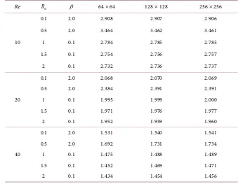
[image:16.595.200.539.465.735.2]chosen as 41 times the radius of cylinder, which is a fairly a large space to acquire accurate results. Table 1 lists the values of drag coefficient for different
Table 1. Grid independence test: Drag coefficients obtained in 64 × 64, 128 × 128 and 256 × 256 grids. The results show that the computation in 128 × 128 grid is optimum.
Re Rm β 64 ×64 128 ×128 256 ×256
10
0.1 2.0 2.908 2.907 2.906 0.5 2.0 3.464 3.462 3.461 1 0.1 2.784 2.785 2.785 1.5 0.1 2.754 2.756 2.757 2 0.1 2.732 2.736 2.737
20
0.1 2.0 2.068 2.070 2.069 0.5 2.0 2.384 2.391 2.391 1 0.1 1.995 1.999 2.000 1.5 0.1 1.971 1.976 1.977 2 0.1 1.952 1.959 1.960
40
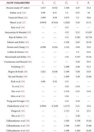
DOI: 10.4236/ajcm.2017.73021 259 American Journal of Computational Mathematics Table 2. Comparison of flow parameters for Re = 40 with available data in literature for zero magnetic field case, that is for β=0. Here, lS is the separation length measured from the center of the circular cylinder.
FLOW PARAMETERS CP CV CD lS θS
Present study (4th order) 1.017 0.532 1.549 5.47 53.4
Sekhar et al.[24] 0.99 0.51 1.5 5.57 54 Tuann & Olson [26] 1.095 0.58 1.675 5.2 54.8
Bharti et al.[27] 0.9976 0.5316 1.5292 5.45 53.71 Kim et al.[36] --- --- 1.51 --- --- Sanyasiraju & Manjula [39] --- --- 1.53 5.21 51.025
Raju & Sekhar [40] --- --- 1.51 5.383 52.734 Takami and Keller [42] --- --- 1.536 5.65 53.55 Dennis and Chang [43] 0.998 0.524 1.522 5.69 53.8
Collins & Dennis [44] --- --- --- 5.3 53.6 Nieuwstadt and Keller [45] --- --- 1.55 5.357 53.34 Coutanceau and Bouard [46] --- --- --- 5.26 53.5
Fornberg [47] --- --- 1.498 5.48 51.5 Rogers & Kwak [48] 1.011 0.538 1.549 5.58 53.0 He and Doolen [49] --- --- 1.499 5.49 52.84
Park et al.[50] 0.99 0.52 1.51 --- --- Ye et al.[51] --- --- 1.52 5.54 --- Niu et al.[52] --- --- 1.574 5.51 53.8 Silva et al.[53] --- --- 1.54 --- --- Tseng and Ferziger [54] --- --- 1.53 5.42 --- Chakraborty et al.[55] 0.9943 0.5229 1.5172 5.21 53.6
Dinget al.[56] --- --- 1.713 5.4 53.5 Shu et al.[57] --- --- --- 5.40 --- Udhayakumar et al.[58] --- --- 1.583 5.338 53.43 Udhayakumar et al.[59] --- --- 1.596 5.387 53.88 Udhayakumar et al.[60] --- --- 1.598 5.382 53.85
Re and for three different grids in presence of magnetic field. From the table, it
is noted that 128 128× grid is found to be optimum. Further refining of grids,
that is employing 512 512× , etc. will not give more accuracy because the
accuracy of the numerical scheme is decided by method of discretization and not
by the fineness of grid. Table 2 shows the comparison of flow parameters
obtained using our numerical scheme with the data available in the literature [24] [26] [27] [36] [39] [40] [42]-[60]. For the zero magnetic field
(
β =0)
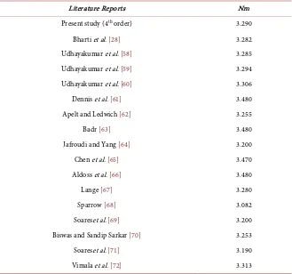
case,DOI: 10.4236/ajcm.2017.73021 260 American Journal of Computational Mathematics Table 3. Comparison of results for Mean Nusselt number (Nm) in the absence of external magnetic field for Re = 40 and Pr = 0.73.
Literature Reports Nm
Present study (4th order) 3.290
Bharti et al.[28] 3.282 Udhayakumar et al.[58] 3.285 Udhayakumar et al.[59] 3.294 Udhayakumar et al.[60] 3.306 Dennis et al.[61] 3.480 Apelt and Ledwich [62] 3.255
Badr [63] 3.480
Jafroudi and Yang [64] 3.200 Chen et al.[65] 3.470 Aldoss et al.[66] 3.480
Lange [67] 3.280
Sparrow [68] 3.082
Soareset al.[69] 3.200 Biswas and Sandip Sarkar [70] 3.253 Soareset al.[71] 3.190 Vimala et al.[72] 3.313
present work which is attributed to the higher order numerical scheme employed in contrast to traditional first or second order accurate data in the
literature. Further the data for mean Nusselt number Nm is also compared
against other reported data [28] [58]-[72] and it is tabulated in Table 3. It is observed that out of the data shown in table, 71% of researchers have reported the value of mean Nusselt number close to our value of 3.29, whereas others have reported a higher value close to 3.48. The only value which departs from the rest is that reported in [68].
5. Results and Discussion
The response of separation length
( )
ls and the separation angle( )
θs of the recirculation bubble with the Alfvén number( )
β is presented in Figure 2. The separation length reduces strongly with small magnetic fields given by β <1. Further increase of β suppresses the separation only to a little extent. The ratio of inertial to Lorentz force is considered as friction parameter given by Re Hais also equal to Re N . The Hartmann layer is damped by the inverse friction
parameter [38] and hence wake suppression is observed. From the plot of
DOI: 10.4236/ajcm.2017.73021 261 American Journal of Computational Mathematics Figure 2. Comparison of the separation length ls and separation angle θs computed
using the present fourth order scheme with second order scheme.
is required for the same level of wake suppression. The Lorentz force will directly change the fluid velocity and according to Equation (2) and hence the vorticity of the fluid changes due to applied magnetic field. Together with a gradual decrease in the length of the standing vortex near the cylinder, a growing region of positive vortices are seen when the magnetic field strength is increased (not shown) and this is also predicted theoretically [73]. The positive contours of ω are not present when N=0. The region of positive vorticity
gets directed towards the center and extends in the upstream with increasing magnetic field or with increasing the conductivity of the fluid. This pushes the negative vorticity region be form at far distance [17]. Since the induced magnetic field is taken into consideration in the formulation of the problem, the magnetic stream function A is computed according to Equation (60) during the solution procedure, which is substituted in Equations ((12) and (13)) to get the effective or total magnetic field components. The contours of the lines are presented in
Figure 3 for Rm =1 with varying β. From this contour plot, we observer that
the magnetic field is no longer uniform in the entire flow region. This is due to the current density which got generated in the fluid by virtue of its motion and, in turn, the applied magnetic field is modified. In regions near θ =90, the
induced magnetic field is added to the applied field, while in the other upstream and in the wake regions, the induced magnetic field has opposed the applied field resulting in a lower magnetic field. Also, as β increases, we observe more changes to the resultant magnetic field.
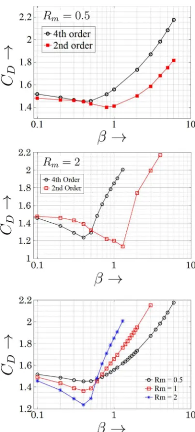
The dependence of pressure drag coefficient CP, viscous drag coefficient CV,
and total drag coefficient CD on β and Rm are shown in Figure 4. The
DOI: 10.4236/ajcm.2017.73021 262 American Journal of Computational Mathematics scheme. The top and middle plots show the comparison of results obtained from the present work with that obtained using a second order accurate scheme.
Table 4 shows a detailed comparison of drag coefficients and flow separation
parameters. For small values of magnetic Reynolds number Rm the total drag
coefficient decreases when β ≈0.5 and then the drag coefficient increases for higher β. This is in contrast to the result obtained using second order method where it is predicted that the drag coefficient minimum takes place when β1, which are noted from the red color data points of top and middle plots. The
increase of drag coefficient following the
(
)
1 2N Re power-law with N is
[image:20.595.212.532.243.701.2]predicted theoretically [17] and the existence of a minimum drag coefficient for certain magnetic field is also reported [74].
DOI: 10.4236/ajcm.2017.73021 263 American Journal of Computational Mathematics Figure 4. Comparison of second order and fourth order accurate calculation of total drag coefficient CD (top and middle). It is noted that for higher values of Rm, the fourth
order results show a larger deviation from the second order results. The bottom one shows the effect of magnetic Reynolds number on CD.
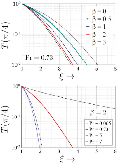
The forced convective heat transfer in the fluid flow is studied for Re=40
with 0≤Rm≤2, 0≤ ≤β 50 for Prandtl numbers 0.065, 0.73, 5, 7 which may
represent typical fluids like liquid metals, air, KOH and water respectively. The surface Nusselt number on the surface of the cylinder and its effect on the magnetic field is shown in Figure 5 (bottom plot). In the absence of external magnetic field Nu decreases on the surface of the cylinder until the separation
DOI: 10.4236/ajcm.2017.73021 264 American Journal of Computational Mathematics Table 4. Drag coefficients and flow separation parameters for Re = 40 and its comparison with second order results.
Rm β CP CP
[24] CV C
V
[24] CD C
D
[24] lS l
S
[24] θS θ
S
[24]
[image:22.595.207.537.101.691.2]0 0 1.017 0.99 0.532 0.51 1.549 1.50 5.47 5.57 53.4 54 0.5 0.4 0.947 0.94 0.505 0.50 1.452 1.40 3.23 4.5 47.8 52.5 0.5 0.8 0.991 0.91 0.522 0.485 1.514 1.405 2.25 3.25 41.5 48 0.5 1 1.023 0.90 0.535 0.48 1.558 1.38 2.04 2.9 39.4 46.5 0.5 4 1.342 1.11 0.642 0.57 1.984 1.68 1.16 1.5 17.6 29 0.5 6 1.489 1.42 0.688 0.60 2.177 2.02 1.00 1.25 4.9 22 1 0.4 0.884 0.93 0.479 0.48 1.363 1.41 2.49 4.1 43.6 51.5 1 0.8 1.033 0.86 0.536 0.46 1.570 1.32 1.57 2.55 31.6 44.5 1 1 1.098 0.87 0.56 0.47 1.658 1.34 1.43 2.12 28.1 40.8 1 3 1.472 1.17 0.681 0.59 2.153 1.76 1.00 1.25 28.1 20.1 2 0.2 0.887 0.95 0.482 0.51 1.369 1.46 3.32 4.95 48.5 52.8 2 0.4 0.794 0.90 0.441 0.43 1.235 1.33 1.86 3.83 37.3 50.9 2 0.8 1.139 0.78 0.568 0.44 1.708 1.22 1.11 1.95 14.8 39.7 2 1 1.244 0.77 0.618 0.43 1.906 1.21 1.05 1.49 8.4 30.5
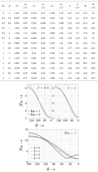
Figure 5. Angular variation of Nusselt number and its influence on magnetic Reynolds number and the strength of magnetic field. Here, Re=40 and Pr=0.73 (top) and
7
DOI: 10.4236/ajcm.2017.73021 265 American Journal of Computational Mathematics which is the rear stagnation point (red, black and blue lines). That is, along with suppression of flow separation, the enhancement of heat transfer is also suppressed. These effects proportionally increase for fluid with higher Prandtl numbers. The application of external magnetic field causes the thickness of the viscous boundary layer to increase. The maximum heat transfer region lies in the front stagnation point. At this point the magnetic field casus a decrease in Nu. The effect of electrical conductivity on the Nu is shown in Figure 5 (top plot). By considering the low magnetic case
(
β =0.5)
, in the upstream region, theheat transfer is higher for a fluid with lower conductivity. However, the reverse in true in the downstream region. This kind of non-monotonic behavior can be nullified, if the same experiment is repeated for a higher magnetic field, say
1
β = . These effects are due to the change in radial and angular velocities of the fluid by the application of external magnetic field. Figure 6 shows the variations
of mean Nusselt number with β. For weak magnetic field strengths, the mean
Nusselt number reduces when compared to the zero magnetic field case. This
happens until a critical field value of β =0.5 [Figure 6 (bottom)]. For
0.65
β = , the mean Nusselt number converges to a single value Nm=2.6,
independent of electrical conductivity of the fluid. The critical field divides the plot into two regions: For β <0.4, the mean Nu increases with conductivity of the fluid. For β >0.65 the higher conductivity of the fluid aids to increase the
heat transfer. Thus the mean Nusselt number Nm depends non-monotonically
[image:23.595.275.473.409.687.2]with the electrical conductivity Rm of the fluid. In the region 0.4≤ ≤β 0.65