The effect of learning on climate policy under fat tailed uncertainty

Munich Personal RePEc Archive

The effect of learning on climate policy

under fat-tailed uncertainty

Hwang, In Chang and Reynes, Frederic and Tol, Richard

13 February 2014

Online at

https://mpra.ub.uni-muenchen.de/53681/

1

The Effect of Learning on Climate Policy under Fat-tailed Uncertainty

In Chang Hwanga,*_{,Frédéric Reynès}a,e,f _{and Richard S.J. Tol}b,a,c d,g

a

Institute for Environmental Studies, Vrije Universiteit, De Boelelaan 1087, 1081 HV,

Amsterdam, The Netherlands

b

Department of Economics, University of Sussex, Jubilee 281, Falmer, Brighton, BN1 9SL,

United Kingdom

c

Department of Spatial Economics, Vrije Universiteit, De Boelelaan 1105, 1081 HV,

Amsterdam, The Netherlands

d

Tinbergen Institute, Gustav Mahlerplein 117, 1082 MS, Amsterdam, The Netherlands

e_{OFCE Sciences Po’s Economic Research Centre,}

rue Saint Guillaume, 75337, Paris,

France

f

TNO - Netherlands Organisation for Applied Scientific Research, Van Mourik

Broekmanweg 6, 2600 AA, Delft, The Netherlands

g

CESifo, Munich, Germany

* Corresponding author. VU University Amsterdam, Institute for Environmental Studies, De

Boelelaan 1087, Amsterdam, The Netherlands, 1081 HV (Tel.: +31 6 1602 5459, Fax: + 31

(0) 20 59 89553, E-mail address: [email protected])

Abstract

We construct an endogenous (Bayesian) learning model with fat-tailed uncertainty on the

equilibrium climate sensitivity and solve the model with stochastic dynamic programming. In

our model a decision maker updates her belief on the climate sensitivity through temperature

observations each time period and takes a course of action (carbon reductions) based on her

belief. We find that the uncertainty is partially resolved over time, although the rate of

2

efforts to reduce carbon emissions relative to the no-learning case. The larger the tail effect,

the larger the counteracting learning effect. Learning at least partly offsets the tail-effect of

deep uncertainty. This is intuitive in that the decision maker fully utilizes the information

revealed to reduce uncertainty, and thus she can make a decision contingent on the updated

information. In addition, with various scenarios, we find that learning enables the economic

agent to have less regrets for her past actions after the true value of the uncertain variable

turns out to be different from the initial best guess. Furthermore the optimal decisions in the

learning case are less sensitive to the true value of the uncertain variable than the decisions in

the uncertainty case. The reason is that learning lets uncertainty converge to the true value of

the state in the sense that the variance approaches 0 as information accumulates.

Key words

Climate policy; deep uncertainty; Bayesian learning; integrated assessment; stochastic

dynamic programming

JEL Classification

Q54; C61; Q58; H23

1 Introduction

“The acquisition of information has value, which it would not have in a world of certainty.”

(Arrow, 1957: 524) Following this notion, economists have investigated the effects of

learning on policy and welfare, including the irreversibility effect, the value of information,

the optimal timing of action, the rate of learning, the direction of learning, and the cost of

learning.1 The answers to these questions, however, are not straightforward especially when

1

Some earlier papers, not exhaustive, for these issues on climate change are the followings: the irreversibility

3

climate policy is concerned. They depend not only on the ways that climate feedbacks,

preferences, and economic impacts are considered, but also on the ways that uncertainty and

learning are introduced.

The general framework for the problem of decision making under uncertainty and learning

about climate change is as follows (Pindyck, 2002). In an economy where the impacts of

climate change are uncertain with a possibility of learning, a decision maker encounters

conflicting risks: a risk that stringent emissions control today turns out to be unnecessary ex

post, and a risk that much stronger efforts are required in the future since climate change is

catastrophic. If there is no irreversibility to be considered, the problem becomes trivial since

the decision maker can revise her actions as and when required. However, both the

investment in emissions abatement and the accumulation of greenhouse gases (GHGs) are, at

least partially, irreversible.

In the presence of irreversibility, the decision maker generally favors an option that

preserves flexibility (Arrow and Fisher, 1974; Henry, 1974). As far as climate policy is

concerned, however, since there are two kinds of counteracting irreversibility, the problem

becomes complicated. The relative magnitude of irreversibility determines the direction and

the magnitude of the effect of learning on climate policy: the irreversibility related to the

carbon accumulation strengthens abatement efforts, whereas the irreversibility related to the

capital investment on emissions abatement lowers abatement efforts.

Popp, 1997); the optimal timing of action (Pindyck, 2002; Guillerminet and Tol, 2008); the rate of learning

(Kolstad, 1996b; Kelly and Kolstad, 1999; Leach, 2007; Webster et al., 2008); and the direction of learning

4

Alternatively, we can think of the problem as experimentation with carbon emissions in the

framework of learning by doing (Arrow, 1962).2 The decision maker confronted with

uncertainty and a possibility of learning about climate change can be seen as a Bayesian

statistician who experiments with a level of carbon emissions to gain information about

uncertainty. The more GHG emissions (in turn, the higher warming) are more informative in

the sense that it provides more precise information about uncertain parameters such as the

equilibrium climate sensitivity.3 However, the acquisition of information comes at an

(implicit) cost: higher emissions induce consumption losses (via increased temperature). As a

result, the decision maker should choose an optimal level of emissions by comparing gains

and losses from the acquisition of information.

In the literature, the possibility of learning generally affects the near-term policy towards

higher emissions relative to the case where uncertainty is not reduced (for the summary of the

literature see Ingham et al., 2007). One of the reasons is that irreversibility constraints such as

the non-negativity of carbon emissions rarely bite in climate change models (Ulph and Ulph,

1997).4 In addition, even if they do bind, the effect of the irreversible accumulation of the

2

Learning in the current paper is ‘passive’ in a sense that the decision maker does not directly affect the rate of

learning. Usually in the ‘active’ learning literature (also known as dual control, probing, or optimal experimentation), control variables play a direct role in reducing uncertainty (e.g. Prescott, 1972; Grossman et

al., 1977). See Kendrick (2005) for more on this issue.

3

The equilibrium climate sensitivity is a measure of the responsiveness of the climate system to radiative

forcing. It denotes how much atmospheric temperature changes when carbon dioxide concentration is doubled.

4

Regarding this, Webster (2002) argues that if the non-negativity matters, the effect of the irreversible

5

carbon stocks is smaller than the effect of irreversible capital investment on emissions

abatement (Kolstad, 1996a; 1996b).5

If we think of the results in the framework of learning by doing, these results imply that

more carbon emissions are more informative in the sense that the decision maker can attain

more utility from her experimentation (Blackwell and Neyman, 1951).

Fat-tailed (or deep, structural) uncertainty may lead to different results since the marginal

damage costs of climate change become far larger, if not arbitrarily large, under deep

uncertainty (Weitzman, 2009).6 Consequently, this may change climate policy in favor of

stringent efforts to reduce GHG emissions compared to the no learning case. However,

learning may of course reveal thin-tailed uncertainty about objective function, weakening the

case for emissions control.7 Put differently, learning may reduce the optimal level of

emissions control even when we account for deep uncertainty.

A dynamic model on climate change incorporating deep uncertainty and learning is

developed in this paper.8 Learning in the model is endogenous: the decision maker updates

5

There are some papers that find the case where the irreversibility constraints (i.e. nonnegative emissions) bind

with various methods, including the alternative parameterization of some critical equations (Ulph and Ulph,

1997; Webster, 2002), the introduction of catastrophic events (Keller et al., 2004), and the presence of stringent

climate targets (Webster et al., 2008).

6

This paper retains the following definition of fat tail: “a PDF [probability density function] has a fat tail when its moment generating function is infinite ‐ that is, the tail probability approaches 0 more slowly than

exponentially” (Weitzman, 2009: 2).

7

Notice that the posterior distribution of the climate sensitivity always has fat tails in the learning model of this

paper (see Section 2). However, social welfare may have thin tails as the variance parameter of the climate

sensitivity approaches zero over time.

8

6

her belief about an uncertain parameter, expressed in a probability distribution, by the

acquisition of information. This approach on endogenous learning is not new in the

economics of climate change. For instance, Kelly and Kolstad (1999) introduce uncertainty

about a climate parameter (linearly related to the climate sensitivity) into the DICE model

(Nordhaus, 1994), and then investigate the expected learning time. Leach (2007) follows a

similar model and approach, but introduces an additional uncertainty on climate parameters.

Webster et al. (2008) investigate the effect of learning on the near term policy using the

DICE model with a discrete four-valued climate sensitivity distribution and exogenous

learning. In the second part of their paper, they investigate the time needed to reduce

uncertainty about the climate sensitivity and the rate of heat uptake by using a simplified

climate model. They incorporate fat-tailed uncertainty and Bayesian learning into the model

but their model does not analyze policy.

In the current paper another perspective is added compared to the literature. That is, where

previous papers mostly studied thin-tailed distributions, we here focus on fat-tailed ones.

Kelly and Tan (2013), although not published yet, do a similar analysis as ours.9 They

incorporate fat-tailed uncertainty into a model of climate and the economy and consider the

effect of learning on policy. They find that with learning the decision maker can reject the

maker in our model can and do postulate probability distributions of uncertain variables, ex ante. Although the

distinction between risk and uncertainty is important, we here use the terms interchangeably as the other climate

change literature usually do. The decision making under ambiguity requires a different framework (e.g. Gilboa

and Schmeidler, 1989) and thus it is beyond the scope of the current paper. See Millner et al. (2013) for an

application of ambiguity theory into an integrated assessment model (IAM).

9

The difference between ours and Kelly and Tan (2013) was more transparent at the time when the first draft of

the current paper was made available (Sussex Working Paper No. 53-2012 with the same title). The previous

7

fat-tailed portion of the distribution in a decade or so, and that the optimal carbon tax in the

learning model decreases by about 40-50% compared to the no-learning case.

There are some differences between Kelly and Tan (2013) and our analysis. First, the

model, calibrations, the definition of learning, and solution methods are different. For

instance, Kelly and Tan apply the model of Bartz and Kelly (2008), the damage function of

Weitzman (2009), a well-mixed single-layered climate model, the definition of learning by

Kelly and Kolstad (1999), and spline approximations, whereas we use the original DICE

model (Nordhaus, 2008), the damage function of Nordhaus (2008), multi-layer climate

system, the definition of learning by Webster et al. (2008), and logarithmic approximations.

These differences may induce a different rate of learning and correspondingly find a different

magnitude of the learning effect.10

Second, the main focus is different between the two papers. The current paper explicitly

deals with the benefits of learning in terms of the expected social costs of climate change,

whereas Kelly and Tan focus on the rate of learning and the effect of diminishing fat tails.

The other benefits of learning are also discussed in the current paper.

Third, on the results side, the optimal policy converges to the case of perfect information in

about two decades in Kelly and Tan (2013); our model converges more slowly. The main

reason is that the rate of learning (measured as the reduction of variance) is much faster in

their model than in ours.11 Their rate of learning is also far faster than the earlier literature

10

For instance, the multi-layered climate model may alter the rate of learning compared to the single-layered

model. This is because the other layers such as the deep ocean serve as a heat reservoir.

11

Their results are largely dependent on the (presumably misused) parameterizations for their climate model.

The time is annual in their full model, but the parameter values they used for temperature evolution is the one

8

including Kelly and Kolstad (1999), Leach (2007), and Webster et al. (2008). In addition,

such fast learning is not consistent with the past experiences in climate science (Allen et al.,

2006). Since there is only one policy lever (i.e. GHG emissions) to increase the rate of

learning in such a passive learning model (see footnote 2), the rate of learning is not generally

faster in a model of fat-tailed uncertainty than in a model of thin-tailed uncertainty (see

Section 6). Note that 1) carbon emissions are less under fat-tailed uncertainty than under

thin-tailed uncertainty, and that 2) more warming leads to more precise information.

This paper proceeds as follows. Section 2 describes the model and computational methods.

The DICE model (Nordhaus, 2008) is revised to represent (deep) uncertainty and endogenous

learning about the equilibrium climate sensitivity through the framework of feedback analysis

(Hansen et al, 1984; Roe and Baker, 2007). The model is solved with the method of dynamic

programming. Section 3 presents the posterior distribution of the climate sensitivity and

compares the rates of learning. Section 4 illustrates the effect of learning on climate policy.

The case where the initial belief on the climate sensitivity is unbiased in the sense that the

true value of the climate sensitivity turns out to be the same as the expected value of the

initial belief of the decision maker is investigated. Then the results are compared with the

other cases where the initial belief turns out to be biased. Section 5 investigates the cost of

no-learning. Section 6 presents a sensitivity analysis with the damage function of Weitzman

(2012). Section 7 concludes.

values of the DICE model, of which time is decadal. See Marten (2011) and Cai et al. (2012a) for calibrations

for the climate parameters of DICE with different time horizon. Figure 6 and Table 1 in Kelly and Tan (2013)

imply that learning in their model is far faster than the one in this paper (see Section 3 of this paper for a

literature review on the rate of learning). Applying the same parameterizations (i.e., =0.22 and =0.05) with

Kelly and Tan (2013) to our model, however, fast learning as in Figure 6 of their paper can be obtained (results

9

2 The Model and Methods

2.1 The Revised DICE Model

Uncertainty and learning are introduced in the DICE model (more precisely, the DICE

2007 optimal policy version). There are several differences in the model of this paper with

the original DICE model. First, the current model incorporates (deep) uncertainty. The key

uncertain parameter in the model is the equilibrium climate sensitivity. Second, the

probability density function (PDF) of the climate sensitivity changes over time through

temperature observations. As a result, the parameters of the climate-sensitivity distribution

become endogenous state variables. Third, stochastic temperature shocks are introduced for

Bayesian updating on the distribution parameters.12 Fourth, time horizon and a solution

method are different. More precisely, the time period in our model is annual and thus some

parameter values are adjusted. A solution method suitable for an (infinite horizon)

endogenous learning model is applied in this paper. There is no upper bound of accumulated

carbon emissions in the current model and backstop technology is not considered in the paper.

Finally, the savings’ rate is fixed at constant in our model for simplicity. These assumptions

do not affect the main results of the current paper qualitatively.13 Learning is costless in the

12 _{Temperature shocks reflect observational errors, model’s biases to match observations, and the natural}

variability (Webster et al., 2008).

13

The savings rate (defined as the gross investment divided by the net production) changes in the range of

0.240 and 0.247 for the first 600 years in the DICE-CJL model (Cai et al., 2012a), which is a modified version

of DICE with an annual time step. Fixing the savings’ rate at a reasonable value does not have much impact on the results of the model. For instance, if the savings’ rate is fixed at 0.245 all variables including the optimal carbon tax deviate only less than 3% from the original results. This holds even if the true value of the climate

10

model, for simplicity. Unless otherwise noted, the parameter values and the initial values for

the state variables (in the year 2005) are the same as in DICE 2007.

The decision maker of the model chooses the rate of emissions control in each time period

so as to maximize social welfare defined as in Equation (1) – the expected discounted sum of

utility of per capita consumption. A unit increase in GHG emissions induces future climate

change and thus it reduces expected utility, due to the loss of future consumption as a

consequence of higher warming. Emissions control comes at a cost and the cost is increasing

and convex in the emissions control rate. Gross output net of damage costs and abatement

costs is allocated into investment and consumption.

∑

∑ ⁄

(1)

subject to

[

] (2)

(3)

where is the expectation operator given information at point in time t, is the

instantaneous utility function of per capita consumption, is consumption, is labor force

(exogenous), is the total factor productivity (exogenous), (= ) is the abatement

costs function, (=1/( )) is the damage function, (= ) is the

production function, is the emissions control rate, (= ) is gross investment, (=0.245)

11

consumption, is the discount factor, (=0.015) is the pure rate of time

preference, (=0.3) is the elasticity of output with respect to capital, (=0.1) is the

depreciation rate of the capital stock, and (=0), (=0.0028388), (=2), (=0.0561), and

(=2.887) are parameters.

The carbon-cycle model is composed of three layers for GHG: the atmosphere, the upper

ocean, and the lower ocean. The rate of GHG mixing between layers is captured by ,

where iand j denote each layer.

(4)

(5)

(6)

where , , are the carbon stocks in the atmosphere, the upper ocean, the lower

ocean, respectively, is the emission-output ratio (exogenous), is GHG emissions

from non-energy sectors (exogenous), and (=0.9810712), (=0.0189288), (=0.0097213),

(=0.005), (=0.0003119), and (=0.9996881) are climate parameters adjusted for annual time

step following Cai et al. (2012a).

In a general integrated assessment model (IAM) the temperature response is usually

modeled as having one or two boxes, and those can be derived from the energy balance

model of Baker and Roe (2009). The mixed layer exchanges heat with the atmosphere and the

12

simplification (the mixed layer and the deep ocean) and a discrete time horizon, the energy

balance model becomes the temperature response model of DICE (Marten, 2011):

{

} (7)

{ } (8)

where is radiative forcing from non-CO2 gases (exogenous), (=596.4GtC) is the

pre-industrial carbon stock in the atmosphere, is the equilibrium climate sensitivity, (=0.022),

(=0.3), (=0.005), and (=3.8) are climate parameters adjusted for annual time step following

Cai et al. (2012a), and , where =1.2°C/2xCO2 is the reference climate sensitivity

(absent of climate feedbacks: black-body planet).

2.2 Bayesian Learning

The climate sensitivity has a highly skewed distribution to the upper end (see Figure 1) in the

model with parameters ̅ and _√ as follows.

(

√ )

{ [

( ̅ ₎ ]

}

(9)

The above equation is derived in the framework of feedback analysis (Roe and Baker,

2007) using the fact that the climate sensitivity is related to the total feedback factors as in

13

⁄ (10)

where is the total feedback factors which measures aggregate impacts of physical factors

such as water vapor and cloud on radiative forcing in a way to magnifying the response of the

climate system (Hansen et al., 1984). is assumed to be normally distributed with mean ̅

and variance and the initial value for ̅ and are 0.65 and 0.132, respectively,

following Roe and Baker (2007).

Substituting Equation (10) into Equation (7) and adding stochastic temperature shocks lead:

(11)

where is stochastic temperature shocks and , , ,

, and are adjusted parameters.

The temperature shocks are assumed to have a normal distribution with mean 0 and a

constant variance (=0.12) following Tol and de Vos (1998). Although the shocks are

independent, Equation (11) implies a first-order autoregressive model (see Kelly and Kolstad,

1999). In this representation, the decision maker expects that air temperature in the next

period is determined by the following equation: .

However, the actual realization of the temperature is determined not just by the above

equation, but also by the true value of the total feedback factors (which is not known to the

decision maker ex ante with certainty: parametric uncertainty) and by the random realization

14

stochasticity). Put differently, there are deviations between the decision maker’s expectation

and her observations, which lead to the modification of the prior belief.

The decision maker in the model obtains the posterior distribution of the total feedback

factors by the Bayes Rule as follows.

| | (12)

where is the prior belief on the total feedback factors, | is the likelihood

function of the observations given , and | is the posterior belief.

An expert prior for the initial distribution of the total feedback factors is applied in this

paper. More specifically, the normal distribution of Roe and Baker (2007) is used. The

normal prior has some advantages over the other priors such a uniform prior. First, the

posterior calculated from the normal prior is also normally distributed, provided that the

likelihood function is normal. In this case, it is easy to calculate the posterior just by

investigating the posterior mean and the variance (Cyert and DeGroot, 1974). Second, as

Annan and Hargreaves (2011) point out, uniform priors usually used in a Bayesian analysis

assign too much probability to extreme parameter values (say, the climate sensitivity of

10°C/2xCO2) beyond the current scientific knowledge. This assignment may dominate the

calculation of expected damage costs.

The resulting posterior has the normal distribution with mean ̅̅̅̅̅ and variance as in

Equation (13) and (14). These equations are derived from a direct application of the Bayes

Rule with the above mentioned assumptions on the likelihood function and the prior. Note

15

numerically unsolvable since equilibrium cannot be reached (Baker and Roe, 2009). In order

to deal with this issue this paper uses the (unbounded) normal distribution as a prior for

Bayesian updating and then sets an upper bound on the derived posterior distribution for

simulations ( ≤0.999). Note that this upper bound corresponds to the climate sensitivity of

1,200°C/2xCO2. Higher upper bounds than this do not affect the main points of this paper

(results not shown). In the subsequent period, the decision maker uses the previously

calculated posterior as the prior (unbounded normal distribution) for next updating. In this

way, the decision maker updates her belief every time-period.

̅̅̅̅̅ ̅ ⁄ ⁄

(13)

⁄ (14)

Equations (13-14) say that the variance of the total feedback factors decreases over time.

Put differently, the acquisition of information in the model always increases the precision of

the decision maker’s belief. As the variance gets smaller, the mean of the total feedback

factorsapproaches to the (pre-specified) true value, on average. That is, there is no ‘negative’

learning (Oppenheimer et al., 2008) in this model. Although the variance parameter becomes

smaller as temperature observations accumulate, however, the climate sensitivity has still a

16

2.3 Computational Methods

Two kinds of methods have been used for solving a learning model numerically in the

literature: stochastic optimization and dynamic programming. The first one is to consider

possible states of the world on parameter values of interest with corresponding probability

distributions, and solve for the optimal time path of policy variables that maximize the

expected value of the objective function over a finite time horizon (e.g. Kolstad, 1996a;

Webster et al., 2008). The second one is to formulate the problem recursively through a

functional equation and then solve the problem over an infinite time horizon (e.g. Kelly and

Kolstad, 1999; Leach, 2007). The current paper takes the second approach: dynamic

programming.14

General approach of this paper is illustrated below. The solution methods in detail

including accuracy tests are given in Appendix A. Equation (1) is reformulated using the

Bellman equation:

(15)

where is the value function starting from period t, is the vector of control

variables ( ), is the vector of state variables ( , , , , , ̅, v, L, A, ), and

is the vector of uncertain variables (f, ).

Then the value function is approximated with a flexible basis function having a specific

analytic form such as polynomials or logarithmic function. Following this way, the

14

See Bellman and Dreyfus (1962), Stokey and Lucas (1989), Rust (1996), Judd (1998), and Miranda and

17

maximization problem is changed into the regression problem of finding that minimizes

the approximation errors.

∑ (16)

where is the basis function, is the vector of coefficients for the basis function.

The algorithm for finding is summarized as follows. First, choose an initial guess .

Second, simulate a time series satisfying the first order conditions for Equation (15) (see

Appendix A), the initial conditions for the state variables, and the transitional equations (3-8)

and (13-14). Note that if is chosen, the control variables are calculated from the first

order conditions, the initial conditions for the state variables, and the transitional equations.

In this way, the resulting time series depend on the initial guess . Third, calculate the left

hand side (LHS) and the right hand side (RHS) of Equation (15) using Equation (16), the

utility function, and the simulated time series of variables. For the calculation of the

expectation, the Gauss-Hermite quadrature method is applied in this paper (Judd, 1998).

Fourth, compare the calculated values for LHS and RHS of Equation (15) and stop the

iteration if the approximation errors are smaller than the pre-specified tolerance level (the

stopping rule: see Appendix A). Fifth, if the fourth step does not meet the stopping rule,

estimate ̂ that minimizes the approximation errors. Update following the pre-specified

updating rule (see Appendix A). This is a new guess . Then go back to the second step

with the new guess and follow the next steps until the iteration meets the stopping rule.

The algorithm, which is proposed by Maliar and Maliar (2005), effectively reduces the

18

conditions (Judd et al., 2011). By the fixed point theorem, the solution is the unique

solution for the optimization problem (Stokey and Lucas, 1989).

Most literature solving an integrated assessment model of the economy and climate change

with dynamic programming take a similar approach to the methods above. The problem is

formulated in a recursive way and the value function is approximated to a flexible basis

function.15 The fixed-point theorem is applied to search for solutions. The main difference

between papers is the approximation method applied. For instance, Kelly and Kolstad (1999)

and Leach (2007) use neural networks, Kelly and Tan (2013) apply spline approximation, and

Cai et al. (2012b) and Lemoine and Traeger (2014) apply Chebyshev polynomials. Another

difference is the method for dealing with time dependence. For instance, Kelly and Kolstad

(1999), Leach (2007), and Lemoine and Traeger (2014) add the time variable as an argument

for the value function. Cai et al. (2012b) let the coefficient of the basis function vary each

time period. Kelly and Tan (2013) make the model time independent. This paper adds the

time dependent exogenous variables as arguments for the value function. In addition, the

solution method of this paper differs from the literature in that it searches for solutions on an

ergodic set, whereas the other papers generally search for solutions on a carefully designed

grid.

15

Hennlock (2009) also approximates the value function to an analytical basis function, although he solves his

19

3 Learning about the Climate Sensitivity Distribution

The climate sensitivity distribution is the decision maker’s belief on the climate sensitivity

and ̅ and are the parameters of the climate sensitivity distribution.16 According to the

updating procedure presented in the previous section and Appendix A, the belief of the

decision maker on the parameter values of the climate sensitivity distribution changes as

temperature observations accumulate.

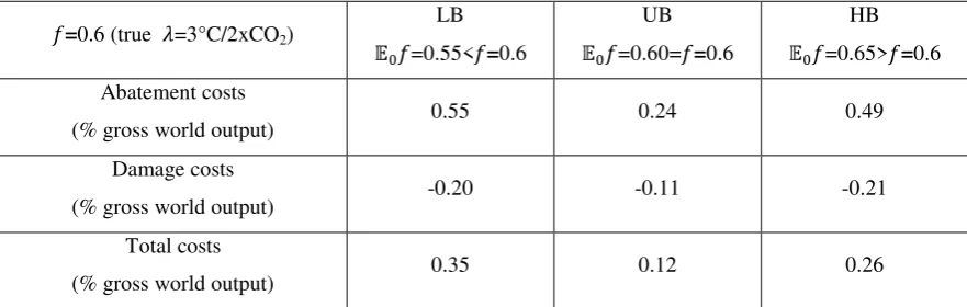
Figure 1 shows the evolution of the belief over time. For Figure 1 and subsequent figures,

=0.65, =0.13 following Roe and Baker (2007) and the true value of is 0.6, of which

corresponds to =3°C/2xCO2. 17

The main implications of this paper do not change

qualitatively for the other values of (results not shown). Considering random realizations

of temperature shocks, we present the average of 1,000 Monte Carlo simulations throughout

the paper for the learning case.

As argued in the previous section, the mean approaches the true value of the total feedback

factors and the variance decreases as the temperature observations accumulate over time (see

the left panel). Since the mean of the climate sensitivitychanges, the coefficient of variation

of the climate sensitivity, the (simulated) variance divided by the (simulated) mean, is

16

Note that is the standard deviation not of the climate sensitivity, but of the total feedback factors. The

standard deviation of the climate sensitivity does not exist, by definition, since it has fat tails.

17

̅ and are the parameters of the climate sensitivity distribution. Note that is the standard deviation not

of the climate sensitivity, but of the total feedback factors. The standard deviation of the climate sensitivity does

not exist, by definition, since it has fat tails. The climate sensitivity distribution is the decision maker’s belief on the climate sensitivity. Our model assumes that the current knowledge of the decision maker on the climate

sensitivity is represented by the distribution with the parameters ̅=0.65 (or 0.60 or 0.55 according to scenarios)

and =0.13. The main implications of this paper do not change qualitatively with the other values of . An

20

considered as a measure of uncertainty in this paper. Learning is defined in this paper as a

decrease in the coefficient of variation similar to Webster et al. (2008). In this definition, the

decision maker learns every time period as seen from the top panels. However learning is

relatively slow. For instance, it takes 55 (230) years for the coefficient of variation to be

reduced to a half (a tenth) level. Time needed to reduce uncertainty is, of course, sensitive to

the specification of the model, especially to the assumptions on the prior and the likelihood

function. However, notice that the results presented in this paper are based on the current

scientific knowledge about the climate sensitivity distribution following Roe and Baker

(2007).

The bottom panels show the corresponding climate sensitivity distributions. The density on

the tails becomes much smaller as time goes by, and thus the precision (defined as the

reciprocal of variance) of the belief increases.

Webster et al. (2008) define learning similar to this paper and the learning time for 50%

reduction in the coefficient of variation of the climate sensitivity is about 60~70 years (when

the distribution of Forest et al. (2002) is used as a prior, see Figure 10 of their paper), which

is largely consistent with the results of this paper. Kelly and Kolstad (1999), Leach (2007),

and Kelly and Tan (2013) define learning as the estimated mean approaching its true value.

That is, learning takes place in their models when the mean of the uncertain variable becomes

statistically close to the pre-specified true value (e.g., the significance level of 0.05).

According to their criterion, the expected learning times are about 146 years (when the true

climate sensitivity is 2.8°C/2xCO2) in Kelly and Kolstad (1999) and the order of hundreds (or

thousands) of years in Leach (2007). The difference between the two papers originates from

21

about 64 years (when the true climate sensitivity is 2.76°C/2xCO2) in Kelly and Tan (2013),

which is far faster than the one in Kelly and Kolstad (1999) and Leach (2007).

Since the definition of learning is different, it is not easy to compare the results of Kelly

and Kolstad (1999), Leach (2007), Kelly and Tan (2013), and the result of this paper directly.

However, we can get some insights from Figures 4, 6 and Table 5 of Kelly and Tan (2013),

Figure 2 of Kelly and Kolstad (1999), and Figure 1 and Table 1 of this paper. If the reduction

of standard deviation is applied as a measure of learning for comparison, Figures 4, 6, 18 and

Table 5 of Kelly and Tan (2013) show that learning is far faster in their model than the model

of this paper. As noted in Section 1 this is primarily because their parameterizations on the

climate parameters are far different from those of this paper and the literature (by a factor of

10).18 Figure 2 of Kelly and Kolstad (1999) implies that there is no much difference in the

learning time between Kelly and Kolstad (1999) and the current paper.

Table 1 illustrates the (upper) tail probability of the climate sensitivity distributions. As

expected, the tail probability decreases as learning takes place. One of the important

questions in climate science is whether or not we can put constraints (or an upper bound) on

the climate sensitivity (Knutti et al., 2002). If we use a specific percentile to impose an upper

bound on the climate sensitivity, the table below gives useful information. For instance, based

on 95th percentile, it takes about 50 years to set an upper bound on climate sensitivity at

6°C/2xCO2.

18

There are also many differences in the model and parameterizations between Kelly and Tan (2013) and the

current paper. For instance, whereas Kelly and Tan (2013) apply the abatement cost function of Bartz and Kelly

(2008), the damage function of Weitzman (2009), a one-box temperature response model, higher consumption

and utility discounting (e.g., the pure rate of time preference is 0.05), this paper applies the abatement cost

function of Nordhaus (2008), without considering backstop technology, the damage function of DICE and

Weitzman (2012), the two-box temperature response model, and lower consumption and utility discounting than

22

The rate of learning is as important as the magnitude of learning since slow learning may

lead to our incapability to take appropriate actions on time because of the possibility of

irreversible changes. Especially when we consider the possibility of (discontinuous) climate

catastrophes such as a collapse of the West-Antarctic Ice Sheet (Guillerminet and Tol, 2008)

and the thermohaline circulation collapse (Keller et al., 2004), we should put more

importance on the rate of learning. See also Lemoine and Traeger (2014) for the effects of

tipping points on climate policy. Furthermore, fast learning enables more efficient allocation

of resources.

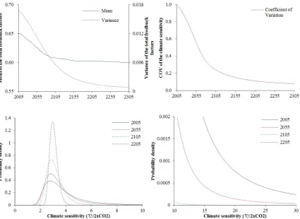
Some sensitivity analyses are presented in Figure 2. Since does not change according

to the cases, the variance parameter of the total feedback factors are compared. The higher

(respectively, lower) is the true value of the climate sensitivity, the faster (resp., slower) is the

learning. This is intuitive in that the higher climate sensitivity implies the higher temperature

increases, resulting in the lower variance parameter (see Equation 14). In a similar fashion,

the rate of learning increases in emissions (results not shown) as shown in Leach (2007).19 A

unit increase (respectively, decrease) in emissions from the optimal path reduces (resp.,

increases) the uncertainty. The more deviations in emissions are the higher deviations in the

rate of learning are. The right panel illustrates the sensitivity of the rate of learning on the

initial level of uncertainty. The variance parameter converges to a low level during the late

22nd century. In other words, differences in the initial level of uncertainty become irrelevant

after 150 years or so. This implies that the rate of learning is higher in a more uncertain case.

Nevertheless, there are substantial differences in uncertainty in the near future.

19

The model is simulated with an additional unit of exogenous carbon emissions. For this simulation, the

solution b of the reference case ( =0.6, =0.60, =0.13) is used as the initial guess. The other specifications

23

The rate of learning is decreasing in the standard deviation of temperature shocks. This is

because as the noise increases observations become less informative (see the bottom left

panel and Equation (14)).

Compared to the reference case where the damage function of Nordhaus (2008) is applied,

the rate of learning is lower if the damage function of Weitzman (2012), Equation (19) in

Section 6, is applied (see the bottom right panel). This is because a unit increase in GHG

emissions is expected to be less beneficial than the reference case in terms of social welfare.

The expected net gains (the difference between the expected gains from reducing uncertainty

and the expected loses from temperature increases) are lower for the highly reactive damage

function than for the less reactive damage function.

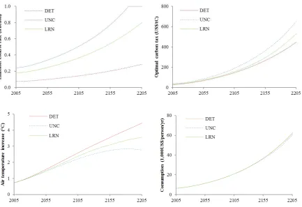
4 The Effect of Learning on Climate Policy

The effect of learning on climate policy is investigated in this section. To this end, the

following three cases are compared: (1) Deterministic, (2) Uncertainty (no learning), and (3)

Learning. The deterministic case refers to the case where the decision maker does not

consider uncertainty or the case where there is no uncertainty. The uncertainty case refers to

the case in which the decision maker accounts for uncertainty, but her belief remains

unchanged. Information may accumulate, but the decision maker simply ignores the

possibility of learning or chooses to ignore information gathered. Finally, the belief of the

decision maker is subject to change in the learning case. The decision maker fully utilizes

information acquired from temperature observations so that she can make a decision

24

Figure 3 summarizes the effect of learning, which is generally consistent with the literature

as we briefly introduced in Section 1. See Table 2 for some numerical values in 2015. First,

the fat-tailed uncertainty increases the abatement efforts relative to the deterministic case.

This is because the uncertainty model considers the less probable but more dismal future as

well as the most probable (mode) or the expected state of the world. Second, the possibility of

learning reduces the abatement efforts relative to the uncertainty case. Although the

atmospheric temperature increases more in the learning case than in the uncertainty case (see

the bottom left panel, this is because carbon emissions are greater in the learning case as a

result of the lower emissions control rate), the decision maker attains (slightly) more

consumption (in turn, utility) from the learning case. This implies that the experimentation

with more emissions (or learning) is beneficial to the decision maker.

5 The Benefits of Learning

5.1 The Optimal Carbon Tax and Social Welfare

In the learning model, atmospheric temperature evolves according to the true value of the

climate sensitivity, but the decision maker conducts a course of action according to her belief.

Then what if the initial belief on the climate sensitivity turns out to be ‘biased’ (in the sense

that the expected value does not equal the true value)? In order to answer the question the

model is simulated with an assumption that the decision maker has a different belief on the

parameter values of the climate sensitivity distribution according to scenarios. The true value

of the climate sensitivity and the initial variance parameter are assumed to be the same across

all scenarios (i.e., true =3°C/2xCO2 and =0.13), but the mean parameter is different between

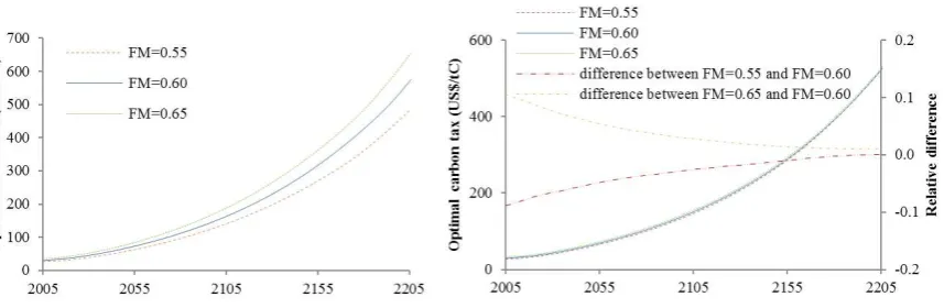
25

Put differently, UB, LB, and HB scenarios stand for unbiased belief, low-biased belief, and

high-biased belief cases, respectively in this section.20

Figure 4 illustrates the results for each scenario. The optimal carbon tax changes a lot

according to the belief of the decision maker in the uncertainty case (see the left panel). The

general trend is that, as expected, the higher is the decision maker’s belief on the climate

sensitivity, the higher is the carbon tax. Compared to the uncertainty case, the differences

among scenarios in the learning case are fairly small and the tax levels converge over time

(see the right panel). This is because learning enables the decision maker to adjust her actions

according to information revealed. The optimal carbon tax is biggest for the HB scenario

( =0.65> =0.6) and lowest for the LB scenario ( =0.55< =0.6) (see also Table 2). However,

as temperature observations accumulate over time the belief of the decision maker

approaches the true value, which is the same across all the scenarios, and thus the difference

in the optimal carbon tax between the scenarios become small in the long run. The rate of

emissions control, temperature increases, and consumption show a similar pattern (results not

shown).

Table 2 illustrates the optimal carbon tax and the net present value of the expected utility

of consumption for each scenario in Figure 4. The optimal carbon tax is higher (lower,

respectively) in the uncertainty case than in the deterministic case, and it decreases (increases,

resp.) in the learning case for the HB and UB scenarios (the LB scenario, resp.). These results

are intuitive in that if the decision maker believes that the climate sensitivity is lower (higher,

20

The model was also simulated with an assumption that the decision maker has the same belief on the

parameter values of the climate sensitivity distribution ( =0.65, =0.13), but the true value is different

between scenarios (e.g., =0.6, 0.65, or 0.7). The general implications of these simulations are similar to the

26

respectively) than the true value, ex ante, her actions become less stringent in the UNC-LB

case compared to the LRN-LB case (the LRN-HB case compared to the UNC-HB case, resp.).

In the UB case, the carbon tax is lower in the learning case because the uncertainty reduces

over time. Numerically learning reduces the effect of deep uncertainty by about 42%.21 In

addition, as shown in Table 2, the uncertainty case is always inferior to the learning case in

terms of utility. Put differently, learning is always valuable in that it increases social welfare.

This is because it allows for a better estimation of the total costs of climate change.

5.2 The Costs of No-learning

In order to see the value of learning in a different perspective, let us suppose that the decision

maker chooses to change her strategy about learning in a specific time period, say in the year

2105. That is, the decision maker starts to update her belief based on temperature

observations after 2105. Under this assumption, the difference in the total costs (the sum of

the damage costs and the abatement costs) between the uncertainty case and the learning case

represents the benefits of learning or penalties for no-learning.

Figure 5 shows the results for the HB scenario ( ). Considering the

differences in gross production and investment between the cases, costs as a fraction of gross

production are presented. As illustrated in the previous section, the optimal rate of emissions

control is lower for the learning case than for the uncertainty case, and thus the abatement

costs are lower but the damage costs are higher for the learning case. The difference in the

abatement costs between the uncertainty case and the learning case decreases after the late

21

This number is calculated as follows. The learning-effect = (the carbon tax for the uncertainty model - the

carbon tax for the learning model) / (the carbon tax for the uncertainty model - the carbon tax for the

27

22th century because the non-negativity constraint of GHG emissions starts to bind for the

uncertainty case. The total costs are lower for the learning case than for the uncertainty case.

For instance, the total costs are 0.26% point (as a fraction of gross world output) lower for the

learning case than for the uncertainty case in 2105.

Table 3 illustrates the results for the year 2105. The cost of no learning in 2105 reduces to

0.12% point of gross world output when the initial belief is not biased from the true value

(the UB scenario). Although the initial belief is not biased from the true value, the uncertainty

case costs more than the learning case because the variance parameter decreases in the

learning case over time. The LB scenario shows the similar results. Since the variance

parameter decreases with temperature observations in the learning case, the extreme climate

sensitivity loses its weight as time goes by, and thus the rate of emissions control is lower for

the learning case. Although the damage costs are higher for the learning case, the total costs

are higher for the uncertainty case. The benefits of learning increase when the difference

between the initial belief and the true state of the world increases (results not shown).

6 Sensitivity Analysis

In this section the learning model is simulated with a more reactive damage function,

namely, that of Weitzman (2012) (Equation 19). The difference between the damage function

of Nordhaus (2008) and the one of Weitzman (2012) becomes significant if temperature

increases are higher (say, 5℃). See Tol (2013) for more discussions on the two damage

functions.

28

where =0, =0.0028388, =0.0000050703, and =6.754.

Figure 6 shows the results. For the uncertainty model, the optimal carbon tax greatly

increases if the damage function of Weitzman (2012) is applied (see the left panel). However,

learning largely offsets this effect of deep uncertainty (or the tail-effect). Numerically

learning reduces the effect of deep uncertainty by about 94% (see footnote 18). This is

because, as shown in Section 3, the tail probability decreases as information gathers in the

learning model. Comparing with the results in Figure 4, this shows that the higher the

tail-effect, the higher the counteracting learning-effect.

The right panel shows the evolution of the optimal carbon tax against the upper bound of

the climate sensitivity. The curvature is increasing and concave, which implies that there may

be an upper bound for the optimal carbon tax even under fat-tailed uncertainty (see Hwang et

al., 2013a).

7 Conclusion

An endogenous (Bayesian) learning model has been developed in this paper. In the model the

decision maker updates her belief on the equilibrium climate sensitivity through temperature

observations and takes a course of actions (carbon reductions) each time period based on her

belief. The uncertainty is partially resolved over time, although the rate of learning is

relatively slow, and this affects the optimal decision. Consistent with the literature, the

decision maker with a possibility of learning lowers the efforts to reduce carbon emissions

relative to the no learning case. Additionally, this paper finds that the higher the effect of

fat-tailed uncertainty (the tail-effect), the higher the counteracting learning effect. Put differently,

29

information revealed to reduce uncertainty, and thus she can make a decision contingent on

the updated information.

In addition, learning enables the economic agent to have less regret for the past decisions

after the true value of the uncertain variable is revealed to be different from the initial belief.

The optimal decision in the learning model is less sensitive to the true value of the uncertain

variable and the initial belief of the decision maker than the decisions in the uncertainty

model. The reason is that learning allows uncertainty to converge to the true value of the state

in the sense that the variance approaches 0 (asymptote) as information accumulates. Deep

uncertainty does matter for optimal climate policy in that it requires more stringent efforts to

reduce GHG emissions. However, learning effectively decreases such an effect of deep

uncertainty. As one learns more, the effect of uncertainty becomes less.

Finally, some caveats are added. First, the learning model of this paper does not take into

account the possibility of ‘negative’ learning. Indeed, as Oppenheimer et al. (2008) argue,

learning does not necessarily converge to the true value of an uncertain variable. The

negative learning may have different impacts from the analysis of this paper. Second, for

simplicity, learning is assumed to be costless in this paper, but in reality learning comes at a

cost. The value and the rate of learning depend on the costs of learning as well as on the

benefits of learning. However, the main implications of this paper would hold even if the

costs of learning are included, unless learning costs more than it earns. Third, learning in this

paper is passive. In the real world, however, there are many ways of active leaning including

research and development. An active learning model incorporates the optimal decision on

activities such as R&D investment for reducing uncertainty, which is an important issue that

30

lacks in consideration of seemingly important issues such as uncertainty about economic

evaluations of damage costs and abatement costs. These topics are referred to future research.

Acknowledgements

The earlier version of this paper (University of Sussex Working Paper Series No. 53-2012)

was presented at the 20th annual conference of the European Association of Environmental

and Resource Economists (EAERE) in June 2013. The authors are grateful to conference

participants for useful comments and discussions. We also would like to thank David Anthoff,

Michael Roberts, and anonymous reviewers for valuable comments and suggestions on the

31

Appendix A: The Computational Method for the Learning Model and its Accuracy

This Appendix illustrates the detailed solution method for the learning model of the current

paper. This provides additional information to Section 2.3. The solution method for solving

the revised DICE model including backstop technology is presented here since it is more

general. The accuracy tests for this general model are presented in Figure A.1. Thus it is

different from the results of the deterministic case shown in Section 4. The simplified model

(without backstop technology) is also accurate in the criterion used for the general model.

The basis function used in this paper is Equation (A.1), which is a logarithmic function.

The main criterion for the choice of the basis function in this paper is simplicity, convenience

for deriving the first order conditions, and accuracy. The logarithmic basis function suits for

the purpose of this paper one these grounds. Alternatives including ordinary polynomials and

Chebyshev polynomials do not perform better than the logarithmic function. Since is a

parametric uncertainty and is a white noise in this paper, Equation (16) reduces into

Equation (A.1).

( ) ( )

( ) ( ) ( )

( ̅ )

( )

(A.1)

where the notations are the same as in Section 2.

32

(A.2)

where is the law of motions for the state variables. The resulting policy rule for the

emissions control rates is the function of the state variables and coefficients . Since the

emissions control rates are bounded, the technique for solving complementarity problems as

detailed in Miranda and Fackler (2004) is applied for finding solutions for Equation (A.2).

Technically, a Fisher’s function for the root-finding problem is used and then Equation (A.2)

is numerically solved with the Newton’s method (Judd, 1998; Miranda and Fackler, 2004).

The expectation operator is calculated with a deterministic integration method. More

specifically, the Gauss–Hermite quadrature (GH) is applied.

∑

(A.3)

where is the integration node, is the corresponding weight, J is the total number of

integration nodes.

The integration nodes and the integration weights are calculated from the GH formula

(Judd, 1998). J is set to be 10 for simulations, but there is no significant difference in the

33

From the above procedures, a time series of control variables can be calculated. Note that

all required information is at our hand if the initial guess on is chosen. The initial guess

is chosen from the equilibrium conditions on the state variables. Once the control variable is

calculated, the state variables and the value function are obtained from the transitional

equations and Equation (A.1). Note that all variables including the control variables, the state

variables, utility, and the value function are dependent on the initial guess .

Equation (15) is evaluated under the stopping rule:

| | (A.4)

where is the tolerance level and refers to the pth iteration.

For the deterministic model and the uncertainty model is 10-6, but for the learning

model is set to be 10-4 in order to reduce the computational burden. Furthermore, the

mean operator instead of the maximization operator is used for the learning model. Since

there is no significant difference in the results even if the simulation length is over 1,000, the

time horizon for is set to 1,000 for simulations.

If the left hand side (LHS) of inequality (A.4) is higher than the tolerance level, a new is

estimated so as to minimize the approximation errors between LHS and the right hand side

(RHS) of the Bellman equation (15). Technically, in order to avoid an ill-conditioned

problem during regression, the least-square method using a singular value decomposition

(SVD) is applied (see Judd et al., 2011).

34

_{̂ (A.5)}

where ̂ is the vector of coefficients estimated from the regression, is a parameter for

updating (0< <1).

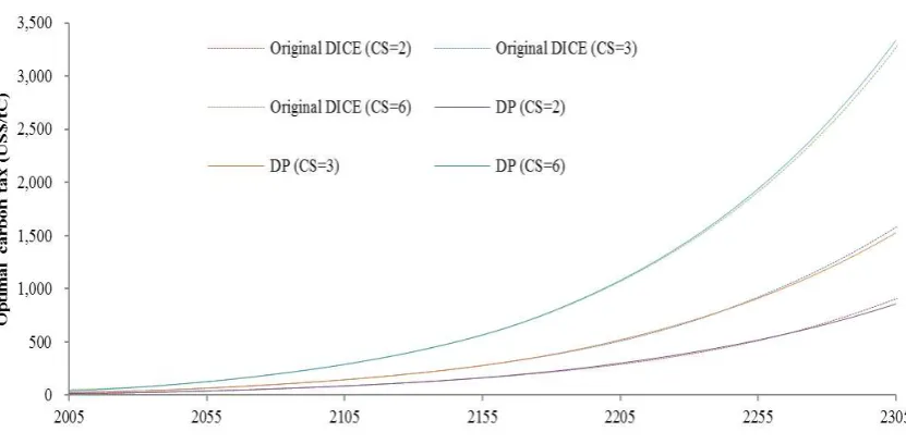
For an accuracy test, the results obtained from the deterministic version of DICE applying

the above-mentioned method in MATLAB are compared with the results obtained from the

deterministic version of DICE applying nonlinear programming in GAMS (i.e., the original

programming code, made available by William Nordhaus, is run in GAMS). Figure A.2 is the

results. It shows that the dynamic programming method produces almost the same results as

the original ones. The uncertainty model also produces good results (not shown).

In addition, the accuracy of the dynamic programming method is tested as follows. First,

the maximum welfare over a grid of the control variable is calculated every time period.22

More specifically, the model is simulated with a fixed emissions control rate (1,000 grid

points from 0 to 1) and then the rate of emissions control which results in maximum welfare

is chosen for every time period. Finally, the emissions control rate obtained above and the

emissions control rate obtained from the dynamic programming method are compared. The

result is that the maximum difference between the two values over the whole time periods is

about 10-4.

22

35 Table 1 Tail probability of the climate sensitivity distribution

Probability/Year 2005 2055 2105 2155 2205

Pro(CS>4.5℃) 0.253 0.149 0.043 0.006 4.00E-04

Pro(CS>6℃) 0.122 0.049 0.005 7.70E-05 2.98E-07

Pro(CS>10℃) 0.038 0.008 1.35E-04 6.18E-08 1.55E-12

Note: As with Figure 1, =0.65, =0.13, and =0.6 for the calculation of numbers in this table.

Table 2 The optimal carbon tax and the net present value of utility

Deterministic

=0.60

Uncertainty

=0.60, =0.13

Learning

=0.60, =0.13

LB ̅=0.55 UB ̅=0.60 HB ̅=0.65 LB =0.55 UB =0.60 HB =0.65

Optimal carbon tax in

2015 (US$/tC) 32.0 29.6 34.4 39.7 30.7 33.4 36.5

Net present value of

utility (arbitrary unit) 0 -1.711 -1.705 -1.709 -1.703 -1.703 -1.703

Note: The net present value of utility is the difference between each case and the deterministic case.

Table 3 The costs of no learning in 2105

=0.6 (true =3°C/2xCO2)

LB =0.55< =0.6 UB =0.60= =0.6 HB =0.65> =0.6 Abatement costs

(% gross world output) 0.55 0.24 0.49

Damage costs

(% gross world output) -0.20 -0.11 -0.21

Total costs

(% gross world output) 0.35 0.12 0.26

Note: The costs are calculated as the difference in the costs between the uncertainty model and the learning

36

Figure 1 Learning about the climate sensitivity (Top Left): The parameters of the climate sensitivity

distribution: the mean and the variance of the total feedback factors. (Top Right): The coefficient of variation

(= mean / standard deviation) of the simulated climate sensitivity distribution (relative to the coefficient of

variation in 2005). (Bottom Left): Climate sensitivity distribution (0~10°C/2xCO2). (Bottom Right): Climate

sensitivity distribution (10~30°C/2xCO2). The density for the year 2205 approaches 0 far faster than the other

37

Figure 2 Sensitivity of the rate of learning (Top left): Sensitivity on the true value of the climate sensitivity.

refers to the true value of the total feedback factors. The corresponding true values of the climate sensitivity

are 3°C/2xCO2 ( =0.6), 3.43°C/2xCO2 ( =0.65), and 4°C/2xCO2 ( =0.7). Throughout the top left panel

=0.65 and =0.13. (Top right): Sensitivity on the initial uncertainty. refers to the initial standard deviation of the total feedback factors. Throughout the top right panel =0.6 and =0.65. (Bottom left):

Sensitivity on temperature shocks. refers to the standard deviation of temperature shocks. (Bottom right):

Sensitivity on damage function. Throughout the bottom panels , =0.65, and =0.13.

Figure 3 The effect of learning (Top Left): Emissions control rates. (Top Right): The optimal carbon tax.

38

LRN refer to the deterministic case ( =0.6), the uncertainty case ( =0.6, ̅=0.65, =0.13), and the learning

case ( =0.6, =0.65, =0.13), respectively.

Figure 4 Carbon tax according to the initial belief (Left): The uncertainty case. FM refers to the mean of the

total feedback factors. (Right): The learning case. The relative difference in the carbon tax between the cases is

also presented in the right panel (right axis). It is calculated as follows: (the carbon tax for A - the carbon tax for

B) / the carbon tax for B, where A and B refer to each case.

Figure 5 The costs of no learning (the HB scenario) (Left): The abatement costs and the damage costs. UNC

and LRN refer to the uncertainty case and the learning case. (Right): The costs of no learning. The costs are

calculated as the difference in the costs between the uncertainty model and the learning model. Thus the positive

value means that the uncertainty case costs more than the learning case. ABT, DAM, and TOTAL refer to the

39

Figure 6 Sensitivity analysis (the HB case) (Left): The optimal carbon tax. DET, UNC and LRN refer to the

deterministic case, the uncertainty case and the learning case. The optimal carbon tax in 2015 is 373.0US$/tC

and 56.4 US$/tC for the uncertainty case and the learning case, respectively. (Right): The optimal carbon tax as

a function of uncertainty (the learning model). Note that x-axis is displayed in a logarithmic scale (base 10). In

order to reduce computational burden the standard deviation of temperature shocks are assumed to be 0.05 for

the bottom panel. This does not affect the implications of the results. Throughout the figures =0.6 (true

=3°C/2xCO2), =0.65, and =0.13.

Figure A.1 Comparison of the results from dynamic programming in MATLAB with the results from

nonlinear programming in GAMS DP refers to the results obtained from dynamic programming. Original DICE

refers to the results obtained from running the programming code made available by William Nordhaus in