On the Computing of the Minimum Distance of Linear Block Codes by Heuristic Methods

http://dx.doi.org/10.4236/ijcns.2012.511081 Published Online November 2012 (http://www.SciRP.org/journal/ijcns)

On the Computing of the Minimum Distance of Linear

Block Codes by Heuristic Methods

Mohamed Askali, Ahmed Azouaoui, Saïd Nouh, Mostafa Belkasmi SIME Lab, National School of Computer Science and Systems Analysis (ENSIAS),

Mohammed V-Souisi University, Rabat, Morocco Email: [email protected]

Received August 27, 2012; revised September 30, 2012; accepted October 8, 2012

ABSTRACT

The evaluation of the minimum distance of linear block codes remains an open problem in coding theory, and it is not easy to determine its true value by classical methods, for this reason the problem has been solved in the literature with heuristic techniques such as genetic algorithms and local search algorithms. In this paper we propose two approaches to attack the hardness of this problem. The first approach is based on genetic algorithms and it yield to good results com- paring to another work based also on genetic algorithms. The second approach is based on a new randomized algorithm which we call “Multiple Impulse Method (MIM)”, where the principle is to search codewords locally around the all-zero codeword perturbed by a minimum level of noise, anticipating that the resultant nearest nonzero codewords will most likely contain the minimum Hamming-weight codeword whose Hamming weight is equal to the minimum dis- tance of the linear code.

Keywords: Minimum Distance; Error Impulse Method; Heuristic Methods; Genetic Algorithms; NP-Hardness; Linear Error Correcting Codes; BCH Codes; QR Codes; Double Circulant Codes

1. Introduction

The Minimum distance of a linear error correcting code has a practical and theoretical interest. It provides a great deal of information on the code capability in detecting and in correcting errors or erasures.

Since, to date, these problems cannot be solved mathe- matically because it is in general a NP-hard problem, it becomes necessary to physically search the codewords of a code in order to find the codeword with the minimum weight. Unfortunately, as the size of the code increases, the size of the search space becomes prohibitively large. The number of information bits in a code, k, defines the size of a search space. Note that k is also the number of basis vectors in the code and thus the size of the search space is 2 k. Thus, an exhaustive search is not feasible, but a heuristic search may provide valuable information and, in some cases, perhaps a solution. We propose sev-eral different algorithms and heuristic search techniques such as Genetic Algorithm (GA) [1-4], and search local error using a Soft-In decoder when applied to the prob-lem of determining the true minimum distance of a linear block code [5].

In the past, many excellent studies have found the minimum weight for Quadratic Residue (QR) codes or its extended codes were presented in [6-10], in [11] we have

estimated the minimum distance of Double Circulant Codes (DCC) using genetic algorithm, and Wallis et al.

[12] have presented a different genetics techniques ap- plied to find an estimate of the minimum distance for some Bose-Chaudhuri-Hocquenghem (BCH) codes, In [13], Nouh et al. have used genetic algorithms for finding a likelihood weight enumerator of some linear block codes, in particular their minimum weights.

Other works interest to the distance measurement me- thods have been introduced: Garello’s true distance spec- trum method [14], Berrou’s error-impulse method [15], Garello’s all-zero iterative decoding method [16] and Crozier’s double (and triple) impulse method(s) [17].

Furthermore, there are also other works [18-20] based on artificial intelligence, trying to solve problems related to coding theory.

In this paper, we deal with finding a good estimate of minimum distance of linear block codes using genetic algorithms to BCH, QR, and DCC codes and which we denote dt, and we compare our results to previous works. Finally, we present results obtained by using our search local error method published in a previous work [5], where we use a Soft-In Ordered Statistics decoder (OSD).

describes the proposed heuristic methods to find a tight minimum distance, Section 4 reports the simulation re- sults and discussions. Finally, Section 5 presents the conclusion and future trends.

2. Genetic Algorithms

Genetic Algorithms was first proposed by John Holland’s, as a means to find good solutions to problems that were otherwise computationally intractable. Holland’s schema theorem [21], and the related building block hypothesis, provided a theoretical and conceptual basis for the design of efficient GA. It also proved straight forward to im- plement GA due to their highly modular nature. As a consequence, the field grew quickly and the technique was successfully applied to a wide range of practical problems in science, engineering and industry. GA the- ory is an active and growing area, with a range of ap- proaches being used to describe and explain phenomena not anticipated by earlier theory. In tandem with this, more sophisticated approaches for directing the evolution of a GA population are aimed at improving performance on classes of problem known to be difficult for GA, [21]. The development and success of GA contributed greatly to a wider interest in computational approaches based on natural phenomena. It is now a major stand of the wider field of computational intelligence, which encompasses techniques such as neural networks, and artificial immu- nology. Genetic algorithms are search methods that can be used for both solving problems and modelling evolu- tionary systems.

Since it is heuristic (it estimates a solution), GA differs from other heuristic methods in several ways. The most important difference is that it works on a population of

possible solutions, while other heuristic methods use a Another important difference is that GA is not a determi- nistic but a probabilistic one.

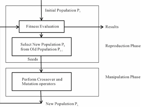
A genetic algorithm is defined by (see Figure 1): Individual or chromosome: a potential solution of the problem, it’s a sequence of genes.

Population: a set of points of the research space. Environment: the space of research.

Fitness function: the function to maximize/minimize. Encoding of chromosomes: it depends on the treated problem, the famous known schemes of coding are: bi- nary encoding, permutation encoding, value encoding and tree encoding.

Stochastic Operators:

 Selection: replicates the most successful solutions found in a population at a rate proportional to their relative quality.

 Crossover: Decomposes two distinct solutions and then randomly mixes their parts to form novel solu- tions.

 Mutation: Randomly perturbs a candidate solution. In the selection process, some individuals are selected to be copied into a tentative next population. Individ-ual with higher fitness value is more likely to be se-lected. The selected individuals are altered by the mutation and crossover and form a new population of solutions. The GA is simple yet provides an adaptive and robust optimization methodology [22].

3. Estimation Methods for Finding the

Minimum Distance

3.1. Methods Based on Genetic Algorithms

In the sequel of this paper, we use the following nota-

tions:

 Ni the cardinal of the population.

 Coding the encoding function.

 Ng the number of generations.

 Ne the number of elites (better parents).

 Ngmax is the maximum number of generations and C(I) is the codeword obtained by coding the information vector I.

In order to use genetic algorithms, in our work, we use binary encoding which consists to treat an individual as a binary sequence. We proposed Two GA variants A and B.

3.1.1. Genetic Algorithm: Variant A

This algorithm permits to find a minimum weight in a linear code C. It is known in field of coding theory that there exists always a linear systematic code equivalent to C. For the purposes of this paper we suppose that the generator matrix G of the code C is systematic; this chose permits to initialize the initial population by words of weight less than the global upper bound corresponding to the length n and the dimension k. the algorithm ex- pects as inputs the probability of mutation pm of a single

bit, and the crossover probability pc.

 Algorithm Steps

The steps of the algorithm are organized as follow: Step 1: randomly generate an initial population

Seed uniformly, randomly the initial population with a Ni, and where each individual is a word of length k with

a random weight. We initiate the number of generation Ng to 1.

Step 2: while (Ng < Ngmax)do

Step 2.1: Compute the fitness of each individual in the population

An individual i represents an information vector of k bits which is encoded by the code generator to an n-bit code vector. The fitness is the weight of the encoded in- dividual if this last is different to zero otherwise, the fit- ness is equal to n as a maximum value.







( 0)

dividual

f if f n otherwise





p p



p p







f weight Coding in

fitness individual



   

Step 2.2: Sort population in increasing order of fit- ness

Step 2.3: Insert the best Ne = 50% individuals in the intermediate population

Step 2.4: For i = Ni/2 to Ni

Step 2.4.1: Randomly select two individuals p1 and p2 for reproduction

Step 2.4.2: 1 = mutate (p1) and 2 = mutate (p2): Flip each bit of p1 and p2 with probability pm

Step 2.4.3: Cross ( 1, 2) with probability pc to pro- duce two children ch1 and ch2

Step 2.4.4: f1 weight (Coding (ch1)); f2 weight (Coding (ch2))

Step 2.4.5: if (f1 < f2) then insert ch1 in the interme- diate population else insert h2

End For End while

Step 3: output the first individual in the last popula- tion

 Description of the Algorithm

In this entire paper, the crossover and the mutation stochastic operators operate only on the information bits represented as k-dimensional vectors. An alternative strategy is to represent individuals as n bit codewords.

In Step 2.1, to evaluate the fitness of an individual, it is necessary to first encode it by multiplying it with gen- erator matrix G or by the generator polynomial if the code is cyclic as in some cases of our study. If the weight of the encoded vector is not null, the fitness is equal to weight (Coding (vector)) otherwise the fitness is equal to n. An individual is better than another if its weight is the smallest.

In Step 2.2 and Step 2.3, we use a Linear Ranking Se- lection strategy where individuals in population are sorted by non-decreasing order of weight of encoded individual vector, and we select the best Ne = 50% indi-

viduals to yield the intermediate population.

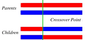
In Step 2.4, we use a single crossover point strategy, in which both parents organism strings is selected. All data beyond that point in either organism string is swapped between the two parents organisms. The result- ing organisms are the children (see Figure 2).

Concerning selection, we use the random selection, in that only Ne individuals are preserved in the next genera- tion, and we select randomly two parents to reproduce a best offspring that is more likely to contain good schema. The mutation step is done bit-wise on offspring with probability pm.

3.1.2. Genetic Algorithm: Variant B

 Algorithm Steps

The steps of the algorithm are organized as follow: Step 1: randomly generate an initial population

Seed uniformly, randomly the initial population with a Ni, and where each individual is a word of length k with

a random weight. We initiate the number of generation Ng to 1.

Parents

Children

Crossover Point

Step 2: while (Ng < Ngmax) do

Two point Crossover Parents

Children

Uniform Crossover

Step 2.1: Compute the fitness of each individual in the population

An individual i represents an information vector of k bits which is encoded by the generator code to an n-bit code vector. The fitness is the weight of the encoded in- dividual if this last is different to zero otherwise, the fit- ness is equal to n as a maximum value.









f weight Coding individual

Step 2.2: Sort population in increasing order of fitness Step 2.3: select the best Ne individuals in the inter- mediate population

Step 2.4: i = Ne to Ni

Step 2.4.1: tournament select of two parents p1 and p2 for reproduction

Step 2.4.2: If (rand_value < pc) {Cross p1 and p2 to generate ch1 and ch2; Mutate ch1 and ch2 and introduce them in the next population} Else introduce p1 or p2 into the next population with equal probability.

End For

Step 2.5: Let currbest = fittest of the intermediate population. If (fitness (best) < fitness (currbest)) best = currbest

End while

Step 3: output best

 Description of the Algorithm

There are many differences between variant A and this variant in strategies of selection, order of stochastic op- erators, and the method of offspring reproduction.

In Step 2.4.1, we use the tournament selection, in that only one of two possible parents is preserved to repro- duce two children whose will be inserted in the next generation.

Step 2.4.2, in this variant, the crossover operation de- pends on pc, and it is done before the mutation step

which is done bit-wise on offspring with probability pm.

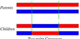
In case of no-cross we insert the two initials parents in the next generation. We have used three strategies of crossover: a single crossover point (depicted in Figure 2), two point crossover, and uniform crossover. The two- point Crossover that randomly selects two crossover points within a chromosome then interchanges the two parent chromosomes between these points to produce two new offspring (see Figure 3). The Uniform Cross- over uses a fixed mixing ratio between two parents. Unlike one- and two-point crossover, the Uniform Cross- over enables the parent chromosomes to contribute the gene level rather than the segment level. An example of this operation is depicted in Figure 4.

3.2. A New Algorithm Based on Error Impulse Method

This method is not based on the analysis properties of the

Figure 3. Two-point crossover structure.

Parents

Children

Figure 4. Uniform crossover structure.

code but on the correction capability of the decoder. To obtain a good estimate of the minimum distance of a code, it is critical to apply a noise as possible to the all-zero codeword, so that the noise energy brings the decoder marginally away from the all-zero codeword.

The nature of the noise is so important, and it depends on the decoder used, for this, Berrou has proposed in [15] the Error impulse Method to excite the MLD decoder for turbo codes, and Xiao et al. [23] has proposed the Bit Reversing to excite the iterative decoder IRB proposed by Fossorier for LDPC codes. Another recent approach, by Garello et al. [24], is called the “all-zero iterative de- coding algorithm”. Here, this approach will be referred to as the “single impulse method” for reasons that will be- come apparent. This approach is similar to the error im- pulse method in that an impulse is again placed at a spe- cific data index in the all-zero codeword. The main dif- ference is that the amplitude of the impulse is intention- ally set very high so that the decoder cannot correct it, but rather is forced to converge to (or at least select) a non-zero data pattern.





We denote by        the word as- sociated to the “all-zero” codeword modulated by the BPSK.

3.2.1. Berrou’s Algorithm

The noise pattern proposed by Berrou et al. in [15] called Error Impulse, which was originally proposed for com- puting the minimum distance of Turbo codes.

the all-zero codeword at a specific data index to see if the Turbo decoder can correct it. The amplitude of the error impulse is increased until the decoder fails. The highest amplitude that could be corrected provides an estimate of the minimum distance associated with that specific data index. An estimate of the overall minimum distance is obtained by testing all of the data indices in this manner. It was shown in [15] that this approach is guaranteed to find the true dt if the decoder is a true maximum likely-

hood (ML) decoder. Of course, Turbo decoders are not true ML decoders. Thus, there is no guarantee that the error impulse method will find the true dt. Further, al-

though this approach is usually pessimistic, there is no guarantee that the result will be a true lower bound on dt.

3.2.2. The Proposed Multiple Impulse Method (MIM) The proposed algorithm produces a tight minimum dis- tance based on true (low-weight) codewords found by a fine-tuned local search.

We assume that dt is in the range [d0, d1] where d0 and d1 are two integers. Then dt can be determined as follows:

Step 1: set Amin = d1 + 0.5 and dt = n − k1; nb_test. Step 2: For i = 1 to nb_test

Step 2.1: A = d0 – 0.5;

Step 2.2: Set [(x=x) = TRUE]; =

 x

 x

 

=

 x x

i

Step 2.3: While [(x ) = TRUE] & [A ≤ Amin – 1.0] Step 2.3.1: A = A + 1.0

Step 2.3.2: For nb_error = error_max to 1

Step 2.3.3: Subdivide A randomly on nb_error posi- tions

Step 2.3.3.1: OSD decoding of Y 

Step 2.3.3.2: If (weight (x)≤ dt) then dt = weight (x) Step 2.3.3.3: If (x=x) then [( ) = TRUE] End for

End while

Step 2.4: Amin = A; End for

Output: dt is the minimum distance

We changed the Soft-In MLD decoder used in Ber-rou’s [15] Algorithm by a Soft-In OSD decoder which is very fast, by injecting a noise iteratively in a random positions, the decoder word will be mostly near than the “all-zero” codeword, and the minimum distance of the code will be the minimum weight of the decoded words and is not the magnitude A of the noise as we have in Error Impulse Method.

4. Results and Discussions

4.1. Parameters Optimization of Genetic Algorithms

In Tables 1-4, we analyze the impact of genetic opera- tors on the minimum distance.

Table 1. Effect of elitism operator.

Minimum distance Codes

Without elitism With elitism

BCH (255, 99, 47) 58 52

BCH (255, 107, 45) 53 53

BCH (255, 115, 43) 46 46

QR (193, 97, 27) 28 27

QR (199, 100, 31) 35 31

QR (223, 112, 31) 36 32

Table 2. Effect of crossover operator types.

Minimum distance Codes

1-point 2-point Uniform

BCH (255, 99, 47) 58 52 57

BCH (255, 107, 45) 51 53 52

BCH (255, 115, 43) 48 46 46

QR (193, 97, 27) 30 27 30

QR (199, 100, 31) 31 31 32

QR (223, 112, 31) 35 32 35

Table 3. Effect of selection types.

Minimum distance Codes

Tournament Random Roulette

BCH (255, 99, 47) 52 53 53

BCH (255, 107, 45) 53 50 53

BCH (255, 115, 43) 46 46 46

QR (193, 97, 27) 27 30 30

QR (199, 100, 31) 31 31 31

QR (223, 112, 31) 32 35 32

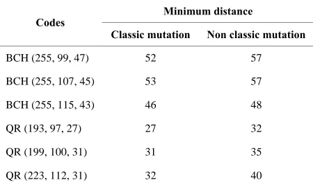
Table 4. Effect of mutation operator types.

Minimum distance Codes

Classic mutation Non classic mutation

BCH (255, 99, 47) 52 57

BCH (255, 107, 45) 53 57

BCH (255, 115, 43) 46 48

QR (193, 97, 27) 27 32

QR (199, 100, 31) 31 35

4.1.1. Effect of Elitism

It appears that elitism significantly improves the per- formance of genetic algorithm for QR codes and BCH codes.

4.1.2. Effect of Crossover

These results explain that 2-point crossover seems to perform significantly better than uniform and 1-point crossover for QR codes and BCH codes.

4.1.3. Effect of Selection

As shown results in the Table 3, in general, the tourna- ment selection gives a very close upper bound to the minimum distance for QR codes and BCH codes.

4.1.4. Effect of Mutation

In this paragraph, we compare the impact of the classic mutation with other type of mutation. This last alters an individual by bit inversion of chromosome. However, such an inversion takes place only in one bit and only when an improvement in the individual’s fitness is achieved. If it is not possible to improve the individual‘s fitness, then no alteration is performed. The algorithm simply goes through every chromosome’s gene to deter- mine which of them must be changed in such a way as to

improve individual’s fitness.

According to the results of this study, we concluded that the best parameters for this algorithm are: Elitism operator, tournament selection, 2-point crossover, and classical mutation.

4.2. Results of Various Genetic Algorithms

All simulations were made with default GA parameters outlined in the Table 5.

The Table 6 shows that the proposed algorithms out-

Table 5. Parameters of implementation of genetic algo-rithms.

Parameter Wallis’s GA GA-A GA-B

Probability of Crossover 80% 93% 80%

Probability of Mutation 2% 1% 2%

Crossover Type 2-point 1-point 2-point

Selection Type Tournament Random Tournament

Tournament Size 3 - 2

Generation Number 75 75 75

Individuals Number 10,000/1000 10,000/1000 10,000/1000

Table 6. Comparaison of our GA algorithms with other works for some BCH codes.

Codes BCH (n, k, d-design)

dt GA-A 10000

individuals

dtGA-B 10000

individuals Wallis’s GA Hill-Climbing Tabu Search

BCH (127, 64, 21) 21 21 21 28 24

BCH (127, 57, 23) 23 23 23 28 23

BCH (127, 50, 27) 27 27 27 32 31

BCH (255, 71, 59) 64 63 66 79 79

BCH (255, 79, 55) 57 57 60 74 64

BCH (255, 87, 53) 57 58 57 70 66

BCH (255, 91, 51) 58 53 59 72 69

BCH (255, 99, 47) 51 52 55 64 61

BCH (255, 107, 45) 53 49 51 64 62

BCH (255, 115, 43) 48 45 50 57 55

BCH (511, 304, 51) 87 74 79 90 85

BCH (511, 286, 55) 98 84 84 96 92

BCH (511, 238, 75) 113 103 105 118 112

BCH (511, 220, 79) 112 109 111 123 117

BCH (511, 184, 91) 111 127 128 135 140

BCH (511, 166, 95) 143 135 137 152 140

BCH (511, 121, 117) 159 155 152 163 163

BCH (511, 103, 123) 164 160 164 179 179

BCH (511, 76, 171) 176 176 176 195 184

performed the other optimization techniques.

The Table 7 shows the computational results of mini- mum distance via GA-A, GA-B, and the Simulated An- nealing (SA) developed by authors in [25].

In the Table 7, for the three first BCH codes listed, these algorithms found the true minimum distance. However, for the two last BCH codes, the gap between the minimum distance obtained by the SA algorithm and the true value is still large, while our genetic algorithms found this true minimum distance.

The Table 8 shows that our two variants of GA give the same estimate of the minimum distance for Quadratic residue codes where the length is less than 223.

The Table 9, we validate our estimate minimum dis- tance by the exhaustive method for some random DCC defined by their binary header.

Table 7. Comparaison between our two GA variants with simulated annealing.

Codes BCH (n, k, d-design)

dt GA-A 10000

individuals

dt GA-B 10000

individuals

Simulated annealing

BCH (15, 11, 3) 3 3 3

BCH (31, 26, 3) 3 3 3

BCH (63, 24, 15) 15 15 15

BCH (127, 64, 21) 21 21 27

BCH (255, 91, 51) 51 51 75

Table 8. Comparaison between our two variants applied to QR codes.

Codes QR (n, k, d)

dtGA-A 1000

individuals

dt GA-B 1000

individuals

QR (47, 24, 11) 11 11

QR (71, 36, 11) 11 11

QR (73, 37, 13) 13 13

QR (79, 40, 15) 15 15

QR (89, 45, 17) 17 17

QR (97, 49, 15) 15 15

QR (113, 57, 15) 15 15

QR (127, 64, 19) 19 19

QR (137, 69, 21) 21 21

QR (151, 76, 19) 19 19

QR (191, 96, 27) 27 27

QR (193, 97, 27) 30 30

QR (199, 100, 31) 31 31

QR (223, 112, 31) 32 32

4.3. Validation and Results of Multiple Impulse Method

4.3.1. Validation of the Multiple Impulse Method All simulations have been done using a simple configu- ration machine: Intel® CoreTM 2 CPU T5600 @ 1.83 GHz, RAM: 2.00 GHz.

As a first step, we validated the algorithm by verifying the minimum distance for some linear codes: BCH codes, Quadratic residue Codes, and Quadratic Double-Circu- lant Codes in their Bordered form, for which the mini- mum distance is known.

The results are summarized in the Tables 10-12, in which “OSD_EI” denotes the Order Statistic Decoding with Error impulse and “TTE” denotes the Time of exe- cution in seconds. As it is shown in these tables our algo- rithm is successfully validated.

Let p be a prime that is congruent to ±3 modulo 8. A binary [2(p + 1), p + 1] quadratic double-circulant code (QDC) [26], denoted by B, can be constructed using the following defining polynomials:

 









1+ if p 3 mod 8 and

if p 3 mod 8

r r Q

r r Q

x b x

x





 



  _{ }







2

.

d n

(1)

Q is the set of quadratic residues modulo p.

The generator matrix G of B can be written as de- scribed in Figure 5.

We find exactly what Tomlinson has found in [26].

4.3.2. New Experimental Results

In this section we present an application of the proposed algorithm to find the true unknown minimum distance of some residue quadratic codes (QR and QDC see Tables 14-16) and some BCH codes (see Table 13) comparing respectively to some known upper bounds, and to the designed distance or comparing to the Grassl table [27].

By MacWilliams and Sloane in [28], for QR codes, we compare our estimation by this inequality

By the Pless’s identity [29], the minimum weight in Quadratic Residue codes is always odd. This means that when we find a codeword with a pair weight w, it is nec- essary to have a codeword with an odd weight w-1.

In the Table 14 we give some QR codes where the length is like the form n = 8 m + 1.

In our knowledge the Krasikov Bound [30] is the best upper bound for comparing our estimation of the mini-mum distance.In the Table 15 we give some QR codes

1 0

1 0

0 0 0 1 1 1

p

I B

G  

 

Table 9. Comparaison between our two variants applied to QR codes.

Double Circulant

Codes (DCC) Binary Header of DCC

dt Our GA-A

1000 Individuals

dt Our GA-B

1000 Individuals Exhaustive Method

C (20, 10) 1001111110 6 6 6

C (22, 11) 00010110111 7 7 7

C (24, 12) 101000110111 8 8 8

C (26, 13) 1000100111100 7 7 7

C (28, 14) 00101001111111 8 8 8

C (30, 15) 001110111111101 8 8 8

C (32, 16) 1010100100100110 8 8 8

C (34, 17) 10011001011010011 8 8 8

C (36, 18) 101000100011111111 8 8 8

C (38, 19) 110010000011111101 8 8 8

C (40, 20) 000111001100110101011 9 9 9

C (42, 21) 000101111011110011110 10 10 10

C (44, 22) 1100011101010101001111 10 10 10

C (46, 23) 01101101111101011110000 11 11 11

C (50, 25) 1001000111111001011000000 10 10 10

C (52, 26) 11000100110110001110110010 10 10 10

C (54, 27) 011000110000111111101101000 11 11 11

C (58, 29) 00011011111000110010010010010 12 12 12

C (62, 31) 1100001010100011100000011010110 12 12 12

Table 10. Validation of some QR codes with known mini- mum distance.

Codes QR (n, k, d) dt OSD_EI TTEs

QR (41, 21, 9) 9 1.12

QR (47, 24, 11) 11 0.61

QR (71, 36, 11) 11 0.71

QR (73, 37, 13) 13 0.75

QR (79, 40, 15) 15 1.29

QR (89, 45, 17) 17 3.66

QR (97, 49, 15) 15 0.99

QR (113, 57, 15) 15 4.23

QR (127, 64, 19) 19 11.08

QR (137, 69, 21) 21 14.33

QR (151, 76, 19) 19 33.01

QR (191, 96, 27) 27 213

QR (193, 97, 27) 27 220

QR (199, 99, 31) 31 145

QR (223, 112, 31) 31 124

where the length is like the form n = 8m − 1, and we have: d0.166315 n.

For the class of QDC codes we give in the next table some codes with unknown minimum.

Table 11. Validation of some BCH codes with known mini- mum distance.

Codes BCH (n, k, d-design) dtOSD_EI TTEs

BCH (31, 16, 7) 7 0.02

BCH (31, 21, 5) 5 0.01

BCH (63, 18, 21) 21 0.04

BCH (63, 24, 15) 15 0.06

BCH (63, 36, 11) 11 0.07

BCH (63, 39, 9) 9 0.05

BCH (63, 30, 13) 13 0.04

BCH (63, 45, 7) 7 0.06

BCH (63, 51, 5) 5 0.05

BCH (63, 57, 3) 3 0.01

BCH (127, 8, 63) 63 0.67

BCH (127, 15, 55) 55 0.7

BCH (127, 22, 47) 47 0.37

BCH (127, 29, 43) 43 0.51

BCH (127, 71, 19) 19 2.85

BCH (127, 78, 15) 15 2.08

BCH (127, 92, 11) 11 1.37

BCH (127, 106, 7) 7 0.74

BCH (255, 45, 87) 87 57

Table 12. Validation of some QDC codes with known mini- mum distance.

Codes QDC

(2(p + 1), p + 1, d) dt OSD_EI TTEs

QDC (24, 12, 8) 8 0.97

QDC (28, 14, 8) 8 1.02

QDC (40, 20, 8) 8 1.4

QDC (60, 30, 12) 12 2.86

QDC (76, 38, 12) 12 6.61

QDC (88, 44, 16) 16 9.88

QDC (108, 54, 20) 20 34.98

QDC (120, 60, 20) 20 33.33

QDC (124, 62, 20) 20 33.18

QDC (136, 68, 24) 24 57

QDC (168, 84, 24) 24 1052

Table 13. Tight bound for unknown minimum distance of some BCH codes.

Codes BCH

(n, k, d-design) dt OSD_EI TTEs

BCH (127, 64, 21) 21 10

BCH (127, 57, 23) 23 1

BCH (127, 50, 27) 27 4

BCH (255, 71, 59) 62 530

BCH (255, 79, 55) 55 631

BCH (255, 87, 53) 53 5915

BCH (255, 91, 51) 51 7617

BCH (255, 115, 43) 43 8283

BCH (255, 123, 39) 39 7098

BCH (255, 131, 37) 37 7570

BCH (255, 139, 31) 31 7051

BCH (255, 147, 29) 29 4626

BCH (255, 155, 27) 27 4177

BCH (255, 163, 25) 25 2612

BCH (255, 171, 23) 23 2847

BCH (255, 179, 21) 21 1653

BCH (255, 187, 19) 19 65

BCH (255, 191, 17) 17 1198

BCH (255, 199, 15) 15 384

Table 14. Tight bound of the unknown minimum distance of some QR codes.

Codes QR Square (n) dtOSD_EI TTEs

n = 233 k = 117 15.26 25 198

n = 241 k = 121 15.52 31 835

n = 257 k = 129 16.03 33 5851

n = 281 k = 141 16.76 35 40435

n = 313 k = 157 17.69 45 51498

n = 337 k = 169 18.35 51 45539

Table 15. Tight bound of the unknown minimum distance of some QR codes.

Codes QR Krasikov _bound dt OSD_EI TTEs

n = 239 k = 129 39.74 31 308

n = 263 k = 132 43.74 35 66173

n = 271 k = 136 45.07 39 65659

n = 311 k = 156 51.72 35 62286

n = 359 k = 180 59.70 55 60621

n = 367 k = 184 61.03 59 74650

n = 383 k = 192 63.69 59 81810

n = 431 k = 216 71.68 67 101409

n = 439 k = 220 73.01 71 90579

Table 16. Tight bound of the unknown minimum distance of some QDC codes.

Codes QDC

(2(p + 1), p + 1) dtOSD_EI TTEs

QDC (204, 102) 24 5886

QDC (216, 108) 24 1421

QDC (220, 110) 30 7595

QDC (264, 132) 40 27547

QDC (280, 140) 36 24683

QDC (300, 150) 44 28371

QDC (316, 158) 46 35892

QDC (328, 164) 48 53135

5. Conclusion and Perspectives

competitor genetic algorithm developed by Wallis. For the same goal, we have proposed the Multiple Impulse Method based on Soft-In OSD decoding algo- rithm by generalization of the method proposed initially by Berrou et al. The MIM technique is highly performing as a good tool for computing the minimum distance of linear codes, especially for a large code where the length is so long. In the perspectives of this work, we have to apply these powerful tools to construct good linear block codes, and to test the effect of other Soft-In decoders in terms of complexity and performances.

REFERENCES

[1] H. Chen, N. S. Flann and D. W. Watson, “Parallel Ge- netic Simulated Annealing: A Massively Parallel SIMD Algorithm,” IEEE Transactions on Parallel and Distrib- uted Systems, Vol. 9, No. 2, 1998, pp. 126-136.

doi:10.1109/71.663870

[2] C. Cotta, E. Alba and J. M. Troya, “Utilising Dynastically Optimal Forma Recombination in Hybrid Genetic Algo-rithms,” In: A. Eiben, T. BÄack, M. Schoenauer and H. Schwefel, Eds., Parallel Problem Solving from Nature, Springer-Verlag, Berlin, 1998, pp. 305-314.

[3] J. M. Daida, S. J. Ross and B. C. Hannan, “Biological Symbiosis as a Metaphor for Computational Hybridiza-tion,” In: L. Eshelman, Ed., Proceedings of the 6th Inter-national Conference on Genetic Algorithms, Pittsburgh, 15-19 July 1995, pp. 328-335.

[4] K. Dontas and K. De Jong, “Discovery of Maximal Dis-tance Codes Using Genetic Algorithms,” Proceedings of the 2nd International IEEE Conference on Tools for Arti-ficial Intelligence, IEEE Computer Society Press, Los Alamitos, 1990, pp. 905-811.

[5] M. Askali, S. Nouh and M. Belkasmi, “An Efficient Method to Find the Minimum Distance of Linear Block Codes,” IEEE International Conference on Multimedia Computing and Systems Proceeding, Tangier, 10-12 May 2012, pp. 185-188.

[6] D. Coppersmith and G. Seroussi, “On the Minimum Dis-tance of Some Quadratic Residue Codes,” IEEE Transac-tions on Information Theory, Vol. 30, No. 2, 1984, pp. 407-411. doi:10.1109/TIT.1984.1056861

[7] N. Boston, “The Minimum Distance of the [137, 69] Quadratic Residue Code,” IEEE Transactions on Infor-mation Theory, Vol. 45, No. 1, 1999, p. 282.

doi:10.1109/18.746813

[8] D. Kuhlmann, “The Minimum Distance of the [83, 42] Quadratic Residue Code,” IEEE Transactions on Infor-mation Theory, Vol. 45, No. 1, 1999, p. 282.

doi:10.1109/18.746814

[9] Markus Grassl, “On the Minimum Distance of Some Quadratic Residue Codes,” Proceedings IEEE Interna-tional Symposium on Information Theory, Sorrento, 25-30 June 2000.

[10] W.-K. Su, P.-Y. Shih, T.-C. Lin and T.-K. Truong, “On the Minimum Weights of Binary Extended Quadratic

Residue Codes,” Proceedings of the 11th International Conference on Advanced Communication Technology, Vol. 3, IEEE Press, Piscataway, 2009.

[11] A. Azouaoui, M. Askali and M. Belkasmi, “A Genetic Algorithm to Search of Good Double-Circulant Codes,” IEEE International Conference on Multimedia Comput-ing and Systems ProceedComput-ing, Ouarzazate, 7-9 April 2011, pp. 829-833.

[12] J. Wallis and K. Houghten, “A Comparative Study of Search Techniques Applied to the Minumum Distance of BCH Codes,” Conference on Artificial Intelligence and Soft Computing, Banff, 17-19 July 2002.

[13] S. Nouh and M. Belkasmi, “Genetic Algorithms for Find-ing the Weight Enumerator of Binary Linear Block Codes,” International Journal of Applied Research on Information Technology and Computing, Vol. 2, No. 3, 2011, pp. 557-568.

[14] R. Garello, P. Pierleoni and S. Benedetto, “Computing the Free Distance of Turbo Codes and Serially Concatenated Codes With Interleavers: Algorithms and Applications,” IEEE Journal on Selected Areas in Communications, Vol. 19, No. 5, 2001, pp. 800-812. doi:10.1109/49.924864

[15] C. Berrou, S. Vaton, M. Jezequel and C. Douillard, “Computing the Minimum Distance of Linear Codes by the Error Impulse Method,” Proceedings of IEEE Globe-com, Taipei, 17-21 November 2002, pp. 10-14.

[16] R. Garello and A. Vila, “The All-Zero Iterative Decoding Algorithm for Turbo Code Minimum Distance Computa-tion,” IEEE International Conference on Communica-tions, Paris, 20-24 June 2004, pp. 361-364.

[17] S. Crozier, P. Guinand and A. Hunt, “Computing the Minimum Distance of Turbo-Codes Using Iterative De- coding Techniques,” Proceedings of 22nd Biennial Sym- posium on Communications, Kingston, Ontario, 31 May-3 June 2004, pp. 306-308.

[18] P. Praveenkumar, R. Amirtharajan, K. Thenmozhi and J. B. B. Rayappan, “Regulated OFDM-Role of ECC and ANN: A Review,” Journal of Applied Sciences, Vol. 12, No. 4, 2012, pp. 301-314. doi:10.3923/jas.2012.301.314

[19] R. Sujan, et al., “Adaptive ‘SOFT’ Sliding Block Decod- ing of Convolutional Code Using the Artificial Neural Net-Work,” Transactions on Emerging Telecommunica-tions Technologies, Vol. 23, No. 7, 2012, pp. 672-677.

doi:10.1002/ett.2523

[20] A. Azouaoui, M. Belkasmi and A. Farchane, “Efficient Dual Domain Decoding of Linear Block Codes Using Genetic Algorithms,” Journal of Electrical and Computer Engineering, Vol. 2012, 2012, Article ID: 503834.

doi:10.1155/2012/503834

[21] K. Dontas and K. Dejong, “Discovery of Maximal Dis-tance Codes Using Genetic Algorithms,” Proceedings of the 2nd International IEEE Conference on Tools for Arti-ficial Intelligence,Herndon,6-9 November 1990.

[22] D. Coley, “An Introduction to Genetic Algorithms for Scientists and Engineers,” World Scientific, Singapore City, 1999.

Parity-Check Codes,” IEEE International Conference on Communications, Paris, 20-24 June 2004, pp. 767-771. [24] R. Garello and A. Vila, “The All-Zero Iterative Decoding

Algorithm for Turbo Code Minimum Distance Computa- tion,” IEEE International Conference on Communica- tions, Paris, 20-24 June 2004, pp. 361-364.

[25] M. Zhang and F. Ma, “Simulated Annealing Approach to the Minimum Distance of Error-Correcting Codes,” In-ternational Journal of Electronics, Vol. 76, No. 3, 1994, pp. 377-384.

[26] C. Tjhai, M. Tomlinson, R. Horan, M. Ahmed and M. Ambroze, “Some Results on the Weight Distributions of the Binary Double Circulant Codes Based on Primes,” Proceedings of 10th IEEE International Conference on

Communication Systems, Singapore City, 30 October-1 November 2006.

[27] M. Grassl, IAKS, “Fakultät für Informatik,” Universität Karlsruhe, Karlsruhe, 2006.

[28] F. J. McWilliams and N. J. A. Saloane, “The Theory of Error-Correcting Codes,” North Holland, Amsterdam, 1977.

[29] V. Pless, et al., “Handbook of Coding Theory,” North Holland, Amsterdam, 1998.

[30] I. Krasikov and S. Litsyn, “An Improved Upper Bound on the Minimum Distance of Doubly-Even Self-Dual Codes,” IEEE-IT, Vol. 46, No. 1, 2000, pp. 274-278.