Parametrization procedure solution of optimal control problems over spline spaces

OPTIMAL CONTROL PROBLEMS OVER SPLINE SPACES

A Thesis presented for the degree of

Doctor of Philosophy in Electrical Engineering

in the

Uni versity of Canterbury.

Christchurch. New Zealand.

by

F. S. Chou, B.Sc. (Hons.)

l , _ /

ACKNOWLEDGEMENTS

For his patient guidance and invaluable advice throughout the

period of this research, I am deeply indebted to my thesis supervisor,

Dr. H. R. Sirisena.

I would like to thank the University Grants Committee of New

Zealand for the award of a Postgraduate Scholarship.

Finally, I wish to thank Miss B. V. Nottingham for typing the

CHAP'rER 1

1.1 1.2

1.3

1.4

CHAP'rER 2

2.1 2.2 2.3 2.4 2.5 2.6

2.7

CHAPTER 3

3.1 3.2 3.3 3.4 3.5 INTRODUCTION

Numerical Methods for Optimal Control Problems

The Ha<thematical Programming Approach

Distributed Parameter Systems

Thesis Organization

References

THE CONTROL PARAMETRIZATION PROCEDURE

Introduction

Review of Spline Functions

Problems without Constraints

Problems with Terminal Constraints

Problems with Control Constraints

Problems with State Constraints

conclusions

References

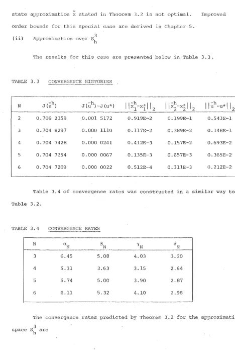
- ERROR BOUNDS FOR THE CON'l'ROL PARAME'l'RIZ.ATION

PROCEDURE

Introduction

Unconstrained Problems - Linear Quadratic Case

Unconstrained Problems - General Case

Problems with Fixed Terminal State

4.2

4.3

4.4

4.5

CHAP'rER 5

5.1 5.2 5.3 5.4 5.5 5.6

CHAPTER 6

6.1 6.2 6.3 6.4 6.5 6.6

The SP Procedure for General Control Problems The SP Procedure for a Class of

P:t:oblems

Problems with Linear Constraints Conclusions

References

Control

ERROR BOUNDS FOR THE STA'rE PARAMETRIZATION PROCEDURE

Introduction

The Ritz Procedure

Linear Quadratic Problems Multivariable System Problems Nonlinear Problems

Conclusions References

- THE S'l'ATE PARM1ETRlZATION PROCEDURE FOR DISTRIBUTED P ARANETER SYS'rEHS

In"troduction

Classification of Distributed Systems Multivariate Spline Functions

APPENDIX A

B

l' .. PPENDIX C

References

MATHEMATICAL BACKGROUND

A SUMM.i\RY OF PARAMETRIZATION PROCEDURES

SOLUTION OF A BOUNDARY CONTROL PROBLEM

137

138

142

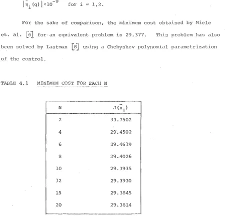
In this thesis we report on investigations into the numerical

solution of deterministic, continuous-time optimal control problems via

parametrization techniques. These methods involve the linear expansion

of one or more problem variables (Le. control, state, co-state) in terms

of functions. In this way the original optimal control problem

c2m be reduced -to a finite-dimensional minimization problem which may be

solved numerically using standard mathematical prograrruning algorithms.

Two specific techniques are considered here; we refer to them as

the control pa.rametrization (CP) and the state parametrization procedures

(SP) . As their names imply, the CP and SP procedures involve the

expansion of the control and state, respectively, in terms of basis

functions.

The importance of splines in the interpolation and approximation

of functions is well known. In this research the viability of employing

splines in conjunction with the above mentioned parametrization procedures

is examined. The rates of convergence of the CP and SP solutions are

also analysed; under smoothness conditions, explicit error

bounds are derived for the control, state and cost functional convergences._

Numerical results supporting the validity of these error bounds are

presented.

All the numerical computations in this research have been done on

the University of Canterbury Burroughs 6700/7700 machine using

u

inf

sup

T

x

Ixl

Ilx II

x

Dn X,X (n)

a

S

h

Is an element of

Is a subset of

Union

Intersection

Infimmu, or greatest lower bound

, or least upper bound

n-dimensional Euclidean space

of x.

Euclidean inner product of x and y.

Modulus of

x

Norm of X

Derivative of x with to time t. nth-derivative of x with to time t.

of functions with continuous ath order derivatives

on

of functions with continnous ath order

derivatives.

CHAPTER 1

INTRODUC'rION

1.1 NUMERICAL METHODS FOR OPTIMAL CONTROL PROBLEMS

The two or advances in modern control theory have been ( a) the

dynamic _{approach of Bellman [lJ based upon the} of

and (b) the maximum principle of Pontryagin

[2J

is an extension of the classical calculus of variations.

The main result of the dynamic programming approach to the continuous

time control problem is the Hamilton-Jacobi-Bellman

for the

differential

return function. In general this is a nonlinear part.ial

which is extremely difficult to solve

However, in those special cases when a closed form solution to the HJB

can be found, the optimal control is obtained as a feedback law;

that is, the optimal control is determined as a function of the state.

The programming technique was originally deve for discrete

time control problems. For these problems, application of the

results in a set of recursive relations which can be conveniently

solved on a digital computer. The chief drawback of programming

is its enormous computer storage requireYt1ents. This has been

overcome by the state increment algorithm of Larson

In comparison to dynamic programming, the maximum of

a more popular approach to the numerical solution of the

control problem. Numerical methods based on the maximum principle

can be classified as one of two types. The first includes

all ·the so-called indirect methods which are based on l:he t,vo point

of the maximum principle to the optimal control problem. Some of the

better known techniques belonging to this category are described below.

(1) Quasilinearization [4J: 'rhis method the nonlinear 'rPBVP by a sequence of linear boundary value problems which can be solved

'1'he major drawback of this method is that a good initial guess of the

solution is usually necessary for convergence. However, if the method

converges, i t does so quadratically to the solution.

(2) Invariant imbedding [5]: This procedure imbeds the TPBVP within a

class of more general initial value problems.

(3) Shooting method [6]: This method iterates on the initial values

of the costate variables, leaving their terminal conditions unsatisfied

until the solution is obtained. The main difficulty with this approach

lies in -the fact that boundary conditions are highly sensitive to small

changes in initial conditions because the state-costate system of equations

is inherently unstable.

The second category of numerical methods are the so-called direct

.methods which seek to prescribe a minimizing sequence of state and control

functions without solving the TPBVP. For further details concerning these

methods the text by Sage

[7J

can be consulted. Some important direct methods are described below.

(1) Gradient method: Also known as the method of steepest descent,

this is a control iterative procedure in which corrections to the control

are made in the direction of most rapid change in the cost functional.

The algorithm is based on calculating the first order effects of the control

on the cost functional, and is therefore a first order method. Initial

convergence is usually excellent, but in a vicinity of the optimum convergence

becomes slow.

and conjugate

Two variants of the basic gradient method are the min-H

The min-H method was proposed by Kelley

[8J

and proceeds as follows:

guess a nominal control, then solve for the state and costate. Keeping

the state and costate fixed, determine the control which minimizes the

Hamiltonian; this control is then used for the next iteration.

developments of this method can be found in [51J.

Further

The conjugate gradient method was originally developed by Lasdon

et. aL [9J as an extension of the conjugate gradient method of Fletcher

and Reeves [lOJ in finite-dimensional space. This algorithm is reported

to possess superior convergence properties to the basic gradient method.

(2 ) The method of second variations: This is an extension of the

gradient method based on considering the second-order effects of the control

on the cost functional as well as the first-order ones, resulting in greatly

improved convergence characteristics near the optimum. However, in addition

to being a more complicated algorithm than the gradient method, i t has a

smaller region of convergence and requires a reasonably good (convex)

nominal solution [48].

(3 ) The mat_hematical programming approach [llJ: This procedure replaces

the original optimal control problem by a stat:ic optimization problem, and

constitutes the subject of our present investigation.

method in greater detail.

1.2 THE MATHEMATIClili PROGRA~~ING APPROACH

vIe now review t_he

The development of mathematical programming (MP) is in an advanced

stage: a well established theory is in existence and a wide range of highly

sophisticated comput';l-tional techniques are a;railable for the numerical

solution of MP problems. To exploit the theoretical and computational

e cons-ti tutes the primary obj ecti ve of the ~1P

consists of two steps. Firstly, an optimal control

reformulated as an MP problem via a discretization scheme. The

l>1P problem is -then solved by means of a suitable computational

Among the earliest to apply this approach to the solution of

control are Zadeh and Whalen [12J in 1962. Early

'l'he

is

of

the MP

-the

generally employ some finite difference scheme to discretize

control problem, but many papers have since

various discretization schemes. Some of -these schemes will be discussed

later. But for the moment we shall review some MP techniques.

Review of Mathematical

The of an MP problem are:

(a) a scalar objective function 4>(x) of the vector variable X,

(b) avec-tor function g (x) representing inequali-ty constraints I and

(c) a vector function h(x) representing equality constraints.

The statement of the

MP

problem is:

minimize

<P(x)

I subject to g(x) ~ 0, h(x) ~ 0. (1. 1)

An MP is called a linear programming problem when its

objective function 4> and constraints g and h are all linear; other'N'ise i t

is called a nonlinear programming problem. An important special case of

the latter is the programming problem in which g and h are linear

while the objective function 4> is quadratic. Other special classes of MP

problems include

programming (see

Numerous

)

.

programming, integer prograrf'Jlling and convex

are available for the numerical solutio.) of .t--1P

numerical 'techniques of ~W, the more impo,rtant ones include,

(1) the Simplex algorithm [14J fox: linear programming,

(2)

Wolfe's algorithm [lSJ for quadratic programming,

(3) the method of feasible directions [16J"

(4) the projection method [17J f [18J of Rosen, and

(5) the sequential unconstrained minimization technique, originally

proposed by Carroll [19J and developed further by E~iacco and McCormick [20J.

Some of the above methods involve intermediate solutions of

uncon-strained minimization problems. Numerical techniques for unconstrained

minimization are divided into two groups: direct search methods and

descent methods.

(1) Direct search methods the evaluation of function values but not their gradients.

include,

Well known. algorithms belonging to this group

(a) pattern search method [21J of Hooke and Jeeves f

(b) Rosenbroek's method of rotating coordinates

[22],

and

(c) Powell's method [23J.

(2) Descent methods require the evaluation of gradients as well as

function values. In general, descent methods are more efficient than

direct search methods. At each iteration of a descent technique a descent

direction is computed and the minimum of the objec'l:ive function is then

searched in that direction. Each descent method is characterized by the

particular manner in \-lhich these search directions are generated.

of descent methods are,

(a) method of steepest descent,

(b) second order gradient method,

(c) method of conjugate gradients, and

(d) variable metric'method.

Of the examples listed above I the s'ceepest descent method is the simplest. The search directions used here are the locally steepest

directions" Computations wi,th this method have proved to be rather

unsatisfactory. rEhis poor performance can be attributed to the fact that

the steepest descent method converges asymptotically in a two~dimensional

space (see [24])"

The overall performa.nce of the second order gradient method is quite

good, and its convergence is particularly good in the vicinity of the

minimum. However, the computational load for each iteration is quite large.

The method of conjugate gradien'ts was first used by Hestenes and

Steifel

[25J

to sol ve system~ of linear equations by minimizing the

corres-ponding quadratic objective function. This was later generalised to

general functions by Fletcher and Reeves [lOJ. This rnethod is efficient

and does not suffer from the drawback mentioned above for the steepest

descent method.

The variable metric method was proposed by Davidon and extended by

Fletcher and Powell

[27J.

'rhe me thod exhibits convergence properties

similar to that of the second order gradient method.

Discretization Schemes

The initial in the implementation of the HP approach to an optimal control problem is to select a discretization scheme. Using this

scheme, a finite-dimensional optimization problem is obtained as an

apprm<-imation to the original op'cimal control problem. In general, different

discretization schemes will lead ·to different !;jP problems and therefore to

different approximate solutions of the optimal control problem. For a

of the scheme to the original must be

reason-ably close to the true solution. Moreover, the solution

should improve as the discretization is gradually refined. Other features

of a discretization scheme to be considered are the ease of implementation

of the scheme and the complexity of the resulting MP Examples

of discretization schemes for optimal control include,

(1) finite difference,

(2) control parametrization,

(3) Ritz-Trefftz,

(4) approximation,

(5) Ritz-Galerkin,

In

based on

4

of this thesis, an alternative discretization scheme

some components of the state vector will be introduced.

We shall refer to this procedure as,

(6) state parametrization.

Of the above mentioned examples, the finite difference scheme (see

Tabak and Kuo [llJ) is the simplest. It involves the discretization of

the time variable : the entire time interval under consideration is divided

into sub-intervals of equal size. Throughout each sub-interval of time,

the control and s·tate a:t:e assumed to be constant. The state equation is

a finite difference equation, and the cost funct.ional is

o.pprox·-imated by a finite summation which is to be minimized with respect to the

constant control.

Each of the remaining procedures (2) to (6) involves the

parametriz-ation of one or more of the following

and (c) co-state.

For instance, the control parametrization

involves making the following approximation on the control variable:

u(t)

m E

i=l

q.I/!.(t) I (1. 2)

l l

where IjJ l ' . . .

,I/!

ill are knm'111 basis functions of time and qil . - -, ~ are unknown

coefficients. The control is said to be parametrized by ql" -., because

once these are specified, the control function can be found from

(1.2)

The corresponding state vector can be determined by integrating the state

, which in turn means that ·the cost functional J can be evaluated.

Thus, the original optimal control problem reduces to that of finding the

values of ql""~ which minimize the cost J.

The Ritz-Trefftz procedure

[29J

involves the parametrization of the

co-state, while the trajectory approximation procedure

[30J

involves the

of both the state and co-state. In the Ritz-Galerkin

[31]

the control, state and co-state are all parametrized

simultaneously. A more detailed summary of these procedures can be found

in B.

A closely related to the Ritz-Galerkin procedure is

described Neuman and Sen

[32J

I whereby the control and stab2 are

simul-and required to satisfy a weakened version of the

state through the use of the collocation procedure.

In their paper

[26]

on the generalized gradient method for optimal

control lem3 vJith state inequality constraints and singular arcs,

Mehra and Davis out that instead of treating the control variable

as the variable all the time, i t is sometimes advantageous to

treat a state variable as the independent variable. This point 6f view is

in the state parametrizat.ion procedure to be introduced in

We now consider the choice of basis functions for the zation

Generally, standard families of functions like the

tric functions and Legendre polynomials can be employed.

onal results using polynomials are reported in [32J, while

polynomials are employed in

[33J.

A class of functions that have received considerable attention in recent times are the spline functions. These are

with continuity requirements only slightly less stringent than the

nomials. Nevertheless, spline functions possess certain desirable

not shared by polynomials which make them particularly attractive for use

in and approx'imation (see

[50J).

In this thesis we shall be ly concerned with the application of spline functions in the control

parametrization and sta-te parametrization procedures.

In a series of articles [29],

[31J, [34]

et. ale examined

the convergence properties of the Ritz-Trefftz and Ritz-Galerkin

In particular, explicit error bounds which indicate the rates at which the

approximate solutions converge to the true solutions are derived in 'the

case lilhere spline functions are employed. Extensions of this work to the

control parametrization and state parametrization

in Chapters 3 and 5 of this thesis.

are contained

1.3 DISTRIBUTED PARA.fvlETER SYS'rEt.-1S

Up to now, our discussion has been concerned with control problems

involving systems described by ordinary differential eqnations, know'll as

lumped parameter systems, or simply,

many problems oecurring in physical

described by partial differential

However, there are

which involve systems

Such are knO'>l11 as

distributed parameter 8ysl:e111S, or simply, distributed systems, in which

"I:he state variables are dependent on one or more spatial coordinates in

addition to time.

Among the first papers to appear in this area have been those of

Butkovskii and Lerner [35J and Butkovskii [36J. These early efforts have

been directed towards generalising the theory for lumped problems to

accommodate distributed problems. Specifically, a maximum principle for

distributed problems was developed in the above mentioned articles.

Pioneering work in this field has also been done by Wang

[17J,

who extended

the fundamental concepts of controllability, observability and stability to

the distributed case. Subsequently, much work has been done towards putting

the control theory of distributed systems onto a solid mathematical

found-ation. In particular, Balakrishnan

[38J

and Lions

[39J

have formulated

and analysed distributed control problems in abstract settings (viz. Banach

and Hilbert spaces) using the tools of functional analysis. In spite of

the significant progress achieved in recent years, the theoretical

develop-ment of distributed control is far from complete, especially in regard to

nonlinear problems.

From a computational point of view,the solution of distributed

control problems represents a much more formidable task than the solution of

lumped control problems with increased prograil1Il\ing complexity as well as

increased computer time and memory requirements. Hence the development of

efficient numerical algorithms for solving distributed problems is of

great importance. We now review some of the available numerical techniques

for distributed problems.

One popular approach to developing numerical methods is to extend

the conjugate gradient method and the method of second va1:'iations have

all been extended to various classes of distributed problems, (see [40J I

Another popular approach is to reformulate the distributed problem

as a lumped problem. This can be achieved using a finite differencing

technique

[42J.

For problems involving independent control

variables, the'Galerkin procedure can also be used to obtain the approximate

lumped problem (see

Bosarge et. al.

[45J

I [46J have presented the Ritz-'l'refftz and

Ritz-Galerkin procedures distributed problems involving parabolic systems.

In Chapter 6 we develop the state parametrization procedure for distributed

as an extension of the procedure introduced in Chapter 4 for

lumped problems.

1.4 THESIS ORGANIZATION

The chapter headings for the remainder of the thesis together vlith

an abstract for each chapter are as follows:

Chapter 2: The Control Parametrization Procedure.

The CP procedure for solving optimal control problems is

reviewed, with emphasis on the use of functions.

The transformation technique for convertin9 control

involving control or state variable inequality constraints

into problems withou,t constraints is described. Computational

Chapter 3:

Chapter 4:

Chapter 5:

Chapter 6:

Chapter 7:

Error Bounds for the Control Pa:cametrization Procedure.

Convergence of the CP procedure is examined. Error

estimates for the approximate control, state and cost

functional over arbitrary fini te'-dimensional approxima-tion

spaces are obtained in the L

2-norm. For the CP approx·~

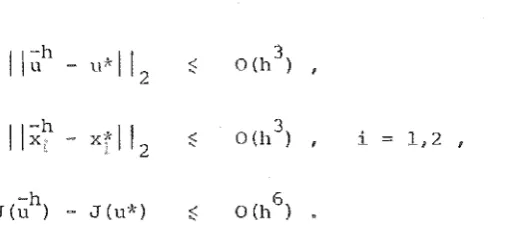
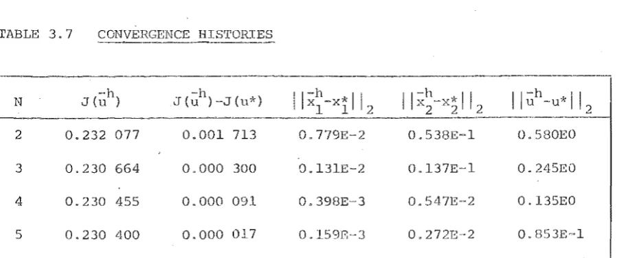
imations over spline spaces, explicit o:cder bounds are

derived. Computational results supporting these error

bounds are presented.

The State Parametrization Procedure.

The SP procedure for solving optimal control problems is

developed. The procedure is then specialised to the class

of control problems whose state equations can be expressed

in the phase variable fo:cm. Computational results employing

cubic splines are presented for two specific examples.

Error Bounds for the State Parametrization Procedure.

Convergence of the SP procedure is examined. Error bounds

for the SP approximations over spline approximation spaces

are es-tablished for a class of control problems.

The State Parametrization Procedure for Distributed Parffineter

Systems.

The SP procedure is extended to a wide class of distribllted

control problems. Con~utational results using multivariate

splines in conjunction with the SP procedure are presented.

The convergence of the procedure is also examined.

General Conclusions.

The contributions of this thesis are slmmlarised and directions

REFERENCES

R. Bellman: Dynamic Programming, Universit.y Press,

Princeton, N.J., (1957).

L. S. , V. G. Boltyanskii, R. V. Gamkrelidze and

E. F. Mishchenko: rrhe Mathematical of Optimal Processes,

Wiley, N.Y , (1962).

[3J R. E. Larson: State Increment Dynamic Programming, American

Elsevier, N.Y., (1968).

R. Bellman and R. Kalaba: Quasi1 and Nonlinear Boundary Value Problems, Elsevier Press, N.Y., (1965).

E. S. Lee: inearization and Invariant Imbedding, Academic

Press, N.Y., (1968).

P. B. Bailey and L. F. Shampine: On Methods for TPBVP, J. Math. Anal. and Appl., Vol.18 (1967) pp.45~58.

[7] A. P. Sage: Optimum Systems Control, Prentice-Hall, Englewood Cliffs "

N.J., (1968).

H. J. Kelley: Method of Gradients, in Techniques,

G. Leitman ed., Academic Press, (1962).

[9J L. S. Lasdon, S. K. rHtter and A. D. Waren: The Conjugate Gradient

Method for Control Problems, IEEE Trans. Automatic

Control, AC-12 (1967) pp.132-138.

R. Fletcher and C. Reeves: Function JVIinimization by Conjugate

[13J

[16J

D. Tabak and B. C. Kuo: Optimal Control by Mathematical Programming,

Prentice-Hall, Englewood Cliffs, N.J., (1971).

L. A. Zadeh and B. H. Whalen: On Control and Linear

Programming, IRE AC-7 (1962) pp.45-46.

S. Vajda: Ma'thematical Programming, Addison--Wesley, Reading,

Mass. (1961).

G. B. Dantzig: Linear Programming and Extensions, Princeton

University Press, Princeton, N.J., (1963).

P. Wolfe: The Simplex Method for Quadratic Programming, Econometrica,

Vol.27 (1959) pp.382-398.

G. Zoutendijk: Methods of Feasible Directions, Elsevier, Amsterdam,

(1960) •

J. B. Rosen: The Gradient Projection Method for Nonlinear Programming I: Linear Constraints, SI~i J. . Math., Vol.S (1960),

pp.181-217 .

J. B. Rosen: 'The Gradient Proj ection Method for Nonlinear Programming II~ Nonlinear Constraints, SI~l J. . Math., Vol.9 (1961)

pp.514-532.

C. W. Carroll: The Created Response Surface Technique for Optimizing

Nonlinear Restrained Systems, Op. Res., 9 (1961).

A. Fiacco and G. HcCormick: Nonlinear

Unconstrained Minimization Techniques, wi

Sequential

, N.Y. (1968).

[2

R. Hooke and T. A. Jeeves: Direct Search Solution of Numer::'cal and

Statistical Problems, Journal of the ACH, Vol.8 (1961), pp.212··

[22J

H. H. Rosenbrock: An AutomCltic Method for Finding the Greatest::

or Least Value of a Function, Computer J., Vol.3 (1960),

pp.175-184.

[23J M. J. D. Powell: An Efficient Method for Finding the Minimum of

a Function of Several Variables without Calculating Derivatives,

Computer J., Vol. 7 (1964) pp 147-151.

[24J

J. Kowalik and M. R. Osborne: Methods for Unconstrained Optimizat.ion·

Problems, Elsevier, N.Y., (1968).

[25J M. Hestenes and E. Stiefel: Method of Conjugate Gradients for

Solving Linear Systems, Report 1659, National Bureau of

Standards, (1952).

[26] R. K. Mehra and R. E. Davis: A Generalized Gradie:t:lt Nethod for Optimal Control Problems with Inequality Constraints and

Singular Arcs, IEEE Trans. Automatic Control, AC-l7 (1972)

pp.69-79.

[27J R. Fletcher and M. ,J. D. Powell: A Rapidly Convergent Descent Method for Minimization 1 Computer J. I Vol. 6, (1963).

[28J H. H. Rosenbrock and C. Storey: computational Techniques for

Chemical Engineers, Pergamon, London (1966).

[29J W. E. Bosarge, Jr. and O. G. Johnson: Direct Nethod Approximation to the State Regulator Problem Using a Ri tz-Trefftz SuJ:loptimal

Control, IEEE Trans. Automatic Control, AC~15 (1970)

pp.627-631.

1)

oJ

L. L. Lynn, E. S. Parkin and R. L. Zahradnik: Near-Optimal ;::ontro1 by ec Approximation, Ind. Chem Fund., Vol.9

[31J W. E. Bosarge, ,Jr., O. G. Johnson, R. S. McKnight and

v'l.

P. 'l'imlake:

The Ritz-Galerkin Procedure for Nonlinear Control Problems,

SIAM J. Numer. AnaL, VoL 10 (1973), pp.94-llL

[32] C. P. Neuman and A. Sen: Weighted Residual Methods in Optimal Control,

IEEE Trans. Automatic Control, AC-19 (1974) pp.67-69.

[3~

G. J. Lastman: Suboptimal Open Loop Control of Nonlinear Systems

Using Approximations for the Controls, Int. J. Con·trol, Vol.20

(1974), pp.289-303.

[34J W. E. Bosarge I Jr., and O. G. Johnson: Error Bounds of High Order

Accuracy for the State Regulator Problem via Piecewise Polynomial

Approximations, SIAM J. Control, Vol.9 (1971), pp.15-28.

[35J A. G. Butkovskii and A. Ya. Lerner: '1'he Optimal Control of Systems

wi th Distributed Parame"ters, Automation and Remote Control,

Vol.2l (1960) ~ pp.472-477.

A. G. Butkovskii: The Maximum Principle for Optimum Systems with

Distribut~ed Parameters, Automation and Remote Control, Vol.22

(1962), pp.1156-1169.

~

P. K. C. Wang: control of Distributed Parameter Systems, Advances

in Control Systems, Academic Press, N.Y. (1964).

[38J A. V. Balak.rishnan: Optimal Con tro 1 Prob lems in Banach

SIAM J. Control, Vol.3 (1965).

[39J J. L. Lions: Optimal Control of Systems Governed by Partial Differential Equations, Springer-Verlag, Berlin (1971).

[J~J J. H. Holliday and C." Sto:n:;y: Numerical Solution of Certain

Nonlinear Distributed Parameter Opt.imal Control Problelrs I

[4jj D. E. Cornick and A. N. Hichel: Numerical Optimization of

Distributed Parameter Systems by the Gradient

Method, IEEE Trans. Automatic Control, AC-17 (1972) pp.358-362.

A. P. and S. P. Chaudhuri: Gradient and Quasilinearization Techniques for Distribu'ted Parameter Systems,

Int. J. Control, VoL6 (1967) pp.81-98.

[43J C. P. Neuman and A. Sen: A Rapid Sub-Optimal Control Algorithm

for Dist:r:ibuted Parameter Regulator Int. J. Control,

Vol.16 (1972) pp.539-548.

[44J L. L. Lynn and R. L. Zahradnik: The Use of Orthogonal Polynomials

in the Near-Optimal Control of Distributed by Trajectory

, Int. J. Control, Vol.12 (1970), pp.1079-1087.

W. E. , Jr., O. G. Johnson and C. L. Smith: A Direct Method to the Linear Parabolic Problem over

Mul t i variate Spline Bases, SIAl"I J. Numer. AnaL, VoL 10 (1973)

pp.35-49.

[46J R. S. McKnight and W. E. Bosarge, Jr.: The Ri tz-Galerkin Procedure

fOT Parabolic Control Problems, SIAM J. Control, VoLll (1973)

pp.510-524.

[n]

G. Strang and G. J. Fix: An Analysis of the Finite Element Method,

Prentice-Hall, N.J. (1973).

A. E. Jr. and Y. C. Ho: Appli(~d Optimal Control, Blaisdell,

T. J. Walder and C. Numerical Solution of an Optimal

Temperature Problem, The Chemical Engineering J . , VoL 1 (1970) pp.120--128.

[so]

J. H. Ahlberg IE. N. Nilson and J. [ j . ~valsh: The Theory of Splines

and Their Applications, Academic Press, N.Y. (1967).

[511

H. G, Go1:tlieb: Rapid Convergence to Optimum Solutions using a

CHAPTER 2

'rEE CONTROL PARi"METRIZATION PROCEDURE

2.1 INTRODUCTION

The primary purpose of the present chap-ter is to revievl the control

parametrization (CP) procedure for solving optimal control problems with special emphasis on the use of spline functions

Suppose that we have an optimal control problem requiring the

minim-ization of a cost functional J (u) over 'the space of admissible controls U.

The CP procedure discretizes the problem by restricting the control variable to a subset C of U which is parametrized by m real variables.

m This involves

specifying the members of C ,to be of the form,

m

u(t) F(q,t) (2.1)

m

where F is a known function of the m-dimensional parameter vect~or qeE .

The function F specifies the form of the parametrization.

If only controls belonging to C are considered, then the cost m

func,tional reduces to a iU,l1ction of q, and we write,

J (u) J (q)

The original goal of minimizing J(u) over U is now replaced by that of

(2.2)

minimizing J(q)' over C .

m Assuming the existence of a solution, the new

problem of determining the optimal values of q l ' . · ' ,qm is generally a much

simpler task 'than t~he original problem which involves optimiza'tion in

'rhe case when F is a linear function of q is of particular

importance i equation (2.1) 1.:hentakes the form

m

u(t) L:

i=l

q.1jJ. (t) (2.3)

1 1

where ~J l ' . . . ,1jJ m are known functions of time called basis functions. In

this case C becomes an m-dimensional linear space over the scalar field E,

m

and we call C an approximation subspace of U. m

Sometimes the basis functions can be specially constructed to suit

the problem in hand (see [lJ,

[2J).

Otherwise standard families of functions may be used, some examples being the polynomials, trigonometric

functions, Legendre polynomials, Bessel functions and Hermite polynomials.

Extensive computational results using Chebyshev polynomials have been

reported by Lastman

[16].

Hicks and

[2]

presented computational results employing a control parametrization consisting of a bang-bang portion followed by a polynomial

curve. The parameters to be optimized in this case are (a) the switching

times for the bang··bang portion and (b) the coefficients for the polynomial

curve. The static optimization was performed using the direct search

technique of Rosenbrock. However/ this to be rather unsatisfactory,

as nominal controls tended to converge to different final controls,

even -though the final values of the cost were in close agreement with one

another. This difficulty appears to be due to the flatness of the cost

surface in the vicinity of the optimum, which causes direct search methods

.to be severely affected by truncation and round-off errors in compnting the

cost.

In view of this problem, Sirisena

[J]

suggested that the static

extended to problems involving constraints [4J.

In section 2.3 we review the basic CP procedure for the unconstrained optimal control problem. Extension of the procedure to problems with

terminal constraints is reviewed in section

2.4.

In sections 2.5 and 2.6 the transformation technique for converting problems involving control or state variable inequality constraints into unconstrained problems is reviewed. Throughout, the use of spline functions has been emphasised. The fundamentals of func·tions will now be reviewed.

2.2 REVIEW OF SPLINE

A function (or spline) is a polynomial which satisfies a strong smoothness condition. It is a natural generalisation of the polynomial, yet i t possesses certain features not shared by polynomials which make it attractive for the purposes of interpolation and approximation. For a comprehensive treatment of spline functions refer to the text by

Ahlberg, Nilson and Walsh

[5

J .

In this section \ve review some basic facts about spline functions. We shall begin with a couple of definit.ions.

Definition: Consider an interval ,bJ on the real line and a strictly increasing sequence of real numbers t ,tl, ... ,t , where

o N

a to < t l < ••• < tN b.

The set

P

=

{t ,tl, ... ,t } is said to be a partition of

o N ,bJ, and the

elements of P are called kno'cs (or nodes). The mesh size h of P is defined by

De Given a p _{{t ,tl, .•. ,t } of the interval}

o N

,b] ,

a function s(t) of a with knots t ,tl, ... ,t is a function

o N

defined on [a,b] having the following

(i) in each sub-interval (ti,t

i+l ), where i ~ O,l, ... ,N-l,

s(t) is a polynomial of a or less.

(ii) s(t) and its derivatives of order up to a-.l are continuous in

(alb)

It is clear from the above definition that a spline function of

a is a function in 1[a,b1 whose derivative of order a is piecewise

constant.

Given a partition P {t ,tl, .. o,t }, let us now consider the set

o N

of all splines of degree a over the partition P. It is easy to see that such a set is a linear space over the field of real numbers. NOw, each

spline s(t) in the space is continuously differentiable (a-I) times in

th

and the a derivative of s Ct) is a constant in each sub-interval

(t

i ,t;i+l) I i=O, I, ... ,N-I. Hence s(t) is parametrized by the initial

values of s(t) and its first (a-I) derivatives together with the value of

. th d " h u b ' 1 ( l·ts a erlvatlve over ea,c s -lnterva t. t

1

I i=O,l, . . . ,N-l.

Therefore, the dimension of this linear space is N+a, and henceforth i t

a+l . a+l

shall be denoted by S (t " " / t ), SN' or

o N

basis

Bases

It follows from the theory of linear spaces that there exists a

a+l

containing N+a elements for the spline space

S

(t , ... , t ).

a N

1'4oreover, this basis is not unique. To construct one such basis, we note

a+l

that every s(t) E

s

(t " " I t ) can be

o

N

in the form

where p (t) is a polynomial of degree c( or less, and (t- ) 0. is the

0. +

truncated power function defined as follows:

r

(t_t,)o.

,

_{if t ?; t.}

t

1 1

(t-t, )0. 1 +

0 if t ~ t.

1

(2.6)

0. 0. 0.

Therefore the set {l/t, ... , t , (t-t~)+, ... , (t-t

N_1)+} is a basis for

1

(t p • • , t ) .

o N

The B-splines of Schoenberg

[6J

provide another possible spline

basis. In spline interpolation problems, the use of B-splines gives rise

to better numerical stability than the use of bases constructed with

tn.mcated power functions (see

[91).

A feature of the B-spline is that i t has fini·te supporti that is l i t is non-zero only on a finite region.

In fact, i t was shown by Curry and Schoenberg

[7J

that the B-splines are

of minimal support; that is, no other basis functions can be found which

have smaller support regions than those of the B-splines. Another property

of the B-spline is that i t is strictly positive within its support region

which'is restricted to 0.+1 adjacent intervals.

Let us consider now the bi-infinite partition {t.}~ of the real

J. 1==-<0

line. The B--spline

IP.

(t) of degree 0, which is non-zero over the in-terval

1

(ti,ti+o.+l) is given by the formula,

lji,(t) :=

1 (t, 1+0.+ I-t, ) 1

i+o.+l

l:

j==l

i+o.+l {(t,-t)o./ II

J + _m=i

mfj

(t ,-t )}. (2.7)

J m

·The above definition provides the normalized form of the B-splinej in other

words,

1 (2.8)

In the case of a uniform partition, the of order ex are

merely translates of one another along the real line. To illustrate this

point, suppose that the knots in the partition are given by t. = jh for all J

j, where h is the constant mesh size of the partition. Then i t

can be shown that,

~J.(t) == ljJ.('t-t . . ).

1 J 1 - J

(2.9)'

Furthermore, a change in the mesh size of the uniform partition simply

means a re-scaling of the independent variable in the formula for s.

Consider the partition Z == {i}~ whose nodes are the integers, and let

1=-00

ljJ(t) be the of order ex which is non-zero over the interval [i,

{t.}~ is ano·ther uniform partition, wher'e t. = ih,

1 1=-00 1

and let ¢(t) be the B-spline of order ex which is non-zero over the interval

<P (t)

The functions IjJ and <P are then related by the formula

IjJ

(~

- j+i)

h (2.10)

The B~spline ljJ(t) starts from zero at t if monotonically increases

t i l l i t reaches its maximum at the poin1: t i + (a+l)/2, then monotonically

decreases t i l l i t returns to zero at t

=

i -I- a

+

1. Horeover, IjJ is

symmetrical about its point of maximum. Explicit formulas for typical

B-splines of orders 1, 2 and 3 over the partition Z are (i) linear spline

r

1

+

t, ~) (t) :=

'\ 1 t,

l,

a

(ii) parabolic spline

l-~J (t)

l(

)2

2 I t t ,

]

--2 + t

2 ' ' 0 2t

+

0,

2

t I

1 2

~t

2' f

t

Eta]

tE:

[o,lJ

elsewhere

t £:

,0]

t £ [

O,JJ

t E [ 1,

~I

(iii)

cubic spline

(1

) 3

6

2+t

,

t E:

2 2 1 3

3

t

2

t ,

t E:

[--1,0 ]

lj!

(t)

:::: 2

t

2

1

3 -1-

2

t E:

[0,1

J

1 3

I

6(2~t) I t £

[1,2 ]

L

a

elsewhere

2.3 PROBLEMS WITHOUT

In this section we review the CP procedure for the unconstrained

Bolza problem.

Although spline approximation spaces are employed here,

the method to be described can be generalised to the case of a general

parametrization with obvious modifications.

For clarity of presen·ta·tion,

only single-input systems will be considered; the generalisation to

multivariable systems is straightforl.vard.

Problem

Consider the dyn<Jmical system described by

x(t)

f(x(t), u(t),

t ) ,

and the cost functional

x (0) x

o

J(u)

==

O[X(T) ,TJ

+

f~

¢(x(t), u(t), t) c1t,

where x(t) is an n-dimensional s·tate vector and u(t) is

a

scalar-valued

control variable belonging to the set of admissible controls

U.

The

(2.11)

(2.12)

optimal control problem is to find the admissible control ul< that minimizes

the cost fW1ctional: '

Method

Firstly, a suitable partition of the time interval [O,,z] is chosen.

For convenience, we shall assume that the partition is uniform:

o

==

T

where N is the number of sections into which

,T]

is divided by the parti'tion, and t.

J jh (O:Sj:SN), where h = TIN is the uniform mesh size.

h

An

arbitrary spline function 1.1 of order a over the partition (2.13)

may be expressed in the form

h

\1 (t) ::::

N+a

l:

i==l

q.lj!. (t) I

1 1 (2.14 )

a+l

where {lj!l ,lj!2

,···,lj!N+a}

is a basis for the spline space Sh . In general,

a+

U will be the space of piecewise continuous controls, so S h U fo.r

non-negative integer

a.

-h

a+l

TheCP procedure involves finding the control u € Sh which

minimizes the cost functional:

. a+l . h

It is clear that 51.nce 8

h 1S a subset of U, we must ave that

J(u*) :S J(rih) , so in general;h will only be sub-optimal.

(2.15)

For a given basis {lj!l ,lj!2 , ... ,lj! }, the control u is parametrized

N+a

Hence the functional J(u) may be

considered an o;rdinary function of these parameters, and we write

-J(u) - J(Ql,Q2, ... ,QN+a)' (2. 16)

It was

recorrul1~nded

by Sirisena

[3J

that the optimization of J be

performed using a 'Jradient search method, for insta.nce the

requires the evaluation of t:he yradient of J with respect to each parameter

q. . 'l'hese gradients may be computed as described below.

1

The Hamilton H is defined in the usual manner,

H(x(t) ,u(t) ,;\(t) ,t) :: ~(x(t) ,u(t) ,t)

+

<;\(t) ,f(x(t) ,u(t) , t » .

The co-state equations are given by

dH

dX '

de [.:.:(T) ,T]

dx(T)

and by standard vari ai.:ional arguments, i t can be shown that

Remarks

3J 3q.

1

dH

-;:;:-:- 1J.i. (t)dt

aU 1 i 1,2 , ••. , N+a

(i) As the number of sections N is increased, we do not necessarily

(2.17)

(2.18)

(2.19)

have a monotonic decrease in the minimum cost

J(~h),

unless the partition

is successively refined.

(ii) The internal knots t l , t , . . . , t of the partition may be assumed

2 N-l

to be variable, and treated as additional parameters to be optimized.

Expressions for the gradients of J with respect to these knots have been

derived in

[3J.

It is clear that whereas the control is a linear function

of the parameters q ,q , . . . ,q , i t is a nonlinear function of the variable

1 2 N+a knots t l , t , ... , t

2 N+a If the optimal control profile is smooth, there is probably not much to be gained from using variable knots. However, i f there

are discontinuities in the optimal control profile, i t would almost cert:ainly

be profitable to optimize the internal knot locations as well.

(iii) 'l'he parametrization introduced by Sirisena in

[3J

implicitly employs

a basis which is closely related to the truncated power functions; the

basis functions are 6f the form

i .=:: l,2, .... ,a

2.4 PEOBLEMS WI'l'H TERMINl\L CONSTRAINTS

In this section we briefly review the CP procedure for problems in which the st,ate vector is constrained at the final time. The procedun~

to be described here is due to Sirisena and Tan [4J.

The problem statement of section 2.3 is assumed, with the addition of the following terminal constraint:

1) [X(T) ,T]

=

0, (2.20)

where 1) is an t-dimensional vector.

Method of Approach

As in the procedure for the unconstrained problem, the first step

is to select a suitable partition. The control is then parametrized as a

spline function as in equation (2.14).

The terminal constraint (2.20) is treated as ~ equality constraints on the parameters ql"'" ~+a . The optimization subject to equality cons'traints can be handled using numerical techniques like the gradient

projection algori,thm of Eosen. Further details concerning the implementation

of the CP procedure may be found in [4J.

Eemarks

Given a particular problem, and assuming that N and a are fixed,

. . a+l h h . 1 .

must there always eX1st a control ],n Sh suc that t. e term1na constral.nt

1)

[x

(T) ,T]

o

is satisfied? Intuitively, we feel that, provided N and a

are sufficiently large, such a control should indeed exist.

We can show this to be true for a constant linear system. Suppose

that the following system

x ::::

Ax + bu (2.21)

n-dimensional vector" (The dependence, of x and u on t have not been

explicit,ly above for the sake of notational convenience).

'Ehen the augmented syst,em

(2.21a)

wi th u _(1.+ 1 as the new control variable can be shown to be cont.rollable by

applying the usual controllability criterion, (see

[11J).

Suppose now that we require u I to be piecewise constant. This cH

is equivalent to the introduction of sampling to the system (2.21a). The

effect of sampling on the controllability of a continuous linear system

has been investigated by Kalman, Ho and Narendra [lOJ for the case of

constant sampling period. It was found tha·t, provided the sampling

frequency is sufficiently large, there should be no loss of controllability.

Hence the (2.21) is controllable using only elements of Sh 0.+1

provided that the mesh size h is small.

Notation

Henceforth we shall simplify our notations by omitting the argument

list after each function whenever i t is convenient to do so without causing

confusion.

2.5 PROBLEMS WITH CON'l'ROL CONSTRlUNTS

Optimal control problems occurring in practice often involve

inequality constraints on the state and control variables. These constraint-:s

C(x,u,t) ~

o.

(2.22)

When the function C is independent of x, the constraint is then called a control constraint:

C (u,t) ~

o.

By far the most important class of control constraints is that of saturation-type constraints of the form

c(t) ::. u(t) ;;: d(t) (2.23)

In this section we demonstrate that ·the CP procedure is applicable to problems involving saturation-type constraints through the use of suitable transformations of variables. Problems involving state constraints are considered in sec·tion 2.6.

Problem Statement

~'le consider here the problem of minimizing the cost functional

for the n-dimensional system

x

f(x,u,t) , x(o)

x

o

subject to the con-tl:ol constraint (2.23). For the sake of clarity we shall assume C and u to be scalar-valued functions.

Method of

The transformation technique we use here involves 'defining the control variable u in terms of a new variable

v

by means of a suitable

(2.24)

(2.25)

'Elms, for the const_raint (2.23) we define the new variable \) by.

u (t)

6(\),t) ,

(2.26)

where

e

is any function that satisfies the condition

c(t) ~

e

(\),t) ::: d(t) (2.27)

for all possible values of

v.

The CP then proceeds with the parametriza-tion of the new control variable

\)(t) F(q,t) (2.28)

where q is the m-dimensional parameter vector.

We nOVl need to derive the gradient of the cost J(q) with respect to q. Using standard variational

aH

a\)

av

dt I

where H is the Hamiltonian defined in the usual way, H :: ~

+

<A,f> I

and A- is the co-state vector given by

ClH

dX I

I we can show that

Finally, using. (2.26) and (2.28), 'ehe expression (2.29) may be written

dB dU

of Transforma-tion

de

dV

dF

dq dt.

(2.29)

(2.30)

(2.31)

(2.32)

We now look at tvlO possible forms of the -transformation

e.

The first example is one which is well known in the context of mathematical programming (see [12J):

e

(v,t)

+

However, the computation of transcendental functions is quite expensive,

and a computationally simpler aH:ernative is the f0110win(j transformation:

d (t) , if vet) > d(t)

6(v,t)

v

(t) , if c(t)

:s

vet) :S d(t) (2.34)

c (t) , if vet) < c(t)

The main draw-back of the above "clipping" transformation is that

converg-ence to the solution is not always obtained. For instance, i f the

nominal control lies completely outside 'the feasible region, the CP procedure employing the transformation (2.34) breaks down. Nevertheless, in those

instances when i t does work, i t appears to work well. Highly satisfactory

computational results using the "clipping" transformation in conjunction

with the CP have been reported by Sirisena and Tan

[4J.

Numerical Example

The CP described above was used to solve the following Rayleigh problem which was taken from [13J.

For the described by

(0) -5

find the control u* that minimizes

J

J

o

2.S(

xl 2

+

u 2) dt

Subject to the control magnitude constraint

I

u (t)

I

:s

1 for all t E

LO

I 2 .

The transformation (2. 33) ~'las to reduce the above

to an c. unconstrained problem in the new control variable \! given

u :;; sin \) .

The variable \) was parametrized as a pal':abolic spline over a uniform

of ,2. with N sections. 'l'he problem was solved for N=2 and N=4; and for each N used, two nominal controls were employed, viz. \):::0

It was found that the control converged to the same value

afte):: fl':om the two different nominal controls. The

control for N==2 and N=4 are summarised in Table 2.1. 'I'he minimum

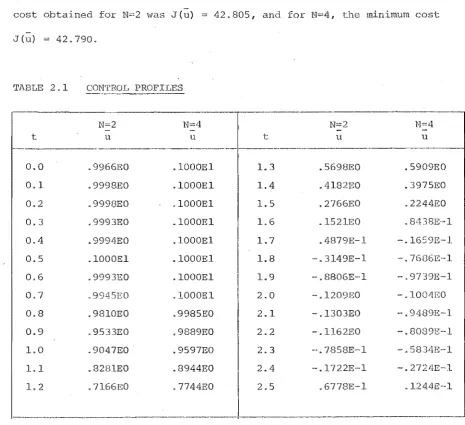
cost obtained for N=2 was J (u) = 42.805, and for N=4, the minimum cos·t

J(u) == 42.790.

TABLE 2.1 CONTROL PROFILES

-~"'~""

N=2 N==4 N==2

-

_-

-t u u t u u

---~ .. -~

0.0 .9966EO .1000El 1.3 .5698EO .5909EO

0.1 .9998EO .1000El 1.4 .4182EO • 3975EO

0.2 .9998EO .1000El 1.5 .2766EO .2244EO

0.3 .9993EO .1000El 1.6 .1521EO .8438K-l

0.4 . 999tJEO .1000El 1.7 .4879E-l -.1659E-I

0.5 .1000El .1000El 1.8 -.3149E-l .76B6E--l

0.6 .9993EO .1000El 1.9 -.8806E-·1 -.9739E-l

0.7 .9945EO .1000El 2.0 -.1209EO -.1004EO

0.8 .9810EO .9985EO 2.1 -.1303EO -.9489E-l

0.9 .9533EO . 9889EO 2.2 -.1l62EO -.8089E-l

1.0 .9047EO • 9597EO 2.3 '".7858E-l .5834E-l

1.1 .8281EO . 8944EO 2.4 -.1722E-l -.2724E-l

1.2 .7166EO . 7744EO 2.5 .6778E-l . 1244E .. l

[image:40.555.55.521.241.666.2]

2.6 PROBLEr.1S WITH S'I'Nl'E

We considered the use of appropriate tY'ansformai:ion in section 2.5

to handle control constraints. This approach is extended here to problems

involving state constraints of the form (2.22) in which the constraint

function C contains the state x explicitly.

The system equation (2.25) and the cost functional (2.24) are

assumed here. We begin defining a new variable zthrough the

trans-formation

c(x,u,t) :::: 8(z,·t) (2.35)

where 8(z,t) is a negative function. We assume here ,that C is linear in

x and u. This assumption ensures that the form of the constraint function

C does not implicitly impose constraints on z. And i t was for the same

reason that we only considered saturation-type control constraints in the

previous section. Fortunately, the linearity of C is not a restrictive condition, as most constraints appearing in control problems are formulated

as linear constraints.

Having specified the transformation (2.35), we can then obtain the

transformed (unconstrained) problem following the procedure described in

[14]

by Jacobson and Lele. In that article, the authors suggested using

the particular transformation

8(z,t) (2.36)

Nevertheless, any negative function 0 may be used, and the procedure

. described in.

[)4]

regarding the conversion of the original problem to the new unconstrained problem to the general case with obvious

Basically, there are two cases to consider. If C con"tains u

explicitly, equation (2.35) can be solved for 1.1 in terms of

x

and

z,

and 1.1

can be eliminated from the original optimal control problem. The result

is an unconstrained problem in the new control variable z. If C does

not contain u explicitly, then the equation (2.35) is differentiat.ed with "to t unt.il 1.1 appears. that the constraint (2.35) is

of order Pi -that is, u appears for the first time in dPC/dtP • Then the original problem converts into an unconstrained problem of increased

dimension , with the new control variable dPz/dt

P .

Numerical

The method described above was applied to two sample problems.

The transformation of Jacobson and Lele were employed to reduce each problem

to an unconstrained one. And in each case the new control variable was

parametrized as a linear

Example L

rvIinimize J

for the

x(o) == 0 subject to the first-order constraint

x(t) ~ sin(nt)

+

a •

where a _ n/3/12 - .5 == -.046550 (to 5 significant figures).

This problem has been taken from

[lSJ.

and has the exact solution

J

6a

+

3 I

o

:s

t

..

< 1/6 1.1* (t) ncos(nc) r 1/6

_:::

t:::

1/2

The minimum cost for the problem is

J*

= 1.0992

(to

5

significant figures)

Employing<the transformation (2.36), we have

x (t)

sin(l1t)

a ==

"2

1 z 2 (t).

By differentiating the above equation and making use of the state equation,

we obtain

U

zZl

+

l1C08(l1t) ,

where zl

Z.

From the above defining equation for z, we find that

z(O)

1~':2a

(we could have chosen the initial condition

z (0) :::: - 1=2a ,

bu·t it

does not matter which one is used).

The transformed problem is then:

minimize

J

for the system

1

2

x

=

zZl

+

l1COS(l1t)

x(o)

o

0)

=

Because the state x is not present in the performance index, the corresponding

s-tate equation is actually now redundant.

Our new control variable is z

,and we parametrized i-t as a limc:ar

1

spline over a uni form partition of

[0,

IJ wi th N sections.

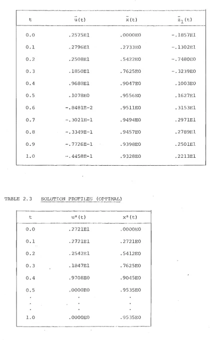
A solution was

obtained for N=5, and the minimum cost obtained was

1.1014,

The approximate solution obtained is summarised in '['able 2.2, whi Ie the

TABLE 2.2

t u(t) x (t)

0.0 .2575El .OOOOEO

0,1 .2796El .2733EO

0.2 .2508El .5422EO

0.3 .1850El .7625EO

0.4 . 9688El .9047EO

0.5 .1078EO .9556EO

0.6 -.8481E-2 .95l1EO

0.7 -.3021E-l . 9494EO

0.8 -.3349E-l .9457EO

0.9 -.7726E-l .9398EO

1.0 "".4458E-l .9328EO

TABLE 2.3 PROFILES

t u*(t) x,~ (t)

0.0 • 2721El .OOOOEO

0.1 .2721El . 2721EO

0.2 .2542El .54l2EO

0.3 .1847El .7625EO

0.4 .9708EO .9045EO

0.5 .OOOOEO .9535EO

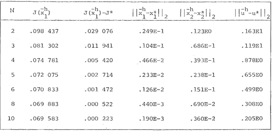
[image:44.555.57.489.80.762.2]

2

. . . J -_ fl (x2

+

2 5 2) d

Mln1mlze 0 1 x

2

+

.00 u t

for the second-order system

:::::

+

_u,

ect to the first-order constraint (t) S(t-.5) 2 +.5 ~ O.

This problem has been taken from [14J. Application of -the ·trans-formation (2.36) gives rise to the following unconstrained problem

-ZZI

+

16t - 8 --I

z z (0)

=

-15

J

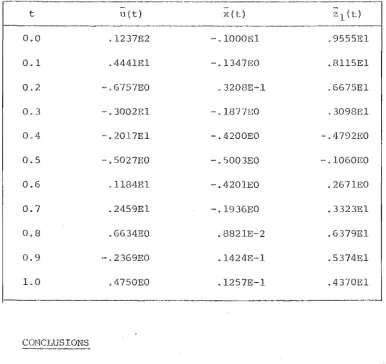
The new control variable zl ,vas parametrized as a linear over a uniform of [O/IJ containing N sec·tions. The problem was solved for N=5, and the results are summarised in Table 2.4. 'l'he minimum cost obtained was

0.17177.

The above was solved by Lastman [16J using Chebyshev polynomials in conjunction with the CP procedure. He obtained the minimum cost 0.17401

TABLE 2.4 SOLu'rION PROFILES

t

0.0

0.1

0.2

0.3

0.4

0.5

0.6

0.7

0.8

0.9

1.0

2.7 CONCLUSIONS

In this

optimal control

u(t) x(t) ~~l (t)

.1237E2 -.lOOOEI ,95

. 4441El ~.1347EO • B115E

-.6757EO . 320SE-I

.3002El - .1877EO

-.2017EI -.4200EO .4

-.5027EO -.5003EO

. 1184El -.420lEO .267

.2459El -.l936EO .332

.6634EO .882IE-2 .6

. 2369EO .l424E-l .5

. 4750EO .l257E-l .4

we have reviewed the CP procedure for

vii th fixed final time. The basic ,vas first described for the unconstrained problem. It was then seen thal the

procedure could be to problems involving terminal constraints

because such constraints can be treated as equality constraints on the

parameters. It was also 8ho;"n that problems Itlith control or state variable

inequality constraints could be handled through the use of

transformations of variables to co~vert these constrained

unconstrained ones.

We have also reviewed some basic material on

t:he use of splines in the CP procedm..? has been

into

functions, and

Finally,

some :cesulLs of employing splines in conjunct.:lon with the CP

[image:46.555.87.474.100.464.2]

REFERENCES

[1] T. J. Walder and C. Storey: Numerical Solution of an Optimal

Temperature Problem, The Chemical Engineering J., Vol.l (1970) pp.120-l28.

G. A. Hicks and W. H. Approximation Methods for Optimal

Control Synthesis, Can. J. Chern. Eng., Vol.49 (1971) pp.522-52a

[3] H. R. Sirisena: Computation of Optimal Controls Using a Piecewise

Polynomial Parametrization, IEEE Trans. Automatic Control,

AC-18 (1973) pp.409-4ll.

[4J H. R. Sirisena and K. S. Tan: Computation of Constrained Optimal

Controls Using Parametrization Techniques, IEEE Trans. Automatic

Control, AC-19 (1974) pp.43l-433.

[5J J. H. Ahlberg, E. N. Nilson and J. L. Walsh: ']~he Theory of Splines

and Their Applications, Academic Press, N.Y. (1967).

[6J I. J. Schoenberg: Contributions to the Problem of Approximation of Equidistant Data by Analytic Functions, Quart. • Ma·th. 1

Vol.4 (1946), Pt A, pp.45-99i Pt B, pp.112-141.

[7J H. B. Curry and 1. J. Schoenberg: On Polya Frequency Functions. IV., J. Analyse Math., Vol.17 (1966) pp.71-107.

[aJ R. Fletcher and M. J. D. Powell: A Rapidly Convergent Descent

Hethod for r-1inimization, Computer J., VoL6 (1963) pp.J.63~·168.

[9 J T. N. E. Greville: Introduction to Spline Functions, in Theory

and Applications of Funct.ions, ed. 'r.N.E. GreviJle,