Blind Equalization for Tomlinson Harashima Precoded Systems

(1)

Blind Equalization for

Tomlinson-Harashima Precoded

Systems

Rubyet Adnan

A thesis submitted in partial fulfilment of the requirements for the degree of

Master of Engineering in

Electrical and Electronic Engineering at the

University of Canterbury, Christchurch, New Zealand.

(2)

(3)

ABSTRACT

At a communications receiver the observed signal is a corrupted version of the

transmit-ted signal. This distortion in the received signal is due to the physical characteristics

of the channel, including multipath propagation, the non-idealities of copper wires and

impulse noise. Equalization is a process to combat these distortions in order to recover

the original transmitted signal. Roughly stated, the equalizer tries to implement the

in-verse transfer function of the channel while taking into account the channel noise. The

equalizer parameters can be tuned to this inverse transfer function using an adaptive

algorithm. In many cases, the algorithm uses a training sequence to drive the

equal-izer parameters to the optimum solution. But, for time-varying channels or multiuser

channels the use of a training sequence is inefficient in terms of bandwidth, as

band-width is wasted due to the periodic re-transmission of the training sequence. A blind

equalization algorithm is a practical method to eliminate this training sequence.

An equalizer adapted using a blind algorithm is a key component of a bandwidth

efficient receiver for broadcast and point-to-multipoint communications. The initial

convergence performance of a blind adaptive equalizer depends on the higher-order

statistics of the transmitted signal. In modern digital systems, Tomlinson-Harashima

precoding (THP) is often used for signal shaping and to mitigate the error propagation

problem of a decision feedback equalizer (DFE). The concept of THP comes from

pre-equalization. In fact, it is a nonlinear form of pre-equalization, which bounds the

higher-order statistics of the transmitted signal. But, THP and blind equalization are

often viewed as incompatible equalization techniques.

In this research, we give multiple scenarios where blind equalization of a

THP-encoded signal might arise. With this motivation we set out to answer the question,

(4)

iv ABSTRACT

combination of a Tomlinson-Harashima precoder on the transmitter side and a blind

equalizer on the receiver side. By bounding the kurtosis of the THP-encoded signal, we

show that THP actually aids the initial convergence of blind equalization. We find that,

as the symbol constellation size increases, the THP-encoded signal kurtosis approaches

that of a uniform distribution, not a Gaussian.

We investigate the compatibility of blind equalization with THP-encoded signals

for both SISO and MIMO systems. In a SISO system, conventional blind algorithms

can be used to counter the distortions introduced in the received signal. However, in

a MIMO system with multiple users, the other users act as interferers on the desired

user’s signal. Hence, modified blind algorithms need to be applied to mitigate these

interferers. For both SISO and MIMO systems, we show that the THP encoder ensures

that the signal distribution approaches a non-Gaussian distribution. Using Monte Carlo

simulations, we study the effects of Tomlinson-Harashima precoding on the performance

of Bussgang-type blind algorithms and verify our theoretical analysis.

The major contributions of this thesis are:

• A demonstration that a blind equalizer can successfully acquire a THP-encoded

signal for both SISO and MIMO systems. We show that THP actually aids blind

equalization, as it ensures that the transmitted signal is non-Gaussian.

• An analytical quantification of the effects of THP on the transmitted signal

sta-tistics. We derive a novel bound on the kurtosis of the THP-encoded signal.

• An extension of the results from a single-user SISO scenario to multiple users and

a MIMO scenario. We demonstrate that our bound and simulated results hold

for these more general cases.

Through our work, we have opened the way for a novel application of training

sequence-less equalization: to acquire and equalize THP-encoded signals. Using our

proposed system, periodic training sequences for a broadcast or point-to-multipoint

system can be avoided, improving the bandwidth efficiency of the transceiver.

Fu-ture modem designs with THP encoding can make use of our advances for bandwidth

(5)

ACKNOWLEDGEMENTS

I would sincerely like to thank all those people who played a part in the completion of

this thesis. Special thanks to my supervisor, Dr. Lee M. Garth, for his guidance, help

and consistent encouragement.

Special thanks to my fellow postgraduate colleagues in the Communications

Re-search Group. I would like to thank you all for the times we spent together, sharing

knowledge in all of the meetings. You have made my postgraduate life more colorful

and precious.

I would also like to thank my parents for their love and consistent support in the

completion of this project and their encouragement of my pursuit of a higher degree

and achievements. Lastly, thank you Allah for your mercy, love and grace, being with

(6)

(7)

LIST OF FIGURES

1.1 Proposed blind equalization model for THP system 3

2.1 General model of a communication system 9

2.2 Decision Feedback Equalizer 11

2.3 Pre-equalization at the transmitter side 13

2.4 Block diagram of MIMO channel model 14

2.5 Decision Feedback Equalizer for a 2 _×3 system 17

2.6 SISO Tomlinson-Harashima Precoder 18

2.7 Output vs. input for the modulo adder 18

2.8 MIMO Tomlinson-Harashima Precoder 19

2.9 Graphical representation of CMA from [1] 21

2.10 Graphical representation of MMA from [1] 21

2.11 Graphical representation of RCA from [1] 22

2.12 MIMO system with linear equalizer 23

3.1 Training sequence mode for DFE 32

3.2 Use of feedback filter of DFE in precoder 32

3.3 Training sequence mode for MIMO DFE 33

3.4 Use of feedback filter of MIMO DFE in precoder 34

3.5 MMSE for different values for zero of the channel and propagation delay 37

3.6 Channel impulse response from [2] 38

3.7 MSE during training sequence 38

3.8 Comparison of DFE tap weight magnitudes 39

(10)

x LIST OF FIGURES

3.10 THP model for single-zero channel 41

3.11 Linear and nonlinear regions of the THP 42

3.12 Prefiltered signal kurtosis for 4-QAM over single-zero channel (a)

with-out and (b) with modulo operator 42

3.13 Prefiltered signal kurtosis for 16-QAM over single-zero channel (a)

with-out and (b) with modulo operator 43

3.14 2_×2 MIMO THP system 44

3.15 Prefiltered signal kurtosis for 4-QAM in u1(k) stream over single-zero

MIMO channel (a) without and (b) with modulo operator betweenu1(k)

and v1(k) 45

3.16 Prefiltered signal kurtosis for 16-QAM inu1(k) stream over single-zero

MIMO channel (a) without and (b) with modulo operator betweenu1(k)

and v1(k) 45

3.17 Sawtooth input-output function of the modulo adder 46

3.18 4-QAM (a) data source and (b) channel output constellations 51

3.19 Histograms of prefilter outputs for 4-QAM (a) without and (b) with

modulo addition 52

3.20 Histograms of prefilter outputs for 64-QAM (a) without and (b) with

modulo addition 53

4.1 Magnitude frequency response of 300 m of 0.4 mm distribution cable 56

4.2 Impulse response of 300 m of 0.4 mm distribution cable 56

4.3 Magnitude frequency response of composite VDSL channel 57

4.4 MSE Trajectory of DFE for VDSL Channel 58

4.5 Residual error for SISO system 59

4.6 Single-input multiple-output communications system 60

4.7 Adding a new user to a SISO system 60

4.8 Frequency responses of two different bandpass channels 61

4.9 Residual error for receiver of user 2 62

4.10 Equalizer output for receiver of user 2 62

(11)

LIST OF FIGURES xi

4.12 Equalizer output of user 2’s receiver for null channel 63

4.13 Residual error of user 2’s receiver for null channel 64

4.14 Equalizer output constellations in training mode for first receiver 65

4.15 Equalizer output constellations in training mode for second receiver 66

4.16 MSE during training for first receiver 66

4.17 MSE during training for second receiver 67

4.18 Equalizer output constellations for first receiver 68

4.19 Equalizer output constellations for second receiver 68

4.20 Receiver modulo output constellations for first receiver 69

4.21 Receiver modulo output constellations for second receiver 69

4.22 Residual error for first receiver 70

(12)

(13)

LIST OF TABLES

3.1 Kurtosis for M-ary ASK 48

3.2 Kurtosis for M-ary QAM 50

(14)

(15)

ABBREVIATIONS AND ACRONYMS

ADSL Asymmetric Digital Subscriber Line

ASK Amplitude Shift Keying

CMA Constant Modulus Algorithm

CSI Channel State Information

DFE Decision Feedback Equalizer

HDSL High Bit-Rate Digital Subscriber Line

i.s.i. Intersymbol Interference

i.u.i. Interuser Interference

LMS Least Mean Square

MIMO Multi-Input Multi-Output

MMA Multi Modulus Algorithm

MSE Mean Squared Error

MMSE Minimum Mean Squared Error

QAM Quadrature Amplitude Modulation

RCA Reduced Constellation Algorithm

SIMO Single-Input Multiple-Output

(16)

xvi ABBREVIATIONS AND ACRONYMS

SNR Signal-to-Noise Ratio

THP Tomlinson-Harashima Precoding

VDSL Very High Bit-Rate Digital Subscriber Line

(17)

Chapter 1

INTRODUCTION

1.1 BANDWIDTH-EFFICIENT COMMUNICATION SYSTEMS

Bandwidth is one of the precious commodities in modern high-speed communication

systems. With widespread broadband adoption the demand for bandwidth is constantly

increasing. The greater the bandwidth, the greater the scope is for achieving high speed

communications. From a commercial point of view, transmission power and speed are

the performance measures for any communication system. Example high speed wireline

communications systems are Asymmetric Digital Subscriber Lines (ADSL) and Very

High-Bit Rate Digital Subscriber Lines (VDSL) [4]. But, with a training sequence

overhead these connections do not exploit their full potential bandwidth. Each time a

user is connected to the receiver a training sequence has to be sent. To improve the

bandwidth efficiency of the system, this training sequence should be removed.

In recent times the use of multiple antennas at both sides of a communication

sys-tem has been widely investigated [5]. These so-called multiple-input multiple-output

(MIMO) systems can increase the channel capacity and overall transmission rate over

conventional single-input single-output (SISO) systems. Example MIMO systems

in-clude spatial division multiple access (SDMA) systems in wireless communications and

vector coded systems in VDSL wireline communications [6]. But, with the increase of

system capacity in MIMO communication systems comes more co-channel interference.

To combat this interference, the receiver needs to employ MIMO equalizers. At the cost

of bandwidth efficiency, a training sequence-based adaptive equalizer can again

sepa-rate and recover the multiple signals at the receiver. Again, the removal of training

(18)

2 CHAPTER 1 INTRODUCTION

1.2 ADAPTIVE EQUALIZATION

An adaptive equalizer is a crucial receiver component for a bandwidth-efficient

com-munication system. Because of its adaptive nature, it can track the changing channel

conditions and then reduce the distorting effects introduced by the channel. In a SISO

system, sources of distortion include the lowpass filtering by the channel and additive

channel noise. In a MIMO system, another source of distortion is interuser interference

(i.u.i.) due to the other users sharing the channel. SISO or MIMO adaptive equalizers

try to mitigate these effects and recover the original transmitted data within a certain

margin of error.

Conventional trained equalizers require exact knowledge of a portion of the

trans-mitted signal at the receiver. They compare the received data with the training

se-quence, adapting the equalizer taps to minimize a cost function such as the mean

squared error (MSE) [7]. But, for bandwidth-efficient communication systems,

par-ticularly broadcast or point-to-multipoint systems, bandwidth is wasted due to the

requirement of repeated transmissions of the training sequence. Blind equalizers, on

the other hand, are able to start up without a training sequence. Instead of using a

training sequence, blind algorithms depend on the higher-order statistics of the

trans-mitted signal.

A widely-used family of blind algorithms is based on the Bussgang algorithm, with

a relatively simple cost function which is directly related to the kurtosis of the

trans-mitted signal [8]. The effect of the source distribution on the convergence of Bussgang

equalizers has been investigated in [1], [9] – [12]. It has been found that the

conver-gence behavior is consistently good for platykurtic or sub-Gaussian sources [11]. Also,

the initial condition for successful convergence of blind equalizers has been found to be

dependent on the excess kurtosis of the combined channel-equalizer response [13], [14].

Thus, the distribution of the transmitted signal, characterized by the kurtosis, plays a

key role in the performance of Bussgang equalizers. As we will show, by bounding the

transmitted signal kurtosis, we can ascertain the potential performance of

Bussgang-type algorithms.

(19)

1.3 THE BLIND-THP SCENARIO 3

the training sequence, there are also alternative equalizer structures such as the DFE,

which can be used to get rid of the distortions in the received signal. The DFE has a

feedforward equalizer, a feedback equalizer and a threshold device. The presence of the

two equalizers in the DFE enables it to outperform a conventional linear equalizer in

terms of reduced MSE. But, because of its feedback structure, an incorrect decision by

the threshold device is fed back, leading to error propagation. When a reverse channel

is available, this error propagation can be eliminated by placing the feedback equalizer

in the transmitter.

Tomlinson-Harashima Precoding (THP) [15], [16] is a well known method to

elim-inate error propagation in a DFE. It has been adopted in a wide variety of modern

communication systems with reliable feedback channels. In this thesis we study the

effect of THP on the source distribution and blind equalization performance. We show

that THP bounds the higher-order statistics of the transmitted signal.

1.3 THE BLIND-THP SCENARIO

We now consider the combination of blind equalization and THP. Our goal is to study

the performance of blind equalization algorithms for Tomlinson-Harashima Precoded

(THP) signals in a communication system as shown in Fig. 1.1. Such a system might

s

( )

k

v

( )

k

( )

k

n

sˆ

(

k

−

δ

)

y

( )

k

x

( )

k

THP

Precoder

Blind

Equalizer

Slicer

Gaussian

Noise

Channel

Figure 1.1 Proposed blind equalization model for THP system

arise in the following scenarios:

1. In modern digital broadcasting or point-to-multipoint systems, such as VDSL,

(20)

4 CHAPTER 1 INTRODUCTION

same time, to increase the overall bandwidth efficiency of the system, receiver

set-top boxes can be blindly initialized, instead of using a conventional trained

sequence-based adaptive algorithm.1

2. Another scenario is in a MIMO-based broadcast system with users blindly trained

to the broadcast signal at different times. By using spatial information, a MIMO

system can increase the system robustness and capacity. If the precoding is

done in the transmitter, then adding a new user using a blind algorithm at the

receiver side again increases the bandwidth efficiency of the overall system. In [6]

and [18] THP is implemented for MIMO systems, yielding good noise reduction

performance.

3. A final scenario is in military applications, where an operative wants to intercept

a precoded signal without a training sequence. Blind equalization would enable

the interception of an encrypted or scrambled signal.

To characterize the performance of the system shown in Fig. 1.1, in this thesis we

consider THP in conjunction with conventional Bussgang-type algorithms. We

demon-strate that THP has a bounding effect on the transmitted signal kurtosis, which in

turn affects the start-up performance of Bussgang-type algorithms. Unlike previous

researchers, we study the effect of THP on the transmitted signal kurtosis. We find

that THP bounds the kurtosis of the signal below that of a Gaussian, yielding a

sub-Gaussian transmitted signal distribution, which is advantageous for blind equalization.

To extend the conventional SISO Bussgang-type algorithms to MIMO systems, the

algorithms need to be modified to eliminate the effect of i.u.i. We consider the

conver-gence properties of these modified algorithms for MIMO versions of THP signals. We

then use Monte Carlo simulations to verify our kurtosis bounds and to prove that blind

equalization is viable for THP systems for a variety of signal constellations for both

SISO and MIMO systems.

(21)

1.4 LITERATURE REVIEW 5

1.4 LITERATURE REVIEW

Many researchers have derived alternative adaptive equalization algorithms to mitigate

i.s.i. Lucky [19] was the first to propose a truly adaptive equalization algorithm, using

a zero-forcing criterion and the output of the threshold device as the reference signal.

This so-called “decision-directed” equalizer can be considered the first blind technique,

as it relies on a receiver-generated reference instead of a training sequence. Then, the

MSE criterion for adaptive equalization was independently derived by Gersho [20] and

Proakis and Miller [21]. The extensively-used Least Mean Square (LMS) algorithm was

developed by Widrow and Hoff [22]. A comprehensive tutorial covering all aspects of

adaptive equalization can be found in [23]. Generally, these equalizers require exact

knowledge of the transmitted signal during the initial adaptation.

Sato first introduced the idea of a training sequence-less equalizer in [24].

Go-dard [25] then generalized Sato’s algorithm to two dimensions and then proposed his

own algorithm relying on the higher-order moments of the channel outputs. Treichler

and coworkers [26], [27] renamed Godard’s algorithm the Constant Modulus Algorithm

(CMA), popularizing it by showing its effectiveness. It was not until 1984 that

Ben-veniste and Goursat [28] coined the term blind equalization. Unfortunately, CMA

suf-fers from the problem of constellation rotation. Recently, the Multi Modulus Algorithm

(MMA) was proposed in [29], which removes this rotation.

But, these blind algorithms only work properly if the transmitted signal is

non-Gaussian, as Gaussian signals have higher-order statistics which are zero [8], [10], [30].

So, we cannot directly detect a Gaussian signal using most blind algorithms [9], [10],

[31]. The idea of modifying a Gaussian-like signal to make it more non-Gaussian (using

precoding) is proposed in [17]. This facilitates the use of adaptive blind equalization

for an HDSL-application in the German Telekom subscriber network. But, this

modi-fication requires a very highly complex transmitter design. Other problems associated

with blind algorithms are the speed of the convergence and the residual mean squared

error. A variety of solutions to these problems have been proposed (see e.g. [32],[33]).

Many adaptive equalization structures can be used. From a maximum likelihood

(22)

6 CHAPTER 1 INTRODUCTION

Viterbi detector, is optimal. Unfortunately, the complexity of the detector increases

ex-ponentially with the channel length, making it difficult to implement for channels with

long impulse responses. A widely-used alternative nonlinear equalization technique is

the DFE. The first paper on the DFE was published by Austin [34]. Monsen [35] then

optimized the DFE using minimum MSE analysis. For a comprehensive tutorial on

the working principle of the DFE see [36]. Its feedback equalizer uses the previously

detected symbols to subtract their contribution to the i.s.i. in the symbol which is

cur-rently being detected. But, this is contingent on the exact detection of the previous

symbols. If incorrect decisions are fed back and subtracted from the present symbol,

error propagation results. To get rid of this error propagation, the feedback equalizer

can be placed in the transmitter, which is commonly known as pre-equalization.

THP is one such pre-equalization technique, proposed by Tomlinson [15] and

Ha-rashima and Miyakawa [16] independently. Other researchers (e.g. Laroiaet al. [37],[38])

have extended THP to incorporate trellis coding without a loss of coding gain. However,

because these extensions make the transmitter structure very complex and difficult to

analyze, here we concentrate on THP, which is very simple to implement.

As mentioned before, the combination of THP and blind equalization was previously

proposed by Fischer et al. [17], but they did not analyze the performance of

Bussgang-type blind algorithms for general THP-shaped source distributions as we do. For the

case of MIMO systems, cost-function based blind algorithms have been generalized by

Papadias and Paulraj [39] – [41] and Li and Liu [3]. In these papers, they modify

the basic Bussgang algorithm to counter the effects of cross-correlation between the

transmitted signals. Once again they show that a non-Gaussian signal distribution is

necessary for blind equalization in this multiuser scenario.

MIMO versions of THP have been derived for the case when Channel State

In-formation (CSI) is available in the transmitter. In [6] Ginis and Cioffi use the QR

decomposition of the channel matrix to derive a matrix form DFE. The feedback

ma-trix of the DFE is then used as the MIMO THP in the transmitter. Similar analysis is

done by Fischer et al. in [42], using a multidimensional DFE to implement the precoder.

(23)

1.5 OUTLINE OF THESIS 7

transferred to transmitter. In [43], the performance of linear and nonlinear precoding

methods for MIMO systems has been analyzed. As a nonlinear precoding method THP

is used and it is implemented as a multidimensional DFE. The optimal matrix filters

are calculated using Wiener Filter theory. In [44] THP is combined with a

succes-sive optimization technique, which uses the singular value decomposition to find the

feedforward and feedback filter matrices. It also uses the DFE in the transmitter side.

1.5 OUTLINE OF THESIS

The thesis is organized as follows. In Chapter 2, background material on the channel

model, decision feedback equalization, Tomlinson-Harashima precoding and

Bussgang-type blind algorithms for SISO and MIMO systems are presented. We also review

the convergence conditions for MIMO blind equalizers and introduce MIMO versions

of Bussgang-type blind algorithms which meet these conditions. In Chapter 3, we

derive the decision feedback equalizer tap weights to use in the transmitter of a THP

system for both SISO and MIMO systems and analytically bound the kurtosis of a

THP-encoded signal. In Chapter 4, we verify our analytical results using Monte Carlo

simulations. In Chapter 5, we conclude with the core results of this thesis and indicate

(24)

(25)

Chapter 2

BACKGROUND

In this chapter, we review in detail the decision feedback equalizer (DFE), the

Tomlinson-Harashima precoder (THP) and Bussgang-type blind algorithms. We consider both

SISO and MIMO systems. In Sections 2.1 and 2.2 we give general descriptions of

the channel model and the DFE for SISO systems. The same descriptions for MIMO

systems are given in Section 2.3. SISO and MIMO versions of THP are discussed in

Section 2.4. Finally, in Sections 2.5 and 2.6 we review Bussgang-type blind algorithms

for SISO and MIMO systems.

2.1 SISO CHANNEL MODEL

In a communication system the transmitted signal passes through an inter-symbol

interference (i.s.i.) producing channel. In addition, the signal is corrupted by noise.

Generally, the noise is assumed to be additive, white, Gaussian and independent of the

transmitted signal. Such a communication system is shown in Fig. 2.1. After Nyquist

n

(k

)

(k

s

v

(k

)

x

(k

)

sˆ

(

k

−

δ

)

Transmitter

Channel

Receiver

Gaussian

Noise

Figure 2.1 General model of a communication system

(26)

10 CHAPTER 2 BACKGROUND

vectorx, the effects of the channel can be represented using

x=Hs+n, (2.1)

where

H =

        

h1 h2 · · · hL 0 · · · 0 0 h1 h2 · · · hL 0 0

0 0 . .. ... ... ... 0

0 _{· · ·} 0 h1 h2 · · · hL

        

x= [x(k) x(k₋1) _{· · ·} x(k₋Nf+ 1)]T

s= [s(k) s(k₋1) _{· · ·} s(k₋Nf + 1−L+ 1)]T

n= [n(k) n(k₋1) _{· · ·} n(k₋Nf + 1)]T (2.2)

and H is the Nf by Nf +L−1 channel convolution matrix, and its elements are the

channel impulse response of length L. Here, (_·)T _{denotes the transpose. Vector} _n

contains the mean-zero i.i.d. noise samples with variance σ_n2, which are assumed to be

independent of the transmitted symbols in s. The transmitted symbols are assumed

to be i.i.d. with mean zero and varianceσ2_s.

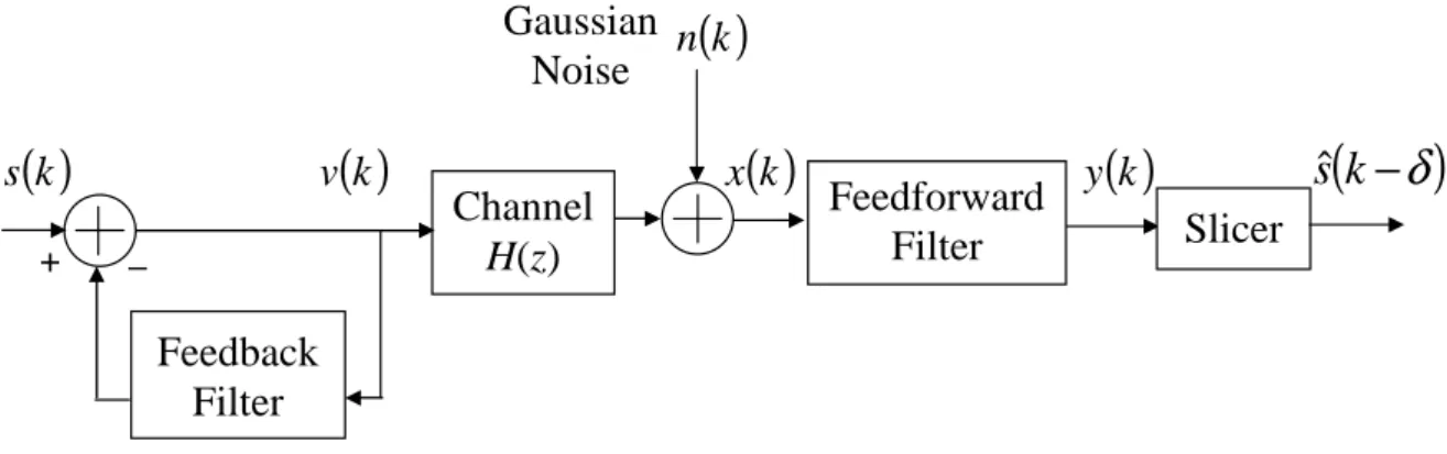
2.2 DECISION FEEDBACK EQUALIZATION AND PRE-EQUALIZATION

To remove the i.s.i. and noise, an adaptive equalizer tries to learn and invert the channel.

A widely-used structure is the decision feedback equalizer (DFE) shown in Fig. 2.2,

which comprises of a feedforward filter, a feedback filter and a threshold device. In the

DFE the sequence of observations to be equalized is applied to the feedforward filter,

and the decisions made on previously detected symbols are applied to the feedback

filter. The function of the feedback filter is to subtract out that portion of the i.s.i.

produced by previously detected symbols (often called precursors) from the estimates

of the future samples [35].

(27)

2.2 DECISION FEEDBACK EQUALIZATION AND PRE-EQUALIZATION 11

n

( )

k

x

( )

k

y

( )

k

sˆ

(

k

−

δ

)

Channel

Feedforward

Filter

Feedback

Filter

+

–

Gaussian

Noise

DFE

Slicer

Figure 2.2 Decision Feedback Equalizer

by vectors

f = [f1f2 · · · fNf]

T _b_{= [}_b

1b2 · · · bNb]

T_. _(2.3)

At time k, the feedforward filter contains the Nf channel observations, denoted by

x. During equalizer training, instead of using the slicer outputs, the actual mean-zero

i.i.d. transmitted symbolss(k) corresponding to the equalizer outputs are fed into the

feedback filter. Thus, the DFE tries to recover the symbol s(k₋δ) with propagation

delay δ, and hence the input to the feedback filter is sB = [s(k−δ −1)s(k−δ −

2) _{· · ·} s(k₋δ₋Nb)]T.

Now, the feedforward and feedback data vectors and weight vectors of the DFE can

combined as

z =



 x

−sB



 w=



 f

b



, (2.4)

yielding slicer inputy(k) =wHz, where (_·)H _{represents the Hermitian transpose. The}

feedback filter will work well provided that the decisions made by the slicer are correct.

However, if the slicer starts to give wrong estimates, then the feedback filter starts to

propagate errors, and, because of the feedback property, this error propagation starts

(28)

12 CHAPTER 2 BACKGROUND

tap weights of the DFE cannot avoid error propagation.

Wiener filter theory can be used to derive the optimum tap weights by minimizing

the mean squared error (MSE) difference between the desired signal and the received

signal [7]. Statistically, the Wiener filter depends on the autocorrelation matrix and

cross-correlation vector of the transmitted signal. For a given integer propagation delay

δ, the Wiener filter taps can be calculated using the formula

wδ=R−_δ1pδ. (2.5)

The optimum tap weights correspond to the delayδfor which the MSE is the minimum,

which is found using

δopt= arg min

1≤δ≤Nf+L−1−Nb

σ_s2₋pH_δ R−_δ1p_δ, (2.6)

where Rδ denotes the autocorrelation matrix

Rδ= E{z zH}=



 E{x x

H_} ₋_E_{_{x s}H B}

−E_{sBxH} E{sBsHB}



, (2.7)

and p_δ is the cross-correlation vector

p_δ =E_{zs∗(k₋δ)_}=



 HE{ss

∗₍_k₋_δ₎_}

−E_{sBs∗(k−δ)}



. (2.8)

As both the symbols and noise are i.i.d., it can be shown that

E_{x xH_}=σ2_sHHH +σ2_nINf E_{sBsHB}=σs2INb

E_{x sH_B_}=HE_{s sH_B_}=H

     

Oδ×Nb

σ2_sINb

O₍Nf+L−1−δ−Nb)×Nb

     

, (2.9)

(29)

2.2 DECISION FEEDBACK EQUALIZATION AND PRE-EQUALIZATION 13

MATLAB notation, we can write

E_{x sH_B_}=σ2sH(:, δ+ 1 :δ+Nb), (2.10)

where H(:, i : j) denotes the i-th through j-th rows of H. Similarly, because of the

independence of the symbols and noise, the cross-correlation vectorp_δ has the form

p_δ =



 σ

2

sH(:, δ) 0Nb×1



. (2.11)

After the training is completed, assuming a reliable reverse channel exists, a

practi-cal way of stopping error propagation in the DFE is to shift the feedback filter from the

receiver side to the transmitter side, which is possible due to the linearity of the overall

transceiver system and channel model. This results in the equalization system shown in

Fig. 2.3. If we retain the same symbol power levels fors(k), linear pre-equalization

per-forms equivalently to linear equalization at the receiver [45]. If, however, we normalize

the transmitted power, then the performance of the precoded system is degraded. This

is because the pre-equalization filter typically causes signal power enhancement at the

transmitter power amplifier. One way to avoid this signal power enhancement without

degrading the system performance is to introduce a limiter or non-linearity into the

feedback loop. This is known as precoding, which we discuss further in Section 2.4.

n

( )

k

( )

k

s

v

( )

k

x

( )

k

y

( )

k

sˆ

(

k

−

δ

)

Channel

H(z)

Slicer

Feedforward

Filter

Feedback

Filter

+ –

Gaussian

Noise

(30)

14 CHAPTER 2 BACKGROUND

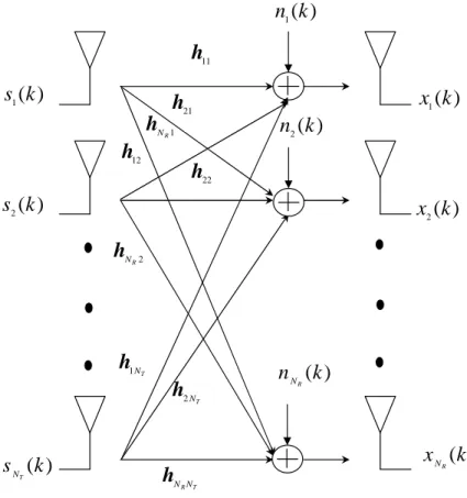
2.3 MIMO CHANNEL MODEL AND DFE

Now let us consider a more general MIMO system with NT transmitters and NR

re-ceivers. The channel between each transmitter and receiver is assumed to be a

complex-valued baseband channel. The MIMO channel model and corresponding DFE are now

presented in Sections 2.3.1 and 2.3.2.

2.3.1 MIMO Channel Model

Figure 2.4 shows a block diagram of ourNT×NRMIMO communication model. Using

)

(

1

k

s

)

(

2

k

s

)

(k

x

R N

)

(k

n

_N_R

)

(

2

k

n

11

h

21

h

1 R N

h

12

h

22

h

2 R N

h

T N 1

h

T RN N

h

T N 2

h

)

(

1

k

n

)

(k

s

T N

)

(

1

k

x

)

(

2

k

x

Figure 2.4 Block diagram of MIMO channel model

the notation of [46], the channel output at the j-th receiver (1_≤j_≤NR) at timek is

xj(k) = NT

X

i=1 ℓ_Xi−1 m=0

(31)

2.3 MIMO CHANNEL MODEL AND DFE 15

where hm

ji represents the channel impulse response between the i-th input and j-th

output, with memory (ℓi−1). Similar to the SISO model, the symbols from the i-th

transmitter si(k), i= 1, . . . , NT, are assumed to be i.i.d. with zero mean and variance

σ2

s. The additive noise at thej-th receivernj(k) is assumed to be Gaussian, i.i.d. with

zero mean and variance σ2_n. The signal and noise are again assumed to be mutually

independent.

The channel impulse response can be represented as a vector denoted by hji =

[h0_ji h1_ji _{· · ·} h(ℓi−1)

ji ]. Now, at a time k all the channel outputs can be grouped in a

vector to represent the channel output in the form

x(k) = L_X−1 m=0

Hms(k−m) +n(k), (2.13)

whereHm is theNR×NT MIMO channel matrix corresponding to them-th lag of the

MIMO channel impulse response of the form

Hm=

     

hm₁₁ hm₁₂ _{· · ·} hm₁_N_T

..

. . .. ...

hm_N_R₁ hm_N_R₂ _{· · ·} hm_N_R_N_T

     

(2.14)

ands(k) is theNT ×1 input vector at timek. HereL= maxiℓi denotes the maximum

length of all the component channel impulse responses.

2.3.2 MIMO DFE

The corresponding MIMO DFE, comprising of feedforward filters, feedback filters and

threshold devices, can be used to remove the i.s.i. and i.u.i. in a MIMO channel. Again,

let Nf and Nb represent the length of each of the feedforward and feedback filters,

respectively. We define component matrix Fm to contain the NR×NT feedforward

(32)

16 CHAPTER 2 BACKGROUND

The matrix forms of Fm and Bm are

Fm =

      fm

11 · · · fNmT1 ..

. . .. ...

fm

1NR · · · f m NTNR

     

, Bm =

      bm

11 · · · bmNT1 ..

. . .. ...

bm

1NT · · · b m NTNT

      , (2.15)

where each fm

ij denotes the m-th tap of the feedforward filter for thei-th transmitter

and j-th receiver, and eachbm

ij denotes them-th tap of the feedback filter between the

i-th and j-th transmitters. Alternatively, we can group all of the tap weights for a

particular i-th transmitter and j-th receiver (or transmitter) in the vectors

f_ij = [f_ij0 f_ij1 _{· · ·} fNf−1

ij ]T, 1≤i≤NT, 1≤j≤NR

bij = [b0ij b1ij · · · b Nb−1

ij ]T, 1≤i, j≤NT. (2.16)

Now, the equalizer output can be expressed as

y(k) = Nf−1

X

m=0

FH_mx(k₋m)₋ N_Xb−1

m=0

BH_msB(k₋m), (2.17)

where sB is the input vector to the feedback filter. During equalizer training, instead

of the slicer outputs, the corresponding transmitted data symbols,si(k), i= 1, . . . , NT,

again are fed into the feedback filters. The input vectorsBis filled with the transmitted

data symbols and has the form

sB(k) = [s1(k−δ1) s2(k−δ2) · · · sNT(k−δNT)]

T_. _(2.18)

The MIMO DFE tries to recover all the independent transmitted symbols with

propagation delay δi, which lies in the interval 0_≤δi ≤Nf +L−1 [46]. To find the

delay for each transmitter, we send an impulse from each transmitter. Each impulse

passes through NR different paths before reaching the receiver. For example, for the

MIMO DFE structure for a 2_×3 system (Fig. 2.5), if transmitter 1 sends an impulse,

then it reaches the corresponding receiver having travelled over three different channels.

(33)

2.4 TOMLINSON-HARASHIMA PRECODING 17

Slicer

) ( 2 k s ) ( 1 k

s

h

11

21

h

12

h

31

h

22

h

32

h

) ( 1 k n ) ( 2 k n ) ( 3 k n ) ( 2 k x ) ( 3 k x ) ( 1 k

x f11

21 f 12 f 22 f 13 f 23 f ) ( 1 k y ) ( 2 k y 21

b

12

b

(

1

)

1

ˆ k−δ s

(

2

)

2

ˆ k−δ s – – + + 11

b

22

b

Figure 2.5 Decision Feedback Equalizer for a 2_×3 system

third path is between h13 and f31. The net delay for transmitter 1 is then computed

using the combined channel-equalizer response due to the three channels.

Similar to the SISO case, assuming a reliable reverse channel, the feedback filters of

the MIMO DFE can be transferred to the transmitter to mitigate the error propagation

problem. But this causes signal power enhancement at the transmitter side. Again,

MIMO precoding can be used to reduce this enhancement.

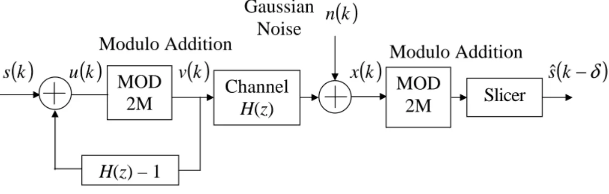
2.4 TOMLINSON-HARASHIMA PRECODING

In a THP system the equalization is done in the transmitter using an inverse modulo

filter. Therefore, error correction coding techniques can be applied in the same way

as for channels without i.s.i. Note that to construct the optimal modulo filter, the

channel transfer function needs to be known at the transmitter both for SISO and

MIMO systems.

Figure 2.6 is a general representation of a SISO THP system. The modulo adder

basically wraps around the signal constellation so that the signal does not expand

infinitely, increasing the transmit power. If the data signal is drawn from anM-point

one-dimensional PAM signal set A = _{±1,_±3, . . . ,_±(M ₋1)_}, for even M, then the

(34)

18 CHAPTER 2 BACKGROUND

( )

k

n

s

( )

k

u

( )

k

v

( )

k

x

( )

k

sˆ

(

k

−

δ

)

Channel

H(z)

H(z) – 1

Modulo Addition

Slicer

MOD

2M

Gaussian

Noise

MOD

2M

Modulo Addition

Figure 2.6 SISO Tomlinson-Harashima Precoder

Figure 2.7 shows an example plot of the function employed by the modulo adder for

M = 4. Hence, the modulo adder over a fixed interval of, say, [-M, +M) implements

−5

0

5

−4

−2

0

2

4

Input, u(k)

Output, v(k)

Figure 2.7 Output vs. input for the modulo adder

the following algorithm:

1. If the result of the summation, u(k) is greater than M, 2M is deducted from it

until it is less than M.

2. If the result of the summation, u(k) is less than -M, 2M is added to it until it is

(35)

2.4 TOMLINSON-HARASHIMA PRECODING 19

If the data symbols are drawn from anM-ary square QAM signal setA=_{a+j b_|a, b_∈

±1,_±3,_{· · ±}(√M₋1)_}, then the modulo adder makes sure that the real and imaginary

parts of the precoded symbols lie in the interval [-√M, +√M). Due to the modulo

operation, all the points spaced by integer multiples of 2√M in real or imaginary part

represent the same data.

The concept of Tomlinson-Harashima precoding (THP) for SISO channels can be

easily extended to MIMO channels. Figure 2.8 shows a generalized MIMO THP system

for a zero-forcing (ZF) system. Similar to the SISO case, the direct realization of THP

n

(k

)

v

(k

)

x

(k

)

y

(k

)

s

ˆ

(

k

−

δ

)

(k

s

MOD

2M

Channel

H(z)

H(z) - I

+ –

Decision

MOD

2M

Figure 2.8 MIMO Tomlinson-Harashima Precoder

requires advanced knowledge of the Channel State Information (CSI) matrixH(z).

One result of implementing SISO or MIMO THP is the input data is scrambled

into a pseudorandom sequence [16]. This scrambling spreads the frequency spectrum

of the data, and so reduces the intermodulation effects, but it colors the data unlike a

conventional scrambler which has a whitening effect.

As the input data sequence is modified because of the modulo addition, the receiver

needs to apply the same modulo operation to the received data to retrieve the original

transmitted symbol. Hence, the received sequence is passed through the modulo adder

(36)

20 CHAPTER 2 BACKGROUND

2.5 BLIND EQUALIZATION

Normally, for the equalizer to “learn” the channel characteristics the transmitter sends

a training sequence to the receiver, interrupting the normal transmission mode

peri-odically as the channel changes or new users join a point-to-multipoint system. But,

in a broadcast network or point-to-multipoint network a periodic training sequence

wastes valuable bandwidth for all of the users. Bandwidth is very costly, so its efficient

utilization is one of the prime factors in designing modern transmission systems.

A trained equalizer is adapted to align the output of the equalizer due to a particular

transmitted symbol with the symbol itself, and the final equalizer taps attempt to

produce the closest matching (i.e., when the difference between the equalizer output

and the desired symbol is minimum). Various kinds of algorithms such as the Least

Mean Square (LMS), Normalized Least Mean Square (NLMS) and Recursive Least

Squares (RLS) algorithms are available to minimize the mean squared error or the

least squares fit of the data to provide the best equalizer output [7].

By eliminating the need for a periodic training sequence, blind equalization

re-duces bandwidth wastage. A blind equalizer is “blind” because it does not require

any training sequence of predetermined symbols; all it utilizes are the statistical

char-acteristics of the transmitted signal. Based on these statistics, the equalizer recovers

the transmitted signal. By matching certain properties of the transmitted signal

de-rived from its higher-order statistics, many cost function-based algorithms have been

developed including the Sato algorithm, Godard-Constant Modulus Algorithm (CMA),

Multi Modulus Algorithm (MMA) and Reduced Constellation Algorithm (RCA) [8].

Each algorithm opens the “eye” of the blind equalizer, mitigating the channel distortion

of the transmitted signal.

The CMA cost function is of the form [26]:

CFCMA = E{[|y(k)|2−R2c]2}, where R2c=

E_{|s(k)_|4_}

E_{|s(k)_|2_}. (2.19)

Here,y(k) is the output of the equalizer, ands(k) is the data symbol. This cost function

(37)

2.5 BLIND EQUALIZATION 21

of radius Rc, shown in Fig. 2.9.

Figure 2.9 Graphical representation of CMA from [1]

Similarly, the MMA cost function is:

CFMMA= E{[yr2(k)−R2m]2−[yi2(k)−R2m]2}, where R2m =

E_{a4(k)_} E_{a2₍_k₎_} =

E_{b4(k)_} E_{b2₍_k₎_}.

(2.20)

Here subscriptsr andiindicate the real and imaginary parts of of the equalizer output

y(k), anda(k) and b(k) are the real and imaginary parts of the data symbol s(k). We

assume that E_{an₍_k₎_}_{= E}_{_bn₍_k₎_}_{. The cost function can be interpreted as fitting the}

output data constellation of the equalizer to a square with side lengths 2Rm. Fig. 2.10

shows its graphical representation.

Figure 2.10 Graphical representation of MMA from [1]

Finally, the RCA cost function is defined as:

CFRCA= E{|y(k)−Rrcsgn[y(k)]|2}, where R2r =

E_{a2₍_k₎_}

(38)

22 CHAPTER 2 BACKGROUND

Figure 2.11 Graphical representation of RCA from [1]

with csgn(y) = csgn(yr+jyi) = sgn(yr) +jsgn(yi), corresponding to fitting the output data constellation of the equalizer to a reduced four-point square constellation. Its

graphical representation is presented in Fig. 2.11. The equalizer tap weights can be

updated using a stochastic gradient-type recursion [1]. Note that these Bussgang-type

algorithms produce a sign ambiguity in the decoded signal. Thus, to mitigate this

problem, we assume that the transmitted signal is differentially modulated.

2.6 BLIND EQUALIZATION FOR MIMO SYSTEMS

The same algorithms can be used for MIMO systems. But, MIMO channel separation is

crucial for successful reception of the transmitted signals. The condition of

distortion-less reception for a SISO system requires that the z-transform of the system impulse

response has no zeros on the unit circle [8]. The same condition can be extended to

find necessary and sufficient conditions for the identifiability of MIMO channels [3],

[47]. We review these conditions in the following sections.

2.6.1 Condition for MIMO Channel Identification

Figure 2.12 shows an NT ×NR MIMO system with a linear equalizer at the receiver.

Setting the channel noise to zero, the linear equalizer satisfies the condition of

distor-tionless reception when

(39)

2.6 BLIND EQUALIZATION FOR MIMO SYSTEMS 23 Blind Algorithm ) ( 1 k s ) (k

sN_T

11 h T N 1 h 1 R N h T RN N h ) ( 1 k n ) ( 1k x ) (k n R N ) (k

xN_R

11 f R N 1 f 1 T N f R TN N f ) (k

yN_T

) (

1 k

y

Figure 2.12 MIMO system with linear equalizer

where F(z) and H(z) represent thez-transforms of the equalizer and channel matrix

respectively, andINT is anNT×NT identity matrix. This condition yields a

bounded-input bounded-output (BIBO) stable equalizer at the receiver. Mathematically, this

BIBO zero-forcing receiver has the form [3]

F(ejω) = [HH(ejω)H(ejω)]−1HH(ejω), for NR≥NT. (2.23)

Therefore, HH(ejω₎_H₍_ejω_{) has to be nonsingular for all} _ω _∈ _[₋_{π, π}_{]. In other}

words, a MIMO channel is identifiable if H(ejω_{) is of full (column) rank for all} _ω _∈

[₋π, π]. This implies that the number of system outputs is no less than the number of

(40)

24 CHAPTER 2 BACKGROUND

2.6.2 Initial Convergence Condition for MIMO Blind Equalizer

In this thesis, we consider Bussgang-type algorithms in particular to update the MIMO

equalizer. As already mentioned, these algorithm use the higher-order moments for the

recovery of the source data. For the linear equalizer of Fig. 2.12 the equalizer output

can be expressed as

yj(k) = NT

X

i=1

∞

X

ℓ=−∞

si(ℓ)cij(k−ℓ), j= 1, . . . , NT, (2.24)

wherecij is the combined channel-equalizer system response, corresponding to thei-th

transmitted signal and j-th output of the equalizer. The combined response is related

tohji and fij by

cij(k) = NR

X

m=1

fjm(k)⋆ hmi(k), (2.25)

where ⋆ denotes the convolution. This combined response can be used in expressing

the Bussgang-type cost functions. For the MIMO channel model, we only consider the

CMA algorithm. Analogous expressions can be derived both for MMA and RCA cost

functions.

The CMA cost function for the MIMO system can be expressed as

CFMIMOCMA = E

   NT X j=1

[_|yj(k)|2−R2c]2

 

, where R

2 c =

E_{|si(k)_|4_} E_{|si(k)_|2_} =

m4s

m2s

, (2.26)

andm4sandm2srepresent the fourth and second absolute moments of the transmitted

signal. From (2.24) and (2.26) the CMA cost function for the equalizer outputyj can

be written as a function ofcij leading to

CFMIMO_CMA = NT

X

j=1

"

−(κGm22s−m4s)

X

i,k

|cij(k)|4+κGm22s

  

X

i,k

|cij(k)|2

  

2

−κGm4s

X

i,k

|cij(k)|2+

m2 4s m2 2s # . (2.27)

(41)

2.6 BLIND EQUALIZATION FOR MIMO SYSTEMS 25

to the square of the second moment of the input signal, written as:

κ×= E{| ×(k)|

4_}

[E_{{| ×}(k)_|2_}_]2. (2.28)

In (2.27) the kurtosis is specifically for a Gaussian signal withκG= 3 for real Gaussian

signals and κG = 2 for complex Gaussian signals.1

So, if the MIMO system satisfies the distortionless reception condition (2.22) and

the length of the equalizer is double-infinite, then using Foschini’s argument [5], in [3]

it is shown that the minimum points of cost function (2.27) are

|cij[k]|2=δ[k−kd, i−i0, j−j0], for some integers kd, i0 and j0. (2.29)

The Dirac delta δ[k, i, j] is defined as

δ[k, i, j] =

 



1, ifk=i= j = 0

0, otherwise.

(2.30)

In [3] a condition for satisfactory equalizer convergence is derived, requiring the

following definitions:

• The Attainable Setfor a given equalizer is:

Ca={c:cij(k) = NR

X

m=1

X

ℓ

hmi(k₋ℓ)fim(ℓ),

X

ℓ

|fij(ℓ)|<∞}, j= 1, . . . , NT. (2.31)

• The Unique Global Minimum Set Coneis:

Ci,j,k ={c:|cij(k)|>|ci′_j′(k′)| for all i6=i′ or j6=j′ or k6=k′

andX

i,j,k

|cij(k)|<∞}. (2.32)

(42)

26 CHAPTER 2 BACKGROUND

• The Boundary of Ci,j,k is:

Bi,j,k ={c:|cij(k)|=|ci′_j′(k′)| for some i6=i′ or j6=j′ or k6=k′

andX

i,j,k

|cij(k)|<∞}. (2.33)

Using these definitions, Li and Liu prove the following theorem:

Theorem 1 If the initial equalizer parameter weights are such that the initial system response vector co _∈ Ca ∩ Ci,j,k and its output satisfies the kurtosis condition

γy

γs

>0.5, (2.34)

where

γ×=

m4×

m2 2×

−κG (2.35)

is the excess kurtosis, then for a sufficiently small step size, the equalizer will cause c

to converge to a minimum point inside Ca∩Ci,j,k. (For the case of a complex random

variable (2.35) holds if E_{×2_}_{= 0}_.)

Hence, the initial response vector co has a crucial role in the initial performance

of the blind equalizer. Note that condition (2.34) is related to our previous statement

that Bussgang-type blind algorithms only work well for non-Gaussian signals. Also,

under the stated convergence conditions CMA cost function (2.27) will converge to a

setting such that each equalizer outputyj(k), j= 1, . . .,NT, is possibly a shifted and

rotated version of the transmitted symbolsi(k), i= 1,. . .,NT.

2.6.3 Modified Bussgang Algorithms for MIMO Systems

Whether an equalizer based on cost function (2.27) can recover all of the transmitted

signals depends on the channel parameters. In a SISO system, the transmitted symbol

is corrupted by the noise and its own postcursors and precursors. But, in MIMO

systems each transmitted symbol is also corrupted by the other transmitted symbols.

(43)

2.6 BLIND EQUALIZATION FOR MIMO SYSTEMS 27

cross-correlation of the individual channel impulse responses. In [39], Papadias and

Paulraj have modified the CMA cost function for a MIMO system operating over

highly correlated frequency selective channels. They introduce the following modified

CMA cost function:

CFMIMOCMA-PP= E

   NT X j=1

[_|yj(k)|2−R2c]2

  + 2

NT

X

i,i′_=1;_i₆₌_i′ d2

X

d=d₁

|rii′(d)|2, (2.36)

whererii′(d) = E[y_i(k)y∗_i′(k−d)] is the cross-correlation between usersiand i′.

The second term of the new cost function penalizes the correlations between the

users and pushes the cross-correlation term towards zero. The parameters d1 and d2

accommodate all possible delays between theNT user signals. Using this cost function

the equalizer matrix can be updated as [39]:

F(k+ 1) =F(k)₋µ[∆b1(k)· · ·∆bNT(k)], (2.37)

where

∆j(k) = E[{|yj(k)|2−R2c}yj(k)x∗(k)] + NT

X

i′_=1;_i′₆₌_i d2

X

d=d1

rii′(d)E[y_i′(k−d)x∗(k)] (2.38)

and ∆bj is an estimate of ∆j. The estimation can be based on instantaneous values or

sample averaging. But, the estimation slows the blind equalization convergence, and

hence this algorithm is suitable for MIMO systems where the receivers are very closely

spaced, yielding very high cross-correlations.

In [3], Li and Liu have also used a cross-correlation penalty function to get rid of

the co-channel interference. Their modified CMA cost function is:

CFMIMOCMA-LL = E

   NT X j=1

[_|yj(k)|2−R2c]2

  −bo

NT

X

i,i′_=1;_i₆₌_i′

(44)

28 CHAPTER 2 BACKGROUND

wherebo≥m4s/(2m22s−m4s) andK(yi, yi′) for the case of two users can be defined as

K(y1, y2) = 1 2

−1

X

k′₌_−∞

Cum[y1(k), y∗1(k), y2(k+k′), y∗2(k+k′)]

+ 1

2

∞

X

k′₌₀

Cum[y1(k−k′), y∗1(k−k′), y2(k), y∗2(k)], for all k′ ≤k. (2.40)

The cumulant is defined as

Cum(y1, y∗1, y2, y2∗) = E[|y1|2|y2|2]−E[|y1|2] E[|y2|2]− |E[y1y2∗]|2 (2.41)

for complex random variablesyj satisfying the condition:

E[yj] = E[y2j] = 0, for j= 1,2. (2.42)

The equalizer update algorithm can be implemented for any number of users, but

here we consider only two users (i= 1,2). The algorithm for two users is [3]:

f_ijn(k) =f_ijn−1(k)₋µ_{[_|yi(n)_|2₋R2_c]yi(n)₋bozi(n)}x∗j(n−k), (2.43)

where j = 1, . . . , NR, µ is a small step size, f_ijn(k) is the k-th tap weight of the ij-th filter after then-th iteration and the zi(n)’s are given by

z1(n) =

∞

X

d=0

{|y2(n−d)|2y1(n)−E[|y2(n−d)|2]y1(n)−E[y1(n)y2∗(n−d)]y2(n−d)}

z2(n) =

∞

X

d=0

{|y1(n−d)|2y2(n)−E[|y1(n−d)|2]y2(n)−E[y2(n)y1∗(n−d)]y1(n−d)} (2.44)

In practicez1(n) andz2(n) are replaced by their empirical averages. These averages

can be easily implemented using single-pole smoothing filters, at the cost of slower

equalizer convergence speed. But, as mentioned in [3], this reduction in speed often

enables convergence even when the initial condition of (2.34) is not met.

(45)

2.6 BLIND EQUALIZATION FOR MIMO SYSTEMS 29

condition (2.34) is satisfied. Then the conventional MIMO CMA algorithm without a

penalty function should be used to minimize (2.27). The purpose of the new algorithm

is to adjust the equalizer tap weights so that the excess kurtosis condition (2.34) is

satisfied. If the initial excess kurtosis ratio satisfies the condition, then there is no need

to use the modified CMA algorithm. We now consider the union of THP and blind

(46)

(47)

Chapter 3

IMPLEMENTATION AND ANALYSIS OF THP-BLIND

EQUALIZATION

In this chapter we derive SISO and MIMO system models for the combination of THP

and blind equalization techniques. As shown in Section 2.2, the DFE is a non-linear

device with a structure which can be used both for equalization and precoding. In the

following sections we study these two operation modes. As an equalizer in the receiver,

the feedback filter of the DFE is prone to error propagation, whereas as a precoder in

the transmitter, the feedback filter does not suffer from this problem, but it increases

the signal power.

After describing the system model we study the effect of THP on the statistical

properties of the transmitted data signal. We then derive bounds on the higher-order

moments of the THP-encoded signal.

3.1 DFE-BASED PRECODING OPERATION

Figures 2.2 and 2.6 show block diagrams of the DFE and the THP, with the feedback

filter in the receiver and transmitter, respectively. If the z-transform of the channel

transfer function can be represented as H(z), then ideally the THP feedback filter in

the precoder has the form H(z)₋1 as shown in Fig. 2.6. But, for most practical

scenarios the channel transfer function is not known at the transmitter, and the tap

weights of the precoder filter cannot be derived. Fortunately, a DFE can be used to

determine practical tap weights for the precoder filter. After equalizing the channel,

the tap weights of the feedback filter of the DFE are sent back to the transmitter via

(48)

32 CHAPTER 3 IMPLEMENTATION AND ANALYSIS OF THP-BLIND EQUALIZATION

the feedback filter in the DFE is no longer needed, eliminating error propagation in the

system. Only the linear feedforward part of the equalizer is retained in the receiver.

Figure 3.1 shows the training sequence mode of a DFE. In this mode, the equalizer

can apply an adaptive algorithm or Wiener filter theory (ifH(z) is perfectly known) to

determine good tap weights. At the end of the training sequence the feedback filter tap

n

( )

k

( )

k

s

x

( )

k

y

( )

k

sˆ

(

k

−

δ

)

Training Symbol

Channel

H(z)

Feedforward

Equalizer

Slicer

Feedback

Equalizer

Error

Adaptive Algorithm

+ –

Gaussian

Noise

Figure 3.1 Training sequence mode for DFE

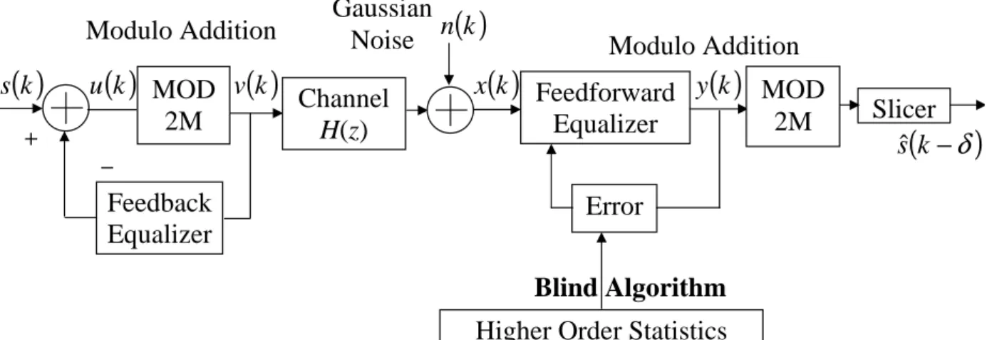
weights are transferred to the precoder, yielding only a linear equalizer at the receiver

as shown in Fig. 3.2. At this point the communication system will be in steady-state

n

( )

k

( )

k

s

u

( )

k

v

( )

k

x

( )

k

y

( )

k

(

k

−

δ

)

sˆ

Slicer

Error

Blind Algorithm

Channel

H(z)

+ –

Gaussian

Noise

Higher Order Statistics

Modulo Addition

MOD

2M

Modulo Addition

MOD

2M

Feedforward

Equalizer

Feedback

Equalizer

(49)

3.1 DFE-BASED PRECODING OPERATION 33 Error Slicer ) ( 1 k s ) ( 2 k s 11 h 21 h 12 h 22 h 32

h h31

) ( 1 k n ) ( 2 k n 13 f ) ( 3 k n 11 f 21 f 12 f 22 f 23 f 11 b 12 b 22 b 21 b ) ( 1 k y ) ( 2 k y Slicer ) ( ˆ1 k−δ

s

) ( ˆ2 k−δ

s

Feedforward Equalizer

Feedback Equalizer

Figure 3.3 Training sequence mode for MIMO DFE

mode. If, however, another user wants to join the broadcast or point-to-multipoint

system, either the initialization process has to start again or the additional user can

use an adaptive blind algorithm to deduce the tap weights of the linear equalizer while

the precoder tap weights remain fixed at the values derived from the initial training

sequence mode.

For a MIMO system, the CSI between each of the transmitter and receiver antennas

is not known beforehand in the transmitter. So, good DFE tap weights can be

deter-mined using training. Figure 3.3 shows the training sequence mode for a 2_×3 MIMO

system. Similar to a SISO system, the feedback filter tap weights can be transferred

to the transmitter via a reverse channel, and the steady state system model for the

corresponding MIMO system is shown in Fig. 3.4.

So, the operational steps for both SISO and MIMO systems can be summarized as:

1. Train the DFE to get the optimum tap weights for the feedback filter.

2. Switch from the DFE to THP, yielding only a linear equalizer in the receiver.

The feedback filter then performs the precoding operation in the transmitter.

3. Now the precoded data is passed through the channel. If another user joins the

system, a blind algorithm is used to open the “eye”.

(50)

34 CHAPTER 3 IMPLEMENTATION AND ANALYSIS OF THP-BLIND EQUALIZATION MOD 2M Slicer MOD 2M MOD 2M Slicer MOD 2M ) ( 2 k s ) ( 2 k s 11 b 11 h 21 h 12 h 22 h 32 h 31 h ) ( 1 k n ) ( 2 k n ) ( 3 k n 11 f 21 f 12 f 22 f 13 f 23 f ) ( 1 k y ) ( 2 k y ) ( ˆ1 k−δ

s

) ( ˆ2 k−δ

s ) ( 1 k x ) ( 2 k x ) ( 3 k x 12 b 21 b 22 b

Figure 3.4 Use of feedback filter of MIMO DFE in precoder

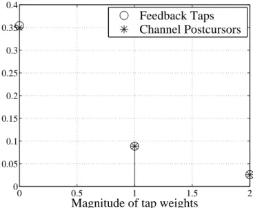
We now investigate the relationship of the feedback filter tap weights of the DFE to

the optimal THP feedback filter tap weights introduced in Section 2.4. To do this, we

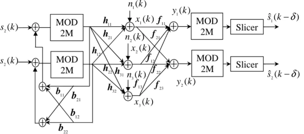
consider a simple zero channel using a DFE with Nf = 2 andNb = 1. As the channel

consists of a single zero, its length is L = 2. The z-transform of the channel impulse

response can be written as H(z) = 1 +α z−1, where α represents the single complex

zero in the channel. Thus, the transfer function of the precoder feedback filter has the

simple form α z−1. So, the THP filter in the transmitter is a one-tap finite impulse

response (FIR) filter with a single complex tap weight α.

Because we know the channel impulse response, using Wiener filter theory we can

determine the optimum tap weights of the DFE. As we will show, in the case of a

zero forcing (ZF) equalizer, the optimal tap weights of the feedback filter match the

theoretical THP tap weights. But, given channel noise, the Wiener tap weights differ

from the theoretical THP tap weights. Note that the use of THP removes the noise

enhancement problem of the ZF equalizer.

Using vector notation, the channel impulse response of the single zero channel can

be expressed ash= [1 α]. Now, the channel convolution matrixH is a 2 by 3 matrix

of the form

H =



 1 α 0

0 1 α



(51)

3.1 DFE-BASED PRECODING OPERATION 35

For this channel, we find that

E_{x xH_}=σ_s2



 1 +|α|

2 _α

α∗ 1 +_|α_|2



+σ_n2I2

E_{x sH_B_}=σ_s2



 1 α 0

0 1 α

       

0δ×1 1

0₍₂₋δ)×1

      ,

where (_·)∗ denotes the complex conjugate. Similarly, the cross-correlation vector p_δ

has the form

p_δ =σ_s2



 H(:, δ)

0



. (3.2)

For specific delayδ= 1, we have

E_{x sH_B_}=σ2s



 1 α 0

0 1 α

        0 1 0      

=σ2s

  α

1

 .

From (2.7) and (2.11) the corresponding autocorrelation matrix and cross-correlation

vector are

Rδ=1=

     

σ_s2(1 +_|α_|2) +σ2_n σ2_sα ₋σ2_sα σ2sα∗ σ2s(1 +|α|2) +σn2 −σs2

−σ_s2α∗ ₋σ2_s σ_s2

      (3.3)

p_δ₌₁=σ_s2[1 0 0]H. (3.4)

(52)

36 CHAPTER 3 IMPLEMENTATION AND ANALYSIS OF THP-BLIND EQUALIZATION

have the form

wδ=1=

     

1 0 α

0 _|_α1_|2 _|_α1_|2

α∗ _|_α1_|2

1+|α|2₊_|_α_|4

|α|2

            1 0 0       =       1 0 α       (3.5) and

f_δ₌₁= [1 0]H bδ=1=α. (3.6)

Similarly, for δ= 2 we find

E_{x sH_B_}=σ_s2



 0

α





Rδ=2=

     

σ_s2(1 +_|α_|2) +σ2_n σ_s2α 0

σ2

sα∗ σ2s(1 +|α|2) +σn2 −σs2α

0 ₋σ_s2α∗ σ2_s

    

Blind Equalization for Tomlinson Harashima Precoded Systems