An ASTER Digital Elevation Model (DEM) for the Darwin Hatherton Glacial System, Antarctica

Full text

(1)An ASTER Digital Elevation Model (DEM) for the Darwin-Hatherton Glacial System, Antarctica.. A thesis submitted in partial fulfillment of the requirements for the Degree of Master of Science in Geography in the University of Canterbury by Nita Jane Smith. University of Canterbury 2007.

(2) ii. Abstract The Darwin-Hatherton glacial system is an outlet glacial system in the Transantarctic Mountains, Antarctica, which drains ice from the East Antarctic Ice Sheet into the Ross Ice Shelf. This research provides remotely sensed data that can be used in modeling research for the Darwin-Hatherton glacial system, which in turn can be used in mass balance research for the West Antarctic Ice Sheet. Two improved digital elevation models (DEM) are produced to cover the lower Darwin Glacier and to cover the upper Darwin and Hatherton Glaciers. The new improved DEMs are generated from Advanced Spaceborne Thermal Emission and Reflection Radiometer (ASTER) satellite data, with a resolution of 45 m. To produce the two final DEMs, multiple DEMs are firstly adjusted to remove systematic errors and are then stacked and averaged to increase the accuracy and produce the final two DEMs. For the lower Darwin Glacier, 5 DEMs were averaged and in the upper Darwin and Hatherton Glaciers, 6 DEMs were averaged. The accuracy is quantified by a remaining error of + 9 m for the lower Darwin Glacier DEM and + 37 m for the upper Darwin and Hatherton Glaciers DEM. This is a significant improvement from the existing 200 m resolution Radarsat Antarctic mapping project (RAMPv2) DEM which has a remaining error of + 138 m over the lower Darwin Glacier and + 152 m over the upper Darwin and Hatherton Glaciers. The accuracy is assessed by comparing the ASTER and RAMPv2 DEMs to highly accurate ice, cloud and land elevation satellite (ICESat) laser altimetry data. A 15 m resolution, true colour, orthorectified image is provided for the entire DarwinHatherton glacial system from ASTER satellite imagery. The DEMs used to orthorectify the ASTER satellite imagery are the two new 45 m resolution ASTER DEMs. Lastly feature tracking was explored as a method for measuring surface ice velocity. This research shows that feature tracking is unsuitable for the Darwin-Hatherton glacial system if using 15 m resolution satellite imagery over a 1 to 4 year time period..

(3) iii. Contents Abstract…………………………………………………………………... ii Contents…………………………………………………………………... iii List of figures…………………………………………………………….. vi List of tables……………………………………………………………..viii Chapter 1: Introduction, aims and rationale of thesis...……...………. 1 1.1 Introduction…………………………………………………………… 1 1.2 Thesis aims and rationale..……………………………………………. 2 1.3 Thesis approach and structure…………………………….…………... 4 Chapter 2: Background and themes……………………………………. 5 2.1 Remote sensing of outlet glaciers……………………………………... 5 2.1.1 Digital elevation model extraction using remote sensing…..………………. 6 2.1.2 Ice velocity measurements using remote sensing……………………………… 8. 2.2 Climate change and its glaciological effects on the Ross Embayment.. 10 2.2.1 Ross Embayment …………..……………………………………………………… 10 2.2.2 Ross Embayment retreat and evidence from the Transantarctic Mountains. 10 2.2.3 Significance of the Ross Embayment in terms of climate change…………... 13. Chapter 3: Darwin-Hatherton glacial system………………………….. 16 3.1 Glaciology of the Darwin-Hatherton glacial system………………… 16 3.2 Previous research on the Darwin-Hatherton glacial system ………….. 18 3.2.1 Ice dynamics research……………………………..……………………………… 18 3.2.2 Glacial geomorphology research………………………………..……………... 19 3.2.3 Glacial modelling research………………………………………………………. 20.

(4) iv. Chapter 4: Remote sensing for digital elevation model generation, map generation, and ice velocity….………………………….…………. 23 4.1 Outline of the methodology…………………………………………… 23 4.2 Data sources and acquisition..………………………………………… 25 4.1.1 ASTER data ………………………………………………………………………… 25 4.1.2 ICESat data……………………………..………………………………………….. 28 4.1.3 Ground control point data…………..…………………………………………… 30. 4.3 Digital elevation model generation and accuracy validation..……….. 31 4.3.1 Generation of a DEMs………………………...…..……………………………… 31 4.3.2 Extracting ICESat and ASTER point data for accuracy validation………… 32 4.3.3 Adjusting and averaging DEMs to increase accuracy……………………….. 33 4.3.4: Validating the accuracy of the averaged ASTER DEMs……………………. 34. 4.4 Darwin-Hatherton glacial system map generation……………………. 35 4.3.1 Orthorectification of images.………..…………………………………………… 35 4.3.2 Co-registration and mosaicing of images…..………………………………….. 36. 4.5 Feature tracking for surface ice velocity……………………………... 37 4.5.1 Pre-processing of image files…………………………………………………….. 37 4.5.2 Automated feature tracking……..……………………………………………….. 38 4.5.3 Limitations causing feature tracking to fail……………………………………. 39. Chapter 5: DEM generation and a satellite image of the DarwinHatherton glacial system………………………………….………...…… 40 5.1 ASTER DEM generation by stacking and averaging….. ……………. 40 5.1.1 Individual ASTER DEMs……………….……………………………………….. 40 5.1.2 Systematic error…………………………………....……………………………… 44 5.1.3 Stacked and averaged ASTER DEMs…………….…………………………….. 46. 5.2 Validating the ASTER DEM accuracy ...………………………...……50 5.2.1 Residual error…………..…………...………..…………………………………… 53 5.2.2 Accuracy as a function of slope and elevation…….……………….……..…… 55 5.2.3 Comparison of the ASTER DEM with an existing DEM…………….……….. 57.

(5) v. 5.3 DEM summary………………………………….…………………….. 61 5.3.1 Accuracy……………………………………………………………………………. 61 5.3.2 Limitations……………………....……...…………………..……………………… 62. 5.4 An ASTER satellite map of the Darwin-Hatherton glacial system….... 63 Chapter 6: Conclusion…………………………………………………... 65 6.1 Applications of thesis data……………………………………………. 65 6.2 Recommended future research………………………………………... 66 6.2.1Recommendations for future research for DEMs………………………………. 66 6.2.2 Recommendations for future measurements of ice velocity……..…………… 67. 6.2 Final conclusion………………………………………………………..68 Acknowledgements………………………………………………………. 69 References………………………………………………………………... 70 Appendices……………………………………………………………….. 76 1: Orthorectified images for the Darwin-Hatherton glacial system………………………………………………………... 76 3: DEM generation information…………………………………… 78.

(6) vi. List of figures Figure 1.1: The Ross ice drainage system ...………………………………………………….. 2 2.1: Swinging gate model for Ross Embayment grounding line retreat since the LGM ………………………………….………………………………………………... 11 2.2: Radiative forcing components of climate change………………………………… 14 3.1: Darwin-Hatherton Glacier, Transantarctic Mountains, Antarctica……………….. 16 3.2: Field measurements of ice velocity determined from ground surveys…………..... 18 3.3: Profile of the Darwin-Hatherton Glacial System ………..………………………... 21 3.4: Modeled and measured velocities from the Darwin-Hatherton glacial system ……21 3.5: Equilibrium profiles of the Darwin-Hatherton Glacier ..…………………………. 23 4.1: Schematic flow diagram of steps to produce a DEM, a velocity contour map and a satellite map of the Darwin-Hatherton glacial system .………….……………... 24 4.2: a) Along-tack stereo satellite configuration. b) Pushbroom line scanning………... 25 4.3: Reference map for locations of ASTER images...………………………………… 27 4.4: ICESat laser altimeter data points ...…………….………………………………… 29 4.5: Location of GCPs used in this research……………...……………...……..……… 30 4.6: Systematic and residual error.. ...…………………………………………….…..... 33 4.7: Principle of co-registration…………………………………………..……………. 36 4.8: Example of offset that can occur if subsetting is not done correctly ….…………. 37 5.1: Location of lower Darwin Glacier DEMs…………………………………………. 40 5.2: Location of upper Darwin and Hatherton Glaciers DEMs………………………... 40 5.3: Raw individual DEMs for the lower Darwin Glacier……………………………... 41 5.4: Raw individual DEMs for the upper Darwin and Hatherton Glaciers…………….. 42 5.5: Location of the averaged DEMs…………………………………………………... 46 5.6: DEM of the lower Darwin Glacier at 45 m resolution……………………………. 47.

(7) vii 5.7: Raw DEM and overlap map for the lower Darwin Glacier……………………….. 47 5.8: DEM of the upper Darwin and Hatherton Glaciers at 45 m resolution…………... 48 5.9: Raw DEM and overlap map for the upper Darwin Glacier……………………….. 48 5.10: Lower Darwin Glacier: Location of total and profile ICESat points……………. 50 5.11: Upper Darwin and Hatherton Glaciers: Location of total and profile ICESat points…………………………………………………………………………………… 50 5.12: Lower Darwin Glacier DEM profile for the averaged and individual DEMs…… 51 5.13: Upper Darwin and Hatherton Glaciers DEM profile for the averaged and individual DEMs……………………………………………………………………….. 52 5.14: Histograms for elevation difference data between ASTER DEMs and ICESat elevation data: profile data……………………………………………………………... 53 5.15: Histograms for elevation difference data between ASTER DEMs and ICESat elevation data: total data……………………………………………………………….. 54 5.16: Correlation plots comparing elevation difference to slope and elevation……….. 55 5.17: Lower Darwin Glacier: Comparison between the ASTER and RAMPv2 DEMs…………………………………………………………………………………... 57 5.18: Upper Darwin and Hatherton Glaciers: Comparison between the ASTER and RAMPv2 DEMs………………………………………………………………………... 58 5.19: Lower Darwin Glacier DEM profile for ASTER, RAMPv2 and ICESat elevation data……………………………………………………………………………………... 59 5.20: Upper Darwin and Hatherton Glaciers DEM profile for ASTER, RAMPv2 and ICESat elevation data…………………………………………………………………... 59 5.21: Orthorectified, true colour, 15 m ASTER satellite map of the Darwin-Hatherton glacial system, Transantarctic Mountains……………………………………………… 64.

(8) viii. List of tables Table 2.1: Ice sheet parameters that can be measured/monitored by satellite sensors……….. 5 2.2: Selected applications of feature tracking on glaciers around the world…………... 9 2.3: Mass balance of the EAIS & WAIS………………………………………………. 13 3.1: Parameters used in glacial model……………………………..…………………... 20 4.1: Summary of all data and computer programs used in this thesis…………………. 23 4.2: ASTER characteristics…………………………………………………...………... 26 4.3: ASTER L1A reconstructed unprocessed instrument V003 data used.……………. 27 5.1: Systematic error for the ASTER DEMs……………………………………………44 5.2: Residual error for the ASTER DEMs……………………………………………... 53 5.3: Residual error comparing ASTER and RAMPv2 DEMs…………………………. 60.

(9) 1. Chapter 1: Introduction, aims and rationale of thesis 1.1 Introduction The Darwin-Hatherton glacial system (Figure 1.1) is an outlet glacial system in the Transantarctic Mountains, Antarctica which drains ice from the East Antarctic Ice Sheet into the Ross Ice Shelf. This research creates a new digital elevation model (DEM) and orthorectified satellite image for the Darwin-Hatherton glacial system and investigates whether feature tracking is suitable for measuring surface ice flow. The methodology is entirely remote sensing based using Advanced Spaceborne Thermal Emission and Reflection Radiometer (ASTER) satellite images. It is important to understand the mass balance of the Ross Embayment ice drainage system (Figure 1.1) in order to make predictions as to how the West Antarctic Ice Sheet (WAIS) may change in the future due to climate change (Bindschadler, 1998). The WAIS grounding line has been retreating since the last glacial maximum (LGM), (Conway et al., 1999), and has blocked and dammed the Darwin-Hatherton glacial system for part of this time (Bockheim et al., 1989). Understanding the lowering of the Darwin-Hatherton glacial system after the grounding ice retreated past and unblocked the outlet, allows information to be combined with other research to investigate the retreat of the WAIS. The Darwin-Hatherton glacial system is focused on as it has rarely preserved LGM glacial drifts for outlet glaciers in the southern Transantarctic Mountains (Bockheim et al., 1989). Modeling has been undertaken to investigate the LGM profile of the Darwin-Hatherton glacial system (Anderson et al., 2004), with more accurate data being required to increase the certainty of the model. Therefore this research provides a new higher quality DEM for the Darwin-Hatherton glacial system which can be used for various glaciological applications. The DEM is validated to give a reliable indication of the accuracy of the new DEM product..

(10) 2 N Antarctica. Ross Sea. Approximate Ice catchment boundary Ice Flow direction. W. East Antarctic Ice Sheet. WAIS and EAIS boundary. Ross Ice Shelf. es Ic t A e nt S h ar ee cti t c. DarwinHatherton glacial system. Ronne Ice Shelf. Figure 1.1: The Ross ice drainage system draining ice from the WAIS and EAIS into the Ross Ice Shelf.. 1.2 Thesis aim and rationale The primary aim of this thesis is to use remote sensing techniques to develop a high quality digital elevation model (DEM) for the Darwin-Hatherton glacial system, Antarctica. Specific aims are to: 1) Construct a high resolution DEM of the Darwin-Hatherton glacial system to be used for remote sensing applications. 2) Validate the accuracy of the DEM using independently measured, high accuracy laser altimetry elevation data. 3) Construct a high resolution satellite image of the entire Darwin-Hatherton glacial system. 4) Assess feature tracking as a technique to measure surface ice velocity on the DarwinHatherton Glacier..

(11) 3 The rationale for this research is to provide glacial ice surface measurements in the form of DEMs and satellite maps for the Darwin-Hatherton glacial system (Figure 3.1) so that these measurements can be used in other research to model the last glacial maximum ice thickness profile for the Darwin-Hatherton Glacier. Currently a 200 m resolution DEM of Antarctica covers the study area (www.nsidc.org, 2007). However a resolution of 200 m is too low for localised outlet glacier scale applications and has significant error (Bamber and Bindschadler, 1997). The motivation in producing a DEM with higher resolution and greater accuracy that can be used to assist in establishing the LGM profile for the Darwin-Hatherton glacial system (Figure 3.3 and 3.5), is that this glacier has a well preserved sequence of glacial drifts which can be used to validate the model used by Anderson et al., (2004). From Ross Island south along the Transantarctic Mountains there are very few ice free areas, and the extent of the Darwin-Hatherton Glacier glacial drifts is not seen elsewhere in this area. LGM profiles of outlet glaciers along the Transantarctic Mountains are used to help determine the retreat of the WAIS, using the grounding line as a marker. The grounded ice of the WAIS dammed the outlet glaciers, causing the ice profile to be much thicker at the outlet glacier terminus. When the grounding line retreated past each outlet glacier, the dam ceased and the outlet glacier thinned at the terminus. By being able to model the Darwin-Hatherton Glacier’s profile change, an age can be given for the retreat of the WAIS grounding line as it passed the Darwin-Hatherton Glacier. The Ross Ice Shelf (Figure 2.1) is the most prominent remaining ice filled marine basin on earth (Bindschadler, 1998) and it is important to understand the mass balance of the Ross Embayment ice drainage system in order to make predictions as to how the WAIS and EAIS may change in the future due to climate change..

(12) 4. 1.3 Thesis approach and structure The overall approach for this thesis involves the development of a DEM using high resolution ASTER satellite data and testing of the accuracy of this DEM. Secondary aims are achieved by using the constructed DEM for further remote sensing applications. The remote sensing techniques used are driven by the availability of suitable data for the DarwinHatherton glacial system area. ASTER imagery is the data type available which allows stereoscopy to be the DEM method and feature tracking to be the ice velocity method. The DEM accuracy is assessed from independently measured ice, cloud and land elevation satellite (ICESat) data. Feature tracking has been used on glaciers covered in features e.g. Byrd Glacier (Stearns and Hamilton, 2005). Therefore feature tracking is assessed as a method to measure ice velocity on the relatively feature free Darwin-Hatherton glacial system. Feature tracking requires an orthorectified image generated using the resulting DEM. Finally a mosaic of all orthorectified images is constructed and a satellite map of the DarwinHatherton glacial system is generated. Below is an outline of the thesis structure based on the chapters in the thesis. Chapter 2 sets the context to where this thesis fits into Antarctic science and glaciology, by presenting two research themes that underpin this research. These are are; remote sensing of outlet glaciers, and climate change and its glaciological effects on the Ross Embayment. Chapter 3 describes the Darwin-Hatherton glacial system and outlines relevant research that has been done at this location. Chapter 4 outlines the remote sensing methodology and data including; generation and accuracy validation of the DEM, generation of a satellite map, and attempting to use feature tracking to establish ice velocity. Chapter 5 presents the results and discussion. The raw DEMs are presented, adjusted, and used to generate two stacked and averaged ASTER DEMs to cover the Darwin-Hatherton glacial system. The new DEM accuracy is validating against independent ICESat elevation data and compared to an existing RAMPv2 DEM to show the improvements the new product provides. A 15 m orthorectified true colour satellite map is presented for the Darwin-Hatherton glacial system. Chapter 6 concludes this thesis by outlining the applications for this data and recommends future research for DEM generation and ice velocity measurement for the DarwinHatherton glacial system. Lastly a conclusion of thesis findings is made..

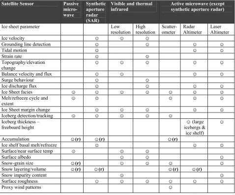
(13) 5. Chapter 2: Background and themes 2.1 Remote sensing of outlet glaciers Remote sensing of outlet glaciers is the key theme of this research. The methodological approach undertaken to achieve the aims is entirely remote sensing based. Remote sensing techniques have been successfully used in many aspects of glaciology (Table 2.1). Therefore it is important to outline remote sensing techniques used in glaciology as well as to describe the previous research and methods used for DEM generation and measuring ice flow. Table 2.1: Summary of ice sheet parameters that can be measured/monitored by satellite sensors. (r) indicates parameter still in research and development (adapted from Massom and Lubin, 2006). Satellite Sensor Passive Synthetic Visible and thermal Active microwave (except microaperture infrared synthetic aperture radar) wave radar (SAR) Ice sheet parameter Low High Scatter- Radar Laser resolution resolution ometer Altimeter Altimeter Ice velocity ☺ ☺ ☺ Grounding line detection ☺ ☺ ☺ ☺ Tidal motion ☺ ☺ ☺ Strain rate ☺ ☺ Topography/elevation ☺ ☺ ☺ ☺ ☺ change Balance velocity and flux ☺ ☺ ☺ ☺ Surge behaviour ☺ ☺ Ice discharge flux ☺ ☺ ☺ ☺ Ice Sheet facies ☺ ☺ ☺ ☺ ☺ ☺ ☺ Melt/refreeze cycle and ☺ ☺ ☺ ☺ ☺ extent Ice Sheet margin change ☺ ☺ ☺ ☺ ☺ Iceberg detection/tracking ☺ ☺ ☺ ☺ ☺ Iceberg thickness – ☺ (large ☺ freeboard height icebergs & ice shelf) Accumulation ☺(r) ☺(r) ☺(r) Ice shelf basal melt/refreeze ☺ ☺ ☺ Surface/near surface temp ☺ ☺ ☺ Surface albedo ☺ ☺ ☺ Snow-grain size ☺(r) ☺ ☺ ☺ ☺ Snow layering/volume ☺(r) ☺(r) ☺(r) ☺(r) Snow impurity content ☺ ☺ Surface roughness ☺ ☺ ☺ ☺ ☺ ☺ Proxy wind patterns ☺.

(14) 6 2.1.1 Digital elevation model extraction using remote sensing DEMs are essential in earth science remote sensing research and are used in most applications that either represent and/or analyse changes in the topography (San and Suzen, 2005). Within glaciology, DEMs are used to measure volume change which is used in understanding mass balance and ice surface deformation. DEMs of outlet glaciers and ice streams that flow into ice shelves can be used to detect the grounding line and analyse tidal dynamics (Baek et al., 2005). DEMs are also required in order to remove topographic distortion as part of pre-processing when orthorectifing raw satellite images. The resolution and accuracy of the DEM determines the application of the DEM. For example, in the interior of Antarctica a DEM with a horizontal resolution in the kilometre scale is useful for ice sheet scale applications (Bamber and Gomez-Dans, 2005), but a DEM at much higher resolution is needed for outlet glacier and ice stream scale applications. A high vertical accuracy is critical for all applications, but this is especially true for any change detection of surface height (Schenk et al., 2005). DEMs can be created by stereoscopy, photoclinometry, synthetic aperture radar (SAR) or laser and radar altimetry methods. Stereoscopy requires two images of the same area that are slightly different in viewing angle. The binocular disparity or parallax is the difference between these two images and the convergence angle between the two images determines the degree of disparity (Toutin, 2001). Clinometry uses shadows to derive elevation for specific objects, such as mountain peaks and seracs etc. This method has been applied to aerial photos and visible infra-red (VIR) satellite images (Toutin, 2001). Laser and radar altimetry and synthetic aperture radar determines surface elevation by transmitting electromagnetic radiation and measuring the reflected energy (Massom and Lubin, 2006). Laser altimetry has often been used to validate the accuracy of DEMs created by other methods (Bamber and Gomez-Dans 2005, Baek et al. 2005, Bamber et al. 2001, Bhang et al. 2007). Currently there are three DEMs that cover most of Antarctica; the Antarctic DEM from ERS1 altimetry, the RADARSat Antarctic mapping project volume 2 (RAMPv2) DEM, and the ICESat DEM (www.nsidc.org, 2007).. The Antarctic DEM from ERS-1 altimetry was. derived from radar altimetry during 1994 and 1995. This DEM has a resolution of 5 km and does not provide elevation data south of 81.5º S (Bamber and Bindschalder, 1997). The.

(15) 7 RAMPv2 DEM was constructed from a variety of sources including synthetic and airborne radar altimetry and topographic maps from the United States Geological Survey (USGS) and the Australian Antarctic Division. This DEM covers the entire Antarctic continent with variable horizontal and vertical resolution and is sampled on a 200 m grid (www.nsidc.org, 2007). Both DEMs vertical accuracy has been assessed by independent laser altimetry measurements. Large errors greater than 100 m occur in areas where data was acquired terrestrially rather than remotely. In other areas a systematic error was found. In the Antarctic DEM this error increases in a monotonic trend with slope, while in the RAMPv2 DEM this error is more complex and less predictable (Bamber and Gomez-Dans, 2005). The ICESat DEM is constructed from laser altimetry measurements from February 2003 to June 2005 and covers the Antarctic continent north of 86º S. The measurements are acquired with an along track spacing of 172 m and are interpolated to give a DEM with a resolution of 500 m DEM (www.nsidc.org, 2007). ASTER satellite imagery has been used to generate DEMs in many locations, worldwide for example Toutin 2001, Toutin and Cheng 2001, Toutin and Cheng 2002, Kaab 2001. ASTER DEM accuracy has been tested by Kaab, (2005) by comparing a 30 m resolution ASTER DEM against a 25 m resolution reference DEM generated from aerial photogrammetry for the Gruben area in the Swiss Alps (Kaab, 2001). This is an area of rough terrain, with elevations ranging from 1500 m to 4000 m, which is similar to the Darwin-Hatherton glacial system. Severe vertical errors of up to 500 m occurred in areas where steep north facing slopes existed (Kaab, 2005). These severe errors were a function of the look angle of the satellite obscuring and distorting northern faces combined with north facing slopes also being in shadow. The residual error for the ASTER DEM resulted in + 78 m standard deviation with maximum and minimum elevation differences between -220 m and 630 m. A 60 m resolution ASTER DEM was also generated and the residual error between the 30 m and 60 m resolution DEMs were compared. For elevation differences less than 100 m (approximately 90 % of sample) the 30 m DEM had greater accuracy than the 60 m DEM. However for elevation differences greater than 100 m (remaining 10 % of sample), this is reversed with the 60 m DEM having greater accuracy than the 30 m DEM (Kaab, 2005). A 30 m resolution DEM generated for an area of smoother terrain over the Gries Glacier in the Swiss Alps was also validated. The severe errors were similar but the residual error was considerably smaller with an error of + 35 m standard deviation (Kaab, 2005)..

(16) 8 2.1.2 Ice velocity measurements using remote sensing Ice velocity can be remotely sensed by either feature tracking or synthetic aperture radar interferometry (InSAR), (Table 2.2). Each method has different strengths as well as limitations. InSAR techniques use active coherent microwave radiation to illuminate the earth surface. By measuring the differences in the phase of the return radar signal from two slightly different positions twice over a short time period, both surface topography and slight changes in the surface such as ice flow can be mapped (Massom and Lubin, 2006). InSAR has a high temporal resolution in dependence of the satellite system (Massom and Lubin, 2006) . The use of microwave illumination means that cloud cover and darkness are not an issue. However, the interferogram used to establish ice velocity is limited by phase unwrapping due to phase noise and surface discontinuities such as crevasses. Excessive change in the surface over the image pair acquisition time is also a limitation as well as tropospheric and ionospheric decorrelation (Massom and Lubin, 2006)..

(17) 9 Feature tracking uses high resolution images by applying a cross correlation algorithm to identify the displacement of patterns of pixels over surface features between two images. The image time separation is determined by estimated ice velocity, image resolution, and potential surface feature distortion. Optical images have to be cloud free and the sun illumination angle has to be as similar as possible between images so that features can be consistantly identified. In addition the features must not be distorted beyond recognition. Automated feature tracking for ice flow was developed in 1991 by Bindschadler and Scambos. The main drive for this method was to allow remotely sensed velocity measurements to be undertaken in areas that have little to no bedrock exposed that could be used to co-register images such as Ice Stream E (Binschadler and Scambos, 1991). Feature tracking has been used in a number of glaciological applications around the world (Table 2.2). Table 2.2: Selected applications of feature tracking on glaciers around the world. Glacier Ice Stream E, West Antarctica. Authors Bindschadler and Scambos, (1991). Larsen Ice Shelf, Antarctic Peninsular Byrd Glacier, Transantarctic Mountains. Rack et al., (1999). Mertz Glacier, East Antarctica Daugaard Jensen Gletscher, Greenland Baltoro Glacier, Pakistan. Berthier et al., (2003) Stearns et al., (2005). Stearns and Hamilton, (2005). Mayer et al., (2006). Period Jan - Dec 1988. Satellite type Landsat 5 TM. Other information Co-registration using surface undulations relating to subglacial topography 1986-1989, 1992Landsat, ERS SAR Compared to velocity 1997 measurements at stake profiles Dec 2000 and Nov ASTER Compared to previous 2001 photogrammety velocity measurements (Bretcher, 1982) Jan 1989, Jan 2000 Landsat 5 TM, and Dec 2001 Landsat 7 ETM+ Aug 2000 and July ASTER Compared to ground 2001 velocity survey (Olsen and Reeh, 1969) 1999, 2000 and 2001 Landsat, Compared to short ASTER term GPS velocity measurements of a stake network.

(18) 10. 2.2 Climate change and its glaciological effects on the Ross Embayment Climate change and its glaciological effects on the Ross Embayment is a secondary theme of this research and underpins why research is being done in the Darwin-Hatherton glacial system within the Ross Embayment. The rationale (Section 1.2) outlines the importance of this research and how it fits into the Ross Embayment, while this section describes the Ross Embayment and previous research in more detail and outlines the significance of the Ross Embayment in terms of climate change. 2.2.1 Ross Embayment The Ross Embayment is an ice filled marine basin in Antarctica. Presently the Ross Ice Shelf covers approximately two thirds of the embayment and the remaining area varies seasonally between sea ice and open water (Figure 1.1). The Ross ice drainage system is a large complex glacial system that drains ice from approximately a quarter of Antarctica’s ice sheet surface (Denton and Hughes, 2000). Within this system ice accumulates in both the WAIS and the EAIS (Figure 1.1). The ice sheet ice flows slowly until it becomes funneled into valley type glaciers. Ice from the WAIS reaches a series of ice streams and ice from the EAIS reaches a series of outlet glaciers that flow seaward through the Transantarctic Mountains. At the point where the ice reaches the Ross Ice Shelf, the ice loses its grounding with the bedrock and becomes a floating ice shelf. 2.2.2 Ross Embayment glacial retreat and evidence from the Transantarctic Mountains The grounding line of the WAIS has been retreating southward since the LGM, but with most of the recession occurring in the middle to late Holocene (Conway et al., 1999). The grounding line was north of Cape Ross 7600 years before present and retreat has occurred in a “swinging gate” style (Figure 2.1). This implies that the southward retreat was not uniform across the Ross Embayment, but was hinged just north of Roosevelt Island. At this hinged point the slowest rate of retreat occurred, and the greatest rate of retreat occurred along the Transantarctic Mountains. In the last 7500 years the average retreat equates to 120 my-1 with similar rates still occurring e.g. the grounding line of Ice Stream C is retreating at 30 my-1 and Ice Stream B at 450 my-1 (Whillams and Bindschadler, 1988). This retreat was predetermined by major climate change at the LGM. Equilibrium has not yet been reached (Conway et al., 1999)..

(19) 11 0km. 500km 70°S. 70°S. ROSS SEA. LG M. Antarctica. gr ou nd ing. 75°S. lin e 75°S. er n s t a uth So tt Co o Sc. 7 6 0 0y r B.P. Ross Island. 3. 80°S. Roosevelt Island. 80°S. TR C TI RC TA S N AIN S A NT AN OU M. on ert ath H in rw Da cier a l G. yr B.P .P yr B 20 0. 6 80 0. Grounding line retreat evidence sites. t en es r P. n ou Gr. g din. e Lin. WEST ANTARCTIC ICE SHEET. Past extent of grounding line Present grounding line Coast line 160°W. 170°W. 180°. 170°E. 160°E. Figure 2.1: Swinging gate model for Ross Embayment grounding line retreat since the LGM with evidence from the Scott Coast, Darwin-Hatherton Glacier and Roosevelt Island (Conway et al., 1999). Evidence for this retreat has been found at three main sites. These include the Scott Coast, the Darwin-Hatherton glacial system and at Roosevelt Island. The Dry Valleys of the southern Scott Coast are an area where the Ross Ice Shelf terminated on land rather than into the ocean. Due to the landward flow of ice, proglacial lakes from the Ross Ice Sheet were dammed in the Dry Valleys. Lacustrine algae from the Dry Valleys and marine shells and seal skin from the Southern Scott Coast have been C14 dated, showing that the ice was at its approximate LGM position from at least 27,820 to 12,880 years before present, that the grounding line was still north of McMurdo Sound at 9420 years before present (Conway et al., 1999), and that open water was present at 7550 years before present. Therefore the Ross Ice Shelf must have retreated past the Southern Scott Coast between 9420 and 7550 years before present (Figure 2.1), (Conway et al., 1999)..

(20) 12 Further south along the Transantarctic Mountains the outlet glaciers’ longitudinal profiles have been controlled by WAIS grounded ice. Modeling and extrapolation of glacial drifts in the Darwin-Hatherton glacial system show that the LGM ice profile was between 800 m (Anderson et al., 2004) and 1100 m (Bockheim et al., 1989) thicker than the present ice thickness near the confluence into the Ross Ice Shelf and this LGM profile thickness thinned with distance from the confluence with the WAIS (Section 3.2.2 and 3.2.3). Algal samples from dammed lakes close to the glacier’s present level suggest that the grounding line of the Ross Ice Shelf had retreated past the outlet between 6020 and 9429 years before present (Bockheim et al., 1989), (Figure 2.1). The Darwin-Hatherton glacial system is the focus of this research. Roosevelt Island is a grounded dome of ice with the grounding line approximately 200 m below sea level surrounded by the floating ice of the Ross Ice Shelf. Research investigating bump-amplitude profiles within the ice stratigraphy are combined with ice flow models and show that divide flow first started 3200 years before present (Conway et al., 1999). It is suspected that divide flow began before the ice was fully ungrounded suggesting that the grounding line was still north of Roosevelt Island at 3200 years before present (Conway et al., 1999), (Figure 2.1)..

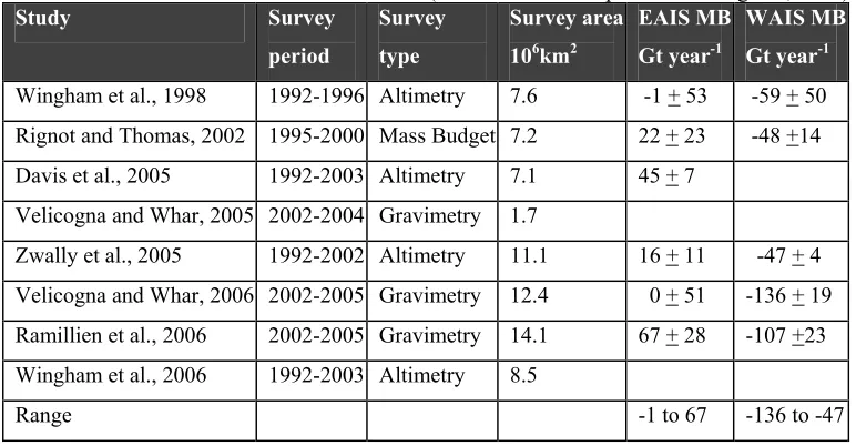
(21) 13 2.2.3 Significance of the Ross Embayment in terms of climate change Glaciers and ice sheets provide one of the most visible indications of the effects of climate change, as the mass balance of the system is determined by climatic controls (IPCC, 2007). It is important to have accurate measurements for the mass balance of the WAIS, EAIS and the total Antarctic Ice Sheet to help understand climate change. By understanding the link between climate change and mass balance we can help predict the effects that climate change may have on the ice sheets in the future. Currently estimates of Antarctic mass balance vary (Table 2.3). Table 2.3. Mass balance of the EAIS and WAIS (Modified from Shepherd and Wingham, 2007). Study Survey Survey Survey area EAIS MB WAIS MB period. type. 106km2. Gt year-1. Gt year-1. Wingham et al., 1998. 1992-1996 Altimetry. 7.6. -1 + 53. -59 + 50. Rignot and Thomas, 2002. 1995-2000 Mass Budget 7.2. 22 + 23. -48 +14. Davis et al., 2005. 1992-2003 Altimetry. 45 + 7. 7.1. Velicogna and Whar, 2005 2002-2004 Gravimetry. 1.7. Zwally et al., 2005. 11.1. 16 + 11. -47 + 4. Velicogna and Whar, 2006 2002-2005 Gravimetry. 12.4. 0 + 51. -136 + 19. Ramillien et al., 2006. 2002-2005 Gravimetry. 14.1. 67 + 28. -107 +23. Wingham et al., 2006. 1992-2003 Altimetry. 8.5 -1 to 67. -136 to -47. Range. 1992-2002 Altimetry. There are two main reasons for this variation. First, there are three main methodological approaches which have different systematic method errors (Shepherd and Wingham, 2007). Secondly, there is uncertainty associated with the lack of complete data for remote locations which causes best estimates to be used in modeling. Currently in Antarctica there are very little glaciological data specifically for outlet glaciers along the southern Transantarctic Mountains..

(22) 14 The need to quantify and understand the mass balance of ice sheets has become increasingly important. This need is due to increased understanding of the impacts of anthropogenic enhanced climate change. The most recent report produced by the IPCC states that the global atmospheric concentrations of carbon dioxide, methane and nitrous oxide (Figure 2.2) have increased markedly as a result of human activities since 1750 and now far exceed pre-industrial values with a radiative forcing of + 1.6 Wm-2 (+0.6 to +2.4) (IPCC, 2007).. Long lived greenhouse gases. CO2. CH4, N20 Halocarbons. Anthropogenic. Ozone Water vapour Surface albedo Aerosol direct affect Aerosol cloud albedo effect Linear contrails. Natural. Solar irradiance Total anthropogenic. -2. -1 0 1 Radiative Forcing (Wm-2). Figure 2.2: Radiative forcing components of climate change (modified from IPCC, 2007). 2.

(23) 15 Some of the direct observations of this positive radiative forcing are: an increased surface temperature of 0.76 ºC with uncertainty of 0.57º to 0.95 ºC since 1850, an increased troposphere temperature, an increased water vapor, a decrease in the size of the Arctic sea ice, a decrease in mountain glaciers/snow, a 7 % loss of northern hemisphere permafrost since 1900, regional changes in precipitation, and an average sea level rise of 1.8 mmyr-1 (uncertainty of 1.3 - 2.3mmyr-1) since 1961 (IPCC, 2007). The IPCC also states that this change may cause “a probable decrease in the ice sheets of Greenland and Antarctica” and “Current global model studies project that the Antarctic Ice Sheet will remain too cold for widespread surface melting and is expected to gain in mass due to increased snowfall. However, net loss of ice mass could occur if dynamic ice discharge dominates the ice sheet mass balance” (pg 17, Fourth assessment report of the IPCC, 2007). Despite the uncertainty there is concern about the stability of the WAIS. Theoretical analysis suggests that ice-filled marine basins are unstable and current predictions show continued grounding line retreat and loss of volume. Two different retreat models, a linear retreat, and an accelerated retreat predict that the grounding line would reach the West Antarctic ice divide by 7000/4000 years respectively with 0.8/1.3 mmyr-1 sea level rise respectively (Bindschadler, 1998a). Therefore further research needs to be undertaken in order to provide mass balance measurements with less uncertainty so that they can be used to validate the WAIS retreat models..

(24) 16. Chapter 3: Darwin-Hatherton glacial system 3.1 Glaciology of the Darwin-Hatherton glacial system The Darwin-Hatherton glacial system is an Antarctic outlet glacial system located within the Transantarctic Mountains between 155º and 161 ºE longitude, and between 79º and 80 ºS latitude (Figure 3.1). N. 0. 50 100km. 158°0’ 00” E. 157°0’ 00” E. 156° 0’ 00” E. 159°0’ 00” E. 160° 0’ 00” E. 0 Te dg Ri e. Up pe rD ar wi n. 20km. Scale. le ac nt. Ross Ice Shelf. 10. 161°0’ 00” E. G lac i. er. 79°45’ 00” S. Ross Ice Shelf. Brow n Hills Diam ond Hill. ng. lin e. Low er er ac i Darwin Gl. Glac ie r. Gr ou nd i. Ha the r to n. Darw in Mountains. Junction Spur. Britannia Range. ss Ro. rd By. Ic e. ac Gl. elf Sh. ier. Figure 3.1: Darwin-Hatherton Glacier, Transantarctic Mountains, Antarctica. Light blue lines show glacier flow and brown areas are ice free areas (modified from ST 57-60/13* map, Antarctica 1:250,000 Reconnaissance Series, USGS, 1963.. The geomorphology of the Transantarctic Mountains in this area is a function of mountain uplifting processes through a pre-existing ice sheet (Denton, 1979). As the mountains were uplifted ice carved out valleys, isolating nunataks. Over time valleys with geologic weaknesses became the predominant drainage valleys for the interior EAIS leaving other transverse valleys to have glaciers that were smaller and slower moving. The smaller and slower glaciers are widespread along the Transantarctic Mountains and make up a significant. 80°0’ 00”S.

(25) 17 part of the EAIS drainage system in the Transantarctic Mountains. The Darwin-Hatherton glacial system is an example of a smaller, slower moving glacier. The bed profile of the Darwin-Hatherton glacial system is currently unknown. The Darwin-Hatherton glacial system has two main accumulation areas; the upper Darwin Glacier and the upper Hatherton Glacier (Figure 3.1). Four other smaller catchments provide ice to the system, three of which drain from the Britannia Range, and a fourth that is separated from the upper Darwin Glacier by Tentacle Ridge. Most of the glacier surface comprises pf “blue ice”. The features on the ice surface include: supra-glacial melt water ponds and channels on the lower Darwin Glacier, medial moraines and flow bands in the upper Hatherton and lower Darwin glaciers, and crevasse fields in the upper Darwin Glacier and pockets of supra-glacial moraine in the upper Hatherton Glacier. The Darwin-Hatherton glacial system is grounded and the Ross Ice Shelf is floating. Therefore as the glacier flows out onto the ice shelf the glacier becomes ungrounded. Hughes and Fastook (1981) inferred the position of the grounding line for the neighbouring Byrd Glacier from a break in elevation and velocity in the glacier at approximately 200 m above sea level. Tidal response was also measured, and supports this inference (Hughes and Fastook, 1981). Because of the close proximity it can be inferred that the Darwin-Hatherton Glacier grounding line will be similar in elevation to the Byrd Glacier. Surface ice velocity measurements have been measured once by field surveying in 1981 by Hughes and Fastook (Section 3.2.1). Theoretical calculations of the basal temperature using the Quadrature method (Hindmarsh, 1999) for the Darwin-Hatherton glacial system were conducted for the purpose of modeling (Anderson et al., 2004). These calculations established that part of the base may be above the pressure melting point. The mass balance for the Darwin-Hatherton glacial system is currently only estimated from hypothetical modeling (Section 3.2.3), verified by sparse field measurements (Section 3.2.1). Until velocity data, volume data and input/output data are measured the mass balance can not be calculated accurately. There are currently very sparse meterological data available for this area but estimates of accumulation in the Polar Plateau and Ross Ice Shelf are 0.10 to 0.15 gcm-2y-1 and 20 gcm-2y-1 respectively and annual average temperatures of -35º to -40 ºC and -30 ºC respectively (Bockheim et al., 1989). The microclimate of the Darwin Glacier and the Hatherton Glacier are different with the Polar Plateau winds affecting the Hatherton Glacier more than the Darwin Glacier (Bockheim et al., 1989)..

(26) 18. 3.2 Previous research on the Darwin-Hatherton glacial system The Darwin-Hatherton glacial system is a remote, bordering deep field location of Antarctica (Figure 3.1) and there has been limited research done at this location. This section reviews all glaciological and glacial geomorphological research undertaken in the Darwin-Hatherton glacial system to date. 3.2.1 Ice dynamics research Velocity has been sparsely measured by Hughes and Fastook (1981), (Figure 3.2). However this research was predominantly based on the neighbouring Byrd Glacier where ice flow research was undertaken initially by field measurements (Hughes and Fastook, 1981), and then subsequently aerial photograph sets were used to undertake a photogrammetry ice flow study (Brecher, 1982) validated by the initial field measurements. The aim of this research was to provide data that could be used to create a finite-element analysis of the Byrd-Ross Ice Shelf interaction. 65 markers were surveyed on the Byrd Glacier and 6 on the DarwinHatherton glacial system. The velocities of the Darwin-Hatherton Glacier ranged from approximately 75 my-1 above Junction Spur (Figure 3.2) to between 75 my-1 and 200 my-1 on the lower Darwin-Hatherton glacial system (Figure 3.2). East Antarctic Ice Sheet. Up p. er Da rw in. G. la ci er. Ross Ice Shelf. th Ha. 0. 0.2. 0.4 0.6 0.8. ice velocity (km/year) 0. 5. 10. 15. 20. to er. n. r ie ac Gl. n wi ar D r we r Lo cie a Gl. ss Ro. S Ice. lf G he. din un ro. in gl. e. r cie Gla d r By. scale (km). Figure 3.2: Field measurements of ice velocity determined from ground surveys. (modified from Hughes and Fastook, 1981).

(27) 19 3.2.2 Glacial geomorphology research Geomorphological research has been undertaken in the Hatherton glacier area (Bockheim and Wilson 1979, and Bockheim et al. 1989), based on the well preserved glacial lateral drifts that are remnants of past glacial regimes in the area. Soil properties were used as relative age indicators and stratigraphic markers to separate out the different lateral drifts and compare to McMurdo Sound sequences (Bockheim and Wilson, 1979). Longitudinal ice surface profiles were constructed for each of the different drifts (Bockheim et al., 1989). The LGM profile is well constrained in the Hatherton Valley but is extrapolated downstream of Junction Spur due to lack of distinct boundaries. The Britannia drift shows that at the Last Glacial Maximum the ice thickened above the present level by (Figure 3.3) by 100 m at the inland extremity, 450 m mid glacier, and by 1100m at the confluence of the glacier to the Ross Ice Shelf (from extrapolated data).. 4000. Present Ice Surface LGM Ice Surface, dotted where extrapolated. Bibra Valley. Isca Valley. Lake Wellman. 1500. Tentacle Ridge. 2000. Diamond Hill. Ross Ice Shelf. 2500. Dubris Valley. Elevation above sea level (m). 3000. Darwin Nunatak. 3500. 1000 500 0. 0. 25. 50. 100. 125. Distance from Ross Ice Shelf (m). Figure 3.3: Profile of the Darwin-Hatherton Glacial System showing the present ice surface and ice surfaces from the past (Bockheim et al., 1989). C14 dating techniques were used to give a basic age control on ice recession. Algae from former kettle and glacier dammed lakes were used to give a minimum age for recession. The Britannia/LGM drift is dated to between 9420 years and 10,250 years before present and the ice surface was close to its present level between 5740 years and 6020 years before present (Bockheim et al., 1989), indicating that the grounding line of the WAIS retreated past the Darwin-Hatherton glacial system between 6020 years and 9420 years before present.

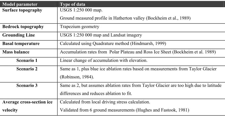
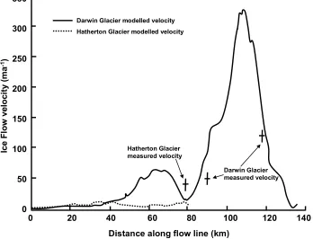
(28) 20 3.2.3 Glacial modeling research By using the geomorphological research as validation (Chapter 3.2b), modeling research was used to a) model the elevation of ice at the Darwin Glacier/Ross Ice Shelf confluence at the LGM and, b) model the time for the Darwin-Hatherton glacial system to respond to the retreat of the WAIS grounding line (Anderson et al., 2004). The model is a simple one-dimensional flow line model where an average ice velocity is passed through a trapezium transverse valley cross-section (no longitudinal stresses taken into account). Some of the parameters used in the model are taken from sparse measured data and others are based on glacial theories (Table 3.1). Table 3.1: Parameters used in glacial model (from Anderson et al., 2004) Model parameter Surface topography. Type of data USGS 1:250 000 map. Ground measured profile in Hatherton valley (Bockheim et al., 1989). Bedrock topography. Trapezium geometry. Grounding Line. USGS 1:250 000 map and Landsat imagery. Basal temperature. Calculated using Quadrature method (Hindmarsh, 1999). Mass balance. Accumulation rates from Polar Plateau and Ross Ice Sheet (Bockheim et al. 1989). Scenario 1. Linear change of accumulation with elevation.. Scenario 2. Same as 1, plus blue ice ablation rates based on measurements from Taylor Glacier (Robinson, 1984).. Scenario 3. Same as 2, but assumes ablation rates from Taylor Glacier are too high due to latitude differences and reduces ablation to fit.. Average cross-section ice. Calculated from local driving stress calculation.. velocity. Validated from 6 ground measurements (Hughes and Fastook, 1981). The modeled velocity was validated against 5 velocity measurements (Hughes and Fastook, 1981). The values used in calculating the cross section ice velocity (Table 3.1) were not well established and were used as tuning parameters. The modeled ice velocity matches the measured ice velocity reasonably well with a difference in values of between 10-20 ma-1 (Figure 3.4).

(29) 21 350 Darwin Glacier modelled velocity. Ice Flow velocity (ma-1). 300. Hatherton Glacier modelled velocity. 250 200 150 100. Hatherton Glacier measured velocity Darwin Glacier measured velocity. 50 0. 0. 20. 40. 60. 80. 100. 120. 140. Distance along flow line (km). Figure 3.4: A comparison between modeled and measured velocities from the Darwin-Hatherton glacial system (Anderson et al., 2004).. 2000 1500 1100m. Elevation (m). 1000. 800m. 500 100m. 0. -500. Wet glacier bed Dry glacier bed Present glacier surface. -1000. LGM surface from field research Extrapolated LGM surface LGM surface from best fit modelling research. -1500 0. 50. 100. 150. Distance along flow line (km). Figure 3.5: Equilibrium profiles of the Darwin-Hatherton Glacier showing present day profile, as well as modeled and measured LGM profiles (modified from Anderson et al., 2004).

(30) 22 The model equilibrium profiles were validated against the LGM profile (Bockheim et al., 1989). The best fit model suggests a LGM outlet profile elevation of 800 m above the present Ross Ice Shelf. The extrapolated LGM profile suggests an 1100 m elevation above the present Ross Ice Shelf (Figure 3.5). Therefore there is a 300 m discrepancy between the two different methods. However the two profiles match well at the junction of the Darwin and Hatherton Glaciers. The response time between the retreat of the WAIS grounding line and the DarwinHatherton glacial system reaching equilibrium was modeled as a linear retreat and as a stepwise with a response time of 300 years and 1100 years respectively. Geomorphological research gives a window of 3400 years (Bockheim et al., 1989) for this to have happened, so both modeled scenarios fit within this window. Due to the lack of measured data that were fed into this model there have been many assumptions made and the potential uncertainty is high. Currently surface velocity, bedrock profiles, atmospheric parameters and paleo-thickness measurements are being studied further. These can then be used to place greater certainty on this model..

(31) 23. Chapter 4: Remote sensing for digital elevation model generation, map generation, and ice velocity 4.1 Outline of the methodology The aims of this thesis were achieved in four main stages (Figure 4.1). 1) Suitable satellite data and ground control points (GCPs) were chosen and acquired; ASTER satellite imagery, ICESat satellite elevation data and GPS and topographic ground control points (Section 4.2). 2) Individual DEMs were generated for each ASTER image, systematic errors were removed and the precision of the DEMs was increased by stacking and averaging individual DEMs. ICESat elevation data were used to assess the DEM accuracy (Section 4.3). 3) Orthorectification using the DEM and the raw ASTER images and further preprocessing were used to generated a true colour, 15 m resolution satellite map of the Darwin-Hatherton glacial system (Section 4.4). 4) The individual orthorectified ASTER images were further processed and feature tracking techniques were applied in an attempt to establish whether feature tracking using ASTER data could be used to measure the ice surface velocity of the DarwinHatherton glacial system (Section 4.5). Table 4.1: Summary of all data and computer programs used in this thesis Data source Use ASTER image data Create DEM and satellite map Ground control points Assist in DEM creation ICESat data Validate ASTER DEM Computer Program Use ERDAS Imagine Lieca • DEM generation. Photogrammetry Suite • File conversion ENVI 4.3 • Orthorectification. • Co-registration. • Sub-setting. • Averaging DEMs. • Mosaicing ArcGIS • Gain ground control point data from USGS topographic maps. • Extracting ICESat data • Presenting maps IMCORR • Feature tracking.

(32) Run feature tracking. Subset images. Generate orthorectified mosaic map. Co-register orthorectified images together. Generate orthorectified image. elevation data to assess DEM accuracy. Use independent ICESat. Generate reference DEM (Ave of all DEMs). Generate individual image DEMs. Choose & acquire data & software. IMCORR. ENVI. ENVI. ENVI. ENVI. ENVI. ERDAS. DEM. ASTER 2002 L.D. Orthorectified 2002 L.D. U.D velocity. 2002U.D. 2002 L.D L.D velocity. 2001U.D. Mosaic orthorectified map. 2002U.D Co-reg. Orthorectified 2002 U.H. DEM. ASTER 2002 U.H. U.H velocity. 2002U.H. 2001U.H. 2002U.H Co-reg. 2001U.H. Orthorectified 2001 U.H. DEM. ASTER 2001 U.H. Average DEM for U.D & U.H. Orthorectified 2002 U.D. DEM. ASTER 2002 U.D. 2001U.D. Orthorectified 2001 U.D. Graphs showing DEM accuracy. ICESat elevation. DEM. ASTER 2001 U.D. 2001 L.D. 2002L.D Co-reg. 2001L.D. Orthorectified 2001 L.D. Average DEM for L.D. DEM. ASTER 2001 L.D. Figure 4.1: Schematic flow diagram showing progression of steps required to produce a DEM, a velocity contour map and an accurate map of the Darwin/Hatherton glacial system using remote sensing .For simplicity, only data sets, 2001 and 2002 are shown in this diagram. Red = Data source, Blue = Processing step, Green = Result, L.D = lower Darwin, U.D = upper Darwin, U.H = upper Hatherton. 4. 3. 2. 1. 24.

(33) 25. 4.2 Data sources and acquisition. 4.2.1 ASTER data Satellite imagery data from the Advanced Spaceborne Thermal Emission and Reflection Radiometer (ASTER) sensor were used. The ASTER sensor is aboard the Terra Satellite and is run co-operatively by NASA and Japan’s Ministry of Economic Industry (Elachi and van ZYL, 2006). Terra was launched on 18 December 1999 (Richards and Jia, 2006). The Terra Satellite has a near polar orbit and is sun-synchronous. The images are acquired by a multispectral imager that operates by pushbroom line scanning in the along track direction (Figure 4.2b) with three telescopes, covering 15 bands from the visible to the thermal infrared spectral region (Table 4.2). Of the 15 bands, the 3n and 3b bands (Table 4.2) acquire images with slightly different look directions (Figure 4.2a) and by combining the two slightly different bands, stereoscopy can be used to create a DEM (Elachi and van ZYL, 2006). ASTER data have been used successfully used to create DEMs for many applications and have been successfully used to determine ice velocity from feature tracking (Stearns and Hamilton 2005, Stearns et al. 2005, Mayer et al. 2006). Time C Signal out. Time B. Time A. Linear detector array with one detector per pixel across the swath. Satellite track Field of view. Nadir. Platform motion sweeps out an image. Nadir Ground track. a). b). Figure 4.2: a) Along-tack stereo satellite configuration showing both forward and backward (3n and 3b) band look angles, which are acquired during one overflight with a time difference of seconds to minutes (modified from Kaab, 2005). b) Pushbroom line scanning in the along-track direction (Richards and Jia, 2006).

(34) 26 Table 4.2: ASTER characteristics (modified from Elachi and van ZYL, 2006 and Richards and Jia, 2006) Subsystem Band no. Spectral range Spatial Swath Quantization (µm) resolution(m) (km) levels (bits) VNIR 1 0.52-0.60 15 60 8 2 0.63-0.69 15 60 8 3n 0.78-0.86 15 60 8 3b 0.78-0.86 15 60 8 SWIR 4 1.60-1.70 30 60 8 5 2.145-2.185 30 60 8 6 2.185-2.225 30 60 8 7 2.235-2.285 30 60 8 8 2.295-2.365 30 60 8 9 2.360-2.430 30 60 8 TIR 10 8.125-8.475 90 60 12 11 8.475-8.825 90 60 12 12 8.925-9.275 90 60 12 13 10.25-10.95 90 60 12 14 10.95-11.65 90 60 12. Stereo Pair. Eleven ASTER images were chosen from three different times; December 2001, 2002, and 2005 (Figure 4.3 and Table 4.3). Data time periods were chosen to provide the most up to date DEM, satellite map, and ice velocity measurements as well as choosing a time separation designed to balance out two factors when attempting feature tracking; a long enough time period to reduce the proportion of pre-processing error, and b) a short enough time period to reduce the distortion of identifiable features for feature tracking. Images acquired at similar times of year reduce seasonality issues such as snow cover and sun illumination angle. Choosing a similar time of day was considered in order to reduce illumination differences. Due to the small set of good quality images, this level of selection was not possible. The range in quality of ASTER images is primarily due to cloud cover. Therefore images were chosen and acquired with less than 10 % cloud cover. Image data were acquired through the USGS NASA Land Processes Distributed Active Archive Centre (LPDAAC) website (www.LPDAAC.usgs.gov, 2007). The images were in LIA format, which is the raw and unprocessed format that has no projection information requiring a DEM in order to correct for topographic error. For this research the given projection was UTM, spheroid and datum WGS84, and zone 57 south. Image codes for three images from 2001, six from 2002 and two from 2005 can be seen in table 4.3. The location with 5 images covering the lower Darwin Glacier and 6 images covering the upper Darwin and Hatherton Glaciers can be seen in figure 4.3..

(35) 27. Figure 4.3: Reference map for locations of ASTER images, with colour indicating year of acquisition. Table 4.3: ASTER L1A reconstructed unprocessed instrument V003 data for imagery used in this research. First two numbers of the code = the acquisition year, LD = Lower Darwin, UD = Upper Darwin, UH = Upper Hatherton. Image Data Code. Code. Date. Time. Latitude (South). Longitude. SC:AST_L1A:003:2006010384 SC:AST_L1A:003:2006010385 SC:AST_L1A:003:2008836878. 01UD 01UH 01LD. 22 Dec 2001 22 Dec 2001 29 Dec 2001. 20:11:00 20:11:09 15:23:47. 79.89 79.61 79.85. 155.63 158.24 159.91. SC:AST_L1A:003:2010110024 SC:AST_L1A:003:2009693791 SC:AST_L1A:003:2010110023 SC:AST_L1A:003:2009629930 SC:AST_L1A:003:2009693792 SC:AST_L1A:003:2009629920. 02LDa 02LDb 02UHa 02UHb 02UHc 02UD. 04 Dec 2002 09 Dec 2002 04 Dec 2002 07 Dec 2002 09 Dec 2002 07 Dec 2002. 19:51:01 20:09:27 19:51:09 20:21:48 20:09:36 20:21:39. 79.83 79.83 80.09 79.84 80.12 79.54. 160.08 159.05 157.36 155.97 156.41 158.46. SC:AST_L1A:003:2032605958 SC:AST_L1A:003:2032304483. 05LDa 05LDb. 05 Dec 2005 18 Dec 2005. 14:49:16 20:49:46. 79.88 79.83. 159.35 160.01.

(36) 28 4.2.2 ICESat satellite data Data from the geoscience laser altimeter system (GLAS) on the NASA ice, cloud and land elevation satellite (ICESat) were used to validate the quality of the ASTER generated DEM. ICESat has been used in Antarctica to study elevation changes of ice sheets, outlet glaciers and ice streams (Baek et al. 2005, Csatho et al. 2005, Nguyen and Herring 2005, Schenk et al. 2005) and to validate DEMs generated from other data (Baek et al. 2005, Bamber and Gomez-Dans, 2005). The laser altimeter pulses energy with a wavelength of 1064 nm at 40 Hz, and the echo pulse is received by a telescope with a 1 m diameter (Schutz et al., 2005). The laser illuminating footprint on the earth surface is ~65 m in diameter and each elevation measurement spot has a successive along-track spacing of 172 m (Schutz et al., 2005). The ICESat mission was launched in 2003 with a primary purpose of providing data to analyse polar ice sheet volume change with an accuracy of greater than 2 cmyr-1 (Schutz et al., 2005) to be combined with mass balance and sea level rise research. ICESat accuracy studies using ground based GPS surveys in Bolivia (Fricker et al., 2005), and independent terrain models from the NASA airborne terrain mapper in the USA and Dry Valleys of Antarctica (Martin et al., 2005), give an absolute accuracy in elevation of ~2 cm. Timing accuracy has been validated to microsecond level (Magruder et al., 2005)..

(37) 29 The Antarctic and Greenland ice sheet data product (GLA12) from Laser 2a was used in this research. The GLA12 data were acquired between October and November, 2003 (Figure 4.4) and obtained through the National Snow and Ice Data Centre (NSIDC) at the University of Boulder, Colorado. The accuracy of GLA12 data over the Antarctic and Greenland ice sheets has been shown to have a systematic error of 9.6 cm and a standard deviation corresponding to the residual error of + 4.9 cm (Brenner et al., 2007).. N. Figure 4.4: ICESat laser altimeter data points available for the Darwin-Hatherton glacial system (shown by white points that make the white lines), overlaid on an ASTER DEM of the area..

(38) 30 4.2.3 Ground control point data Ground control points (GCPs) were determined in order to create a DEM and to orthorectify the ASTER images. To provide satellite imagery over the entire Darwin-Hatherton glacial system, at least three ASTER images with a 60 km x 60 km area were required. Therefore at least one GCP was required to use for each image. The Darwin-Hatherton glacial system is remote and there is a lack of GCPs available. GCPs were acquired in two different ways, both using the datum WGS84. In the lower Darwin Glacier, GPS points were taken in the field in January 2007 using a Garmin 72 GPS, and WGS84 datum. One GPS point was at a site near the terminus of the Foggydog Glacier (Figure 4.5) and was able to be located on the ASTER images with an estimated accuracy of + 3 pixels (45 m). The GPS point had a horizontal accuracy of + 11.4 m and was not differentially corrected. In the upper Darwin and upper Hatherton Glaciers, GCPs were obtained from a digitised version of the 1963 ST 57-60/13* topographic map from the Antarctica 1:250,000 Reconnaissance Series (USGS, 1963). The digitised maps had point elevation data available for high points in ice free areas (Figure 4.5). These points were approximately located onto the ASTER images by assuming that the points corresponded to the highest point in the area of which they were extracted from on the digitised map. The elevation data were extracted from the USGS maps and located onto the ASTER images using ArcGIS. N. 0. 50 100km. 156°0’00” E. 157°0’00” E. 158°0’00” E. 159°0’00” E. 160°0’00” E 0. 10. 161°0’00”. 20km. Scale. Ross Ice Shelf. Tentacle Ridge 79°45’00” S. Junction Spur. Foggydog Glacier terminus. 80°0’00”S. Figure 4.5: Location of GCPs used in this research. Yellow dots indicate approximate location of GCP. Foggydog Glacier terminus GCP was acquired from hand held GPS measurement. Junction Spur and Tentacle Ridge GCPs were acquired from the digitised ST 57-60/13* Antarctica 1:250,000 Reconnaissance Series map (USGS, 1963)..

(39) 31. 4.3 Digital elevation model generation and accuracy validation 4.3.1 Generation of DEMs Stereoscopy techniques were used to construct DEMs for each raw ASTER image using the ERDAS Lieca Photogrammetry Suite. Each ASTER multispectral image contained a stereo image pair in the visible near infra red (VNIR) spectral range. The stereo image pair was of near identical image areas acquired from slightly different look angles and was used along with GCP to construct a DEM. Images covering the lower Darwin Glacier used one GPS GCP (Figure 4.5), and images covering the upper Darwin and Hatherton Glaciers used a USGS topographical map GCP (Figure 4.5). The DEM resolution was 45 m due to the limitations of the software requiring the minimum pixel size to be three times the resolution of the original image pixel size. This is due to the number of GCPs available. A one pixel (15 m) resolution DEM has previously been created from ASTER imagery (San and Suzen, 2005), but 30 to 60 GCPs were used. For each stereo image pair, GCPs and tie points were located so that triangulation could be achieved. Once the GCPs were located, 5 - 10 tie points were manually located allowed automatic tie point generation to run, producing 350 - 1000 tie points. The automated tie point selection process concentrated in the highly-featured ice free areas with very few tie points on the relatively feature-free glacial ice. The feature point density within the tie point generation parameters was changed from the default. This caused the total spatial distribution to be more evenly spread. The tie points were triangulated to give each point a latitude, longitude and elevation allowing a DEM to be generated. As a product of the remaining low tie point density areas within the image, sections of the image were given zero values by the DEM generation as the data were too sparse in these areas to be of sufficient quality and appear as blank sections..

No results found