Why should the government provide the infrastructure through the Public Private Partnership mode?

(1)

Munich Personal RePEc Archive

Why should the government provide the

infrastructure through the Public-Private

Partnership mode?

Bara, Aman Appolinus and Chakraborty, Bidisha

Department of Economics, Jadavpur University, Department of

Economics, Jadavpur University

17 May 2019

Online at

https://mpra.ub.uni-muenchen.de/95008/

(2)

Why should the government provide the infrastructure through the

Public-Private Partnership mode?

Bara Aman Appolinus*

Jadavpur University

Bidisha Chakraborty**

Jadavpur University

Abstract: This paper develops an endogenous growth model with the non-rival but excludable public good. We seek to answer the question that whether this kind of infrastructure should be

provided by pure private firm or by state or by Public-Private Partnership (PPP). And, if the

government invests in this type of infrastructure, how should it finance the manufacturing

cost-through accumulating debt or imposing a tax or by charging user-fees? In this paper, PPP

in infrastructure is defined as a profit-making private firm-producing infrastructure with the

partial cost borne by the government. The authors make a comparison of the macro-economic

performances under the purely private provision, purely public provision and PPP provision

of infrastructure in an economy. In the purely public provision of infrastructure, if the

government runs a balanced budget or has constant debt, our model suggests that government

should finance the infrastructure solely by charging user fees instead of imposing the tax. The

model finds the condition under which the PPP provision of infrastructure is justified. The

present paper finds the user fees and growth rate under the private provision and also user

fees and growth-maximizing tax rate in 3 budgetary regimes: (a) when the government has

constant debt, (b) when public debt is zero and (c) when there is accumulating debt, under the

pure public provision of infrastructure and PPP provision of infrastructure. We find that there

exists a unique, equilibrium steady state balanced growth rate in all the regimes. We compare

the user fees and growth rates across different regimes.

Keywords: Infrastructure, Public-Private Partnership, Endogenous growth, Public

debt

JEL Classification: E62, H44, O40

Corresponding authors:

*,**

Address:188 Raja S.C. MullickRoad,Department of Economics, Jadavpur University,

(3)

Why should the government provide the infrastructure through the

Public-Private Partnership mode?

1. Introduction:

The government has been the unique provider of public goods and services

traditionally in most of the developing nations. Much of the literature on

infrastructure and endogenous growth theory concentrates on the rival and

non-excludable pure public good. To name a few, Barro (1990), Futagami et al. (1993),

Dasgupta (1999), Turnovsky and Pintea (2006) and Bhattacharya (2014) study the

non-rival and non-excludable publicly provided infrastructure and find the optimal

fiscal policy in a balanced budget framework. Infrastructure service is an important

development tool that catalyzes growth in the long run due to its effect on the

reduction of production cost, thereby increasing the productivity of private capital and

rate of return on capital. But, it is difficult for the governments of the low-income

developing countries to bear the enormous fund required for the cost of construction

of infrastructure. Therefore, governments are looking at the Public-Private Partnership

(PPP) in infrastructure provision as a solution to their problem of infrastructure

crunch. The government wants to reduce the fiscal deficit and therefore the

governments in the financing of infrastructure provision seek private sector

participation. In PPP, the government makes payment for a part of the total up-front

cost and the rest of the construction phase’s cost is taken care by the private firm and

therefore government pays little or nothing throughout the infrastructure project. The

government gets the political credit for delivering the project in the current period and

has the advantage of improving the current budgetary position and minimizing the

(4)

infrastructure provision a better option compared to the private and public mode of

provision?” The complete privatization is different from PPP, the former has no direct

government role in the ongoing operations of the projects and the private firm has the

monopoly status with little or no regulation, whereas in case of PPP the government

retains the share of responsibility for investment as well as for the operational

function when it is handed over the ownership by the manufacturing firm after it has

made its profit over the years. Therefore, PPP provision reduces the need for high

current taxation, reduces the financial cost on part of the government and therefore

unbinds the public spending to other sectors. In recent years many developed and

developing nations have adopted the Public-Private Partnership (PPP) in the

provisioning of infrastructure services. We investigate the possibility that why the

government cannot produce the impure public goods, which are non-rival but

excludable and charge the user fees itself. Why does it need the help of the private

firm for the manufacturing of infrastructure? Kateja (2012), suggests that private

partnership in infrastructure along with public investment offers significant

advantages in terms of enhancing efficiency through competition in the provision of

services to users. In real life, there are number of instances where PPP is being

successfully implemented, for example metro rail system of New Delhi, India; roads

in Chile, Argentina, United States of America, Hong Kong, Hungary and Italy; water

system of Singapore, Airports of New Delhi and Mumbai of India; rural

electrification of Guatemala; port expansion in Colombo, Sri Lanka, etc; are some

examples of successful PPP projects among many PPP projects investment taking

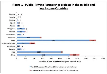
place around the world. Figure 1 depicts the PPP projects undertaken in different

(5)

Most of the middle-income countries show the up-rise in the investment of PPP

projects after 1991. However, after 1998 the lower-income groups of African

countries have only few PPP projects.

Source: Author’s own compilation from Private participation in Infrastructure Database, World Bank.

In Figure 1 we observe that number of PPP projects undertaken by Brazil, China,

India, Russia are quite high. There is a contract between private firm and the

government stating that in the contract period the revenue from the project will be

earned by the private firm and the management responsibility will also lie with them.

Usually, the contract period is in the range of 10-50 or more number of years after

which the ownership is transferred from the private firm to the government. In the

figure above, the number of PPP projects under the category of more than 50%

investment by private firms is quite high and numbers of PPP projects under the

category of less than 50% investment by the private firms are few. The World Bank in

its PPI (Private Participation in Infrastructure) Annual Report 2017 reported China

[image:5.595.89.505.152.442.2]

(6)

billion) and Pakistan (4 projects worth US dollar 5.9 billion) among the top 5 PPI

investment countries. The World Bank’s PPI Annual Report 2018 again reported

China to be the leader in PPP projects with 37 projects worth US dollar 11.6 billion.

Also, India (24 projects worth US dollar 3.8 billion) and Brazil (11 projects worth US

dollar 3 billion) were featured among the top 5 PPI investment countries in 2018. The

World Bank PPI Report noted that SAR (India, Pakistan) and ECA (Kazakhstan,

Russian Federation, Turkey) countries have a sizable portion of public debt financing

with 27% and 26% respectively.

There exists small literature dealing with a comparative evaluation of different mode

of provisioning infrastructure. Chatterjee and Morshed (2011) compare the impact of

private and government provision of infrastructure on an economy's aggregate

performance. Barro and Sala-i-Martin (1992), Futagami et. al. (1993), Fisher and

Turnovsky (1998), Devarajan et. al. (1998) study the interaction between public and

private capital in an endogenous growth context, where the public good is

non-excludable. However, excludability feature of the public good is ignored in the above

studies. A study by Ott and Tunovsky (2006) make a comparative study of the

non-excludable and an non-excludable public good. Government is the unique supplier of

public input and sets monopoly pricing of the user fees. According to them, tax plus

user fees alone could be sufficient to finance for the provision of the entire

infrastructure. However, this kind of financing is possible only in the case of

developed nations like the United Kingdom, the United States and EU nations but for

developing nations like India, only user fee cannot alone suffice the financing of the

excludable public good. Privately provided roads, power, water, transportation,

communication and irrigation etc; are quite common in the developed nations.

(7)

government fails to attract private investments. So, the governments of these countries

must use the policy instruments such as subsidy, tax holiday and sharing of partial

cost of manufacturing public good which is called Viability Gap Funding (VGF); for

example in India, the government under the VGF bears 20% - 40% of the

manufacturing cost of the infrastructure investment. Therefore, VGF could be an

important policy tool for infrastructure provision in developing nations.

In this paper, we attempt to address primarily two questions: why should the

government go for PPP for infrastructure provision? And how should the government

finance the cost of infrastructure production - through imposition of tax, through bond

financing or though charging only user-fees? We build a closed economy model of

infrastructure provision to answer these questions. In this model, infrastructure may

be provided by the pure private firm, pure public entity or through the partnership of

private firm and public entity (PPP). We are considering different possibilities: the

government may run balanced budget or may have budget deficit. In case of budget

deficit there are two possibilities: government may have constant debtor or may

accumulate debt over time. In the real world, the government borrows from the capital

market, banks and issues public bonds to finance the subsidy and public investments.

Following, Greiner (2008, 2012) and Kamaiguchi and Tamai (2012), we assume that

the government may run a deficit but it must set the primary surplus, such that it is a

positive linear function of public debt, which guarantees that the public debt is

sustainable. Greiner (2008), studies the public investment in three different situations:

the first being, the balanced budget situation, second being the situation when public

debt grows at the lesser rate than the public capital and consumption and at last the

situation when public debt grows at the same rate as capital and consumption.

(8)

mode of provision like the public and private provision has not been studied. Bara and

Chakraborty (2019), study the optimality of PPP in an endogenous growth model,

where public capital and private capital are treated as substitute and complementary

goods. However, in their paper only balanced budget case is considered and debt-

financing situation is not studied. Present paper attempts to find whether the PPP

mode under the varying budgetary regime for infrastructure provision is growth

maximizing or not, as compared to the public provision and private provision. We

find the impact of the fiscal policy in different budgetary regime: (a) when public debt

is constant, (b) When public debt is zero, (c) When public debt is accumulating. In

present paper, we find that there exists a unique steady state balanced growth rate

under all the different kinds of provision and regimes. We also find that the user fees

and growth rates are the same for the constant public debt and zero public debt under

both pure public provision and PPP provision. However, the growth rate is found to

be different for the permanent deficit under both the provision. Also, the user fee is

less under the PPP provision as compared to private provision and public provision

under certain conditions.

The structure of the paper is organized in the following manner. Section 2 describes

the competitive economy model of pure private infrastructure provision where the

behavior of firms and the representative household are studied. Section 3 describes

the model of pure public provision. Followed by section 4, which describes the

public-private partnership provision of infrastructure where both the private firm and

the government play the role in the provision of infrastructure. Section 3 and 4 also

study the steady state balanced growth rates for the constant debt case and the

permanent deficit case. Section 5 deals with the explanation of valid reasons

(9)

of debt financing or accumulating debt regime for the provision of infrastructure.

Lastly, the concluding remarks are made in section 7.

2. Pure private provision of infrastructure:

In a competitive economy closed model, we have three agents namely, the

representative household, two aggregative firms. In the pure private provision of

infrastructure the private firm sponsors the manufacturing of infrastructure for the

commercial use. The government does not play any role in the provision of

infrastructure; therefore the cost of production to the infrastructure-manufacturing

firm is unity.

2.1 Firms:

There are 2 profit-making firms in the economy. Firm 1 produces final goods for

consumption and capital accumulation. Firm 2 produces the infrastructure services.

Following Barro (1990), we assume that infrastructure services are flow in nature.

Both the firms are run by profit-maximizing private entities. Infrastructure is used for

final good production.

The household supplies physical capital required for the production of both final

goods (Y) and infrastructure (G). The production function of final goods is given as,

_,₍₁₎

is used for consumption as well as capital accumulation. denotes part of private

capital used to produce . Flow of infrastructure good at time t is denoted by . A is

the technology parameter for production of . and are output elasticities with

respect to and respectively. Final good is assumed to be a numeraire

commodity. Hence, the price of is considered to be unity.

(10)

(2)

In equation (2), denotes the remaining part of private physical capital used

to produce infrastructure. is the technology parameter of infrastructure services

production, which is a constant. The infrastructure services are productive investment

and are flow in nature. We obtain the ratio of infrastructure to private physical capital

from equation (2),

(3)

The profit function of firm 1 is given by,

₍₄₎

is the user fees or price paid by firm 1 for using infrastructure services.

The profit function of firm 2 producing flow of infrastructure service is given by,

₍₅₎

In equation (5), is the total price charged by firm 2 for providing infrastructure

services (e.g. revenue earned by selling tickets of metro rail, user fees for the usage of

roads, etc).

Substituting the value of in equation (5), we rewrite the equation as,

₍₆₎

Both firms take input prices as given and choose input quantities so as to maximize

their profit. Differentiating with respect to and , the first order condition

gives,

(7)

₍₈₎

(11)

(9)

₍₁₀₎

Differentiating with respect to , the first order condition gives,

(11)

Equating the rate of interest of firm 1 and firm 2, we find the value of ,

(12)

Now again substituting the value of in equation (10), the user fees under the private

provision is given as,

₍₁₃₎

2.2 The Households:

For the manufacturing of infrastructure the households provides the private physical

capital. The rate of accumulation of private physical capital is given by,

(14)

The rate of growth of private physical capital is,

(15)

It is assumed that the household derives utility from direct consumption of final good.

The utility function of the representative household is given by,

₍₁₆₎

is constant and denotes positive discount rate at which future utility is discounted. It

is assumed that the disposable income over expenditure is accumulated as wealth. The

total wealth/ asset (W) of the household is equal to the total private physical capital

(K) in the economy. Therefore, .

In competitive economy, the representative household maximizes the current-value

(12)

(17)

The control variable is C. The first – order maximization conditions are given as

follows:

(18)

Time derivative of the co-state variable is given by the following equation,

(19)

Taking the log and derivative of equation (18), we get,

(20)

The growth rate equation is,

(21)

2.3 Steady State Balanced growth:

At steady state balanced growth rate under the private provision, . If is

constant, is also constant. The steady state growth rate, is constant and positive.

Now setting , we get,

(22)

Therefore, the growth rate equation after substituting the value of from equation

(11) is,

(23)

Now we substitute the value of user fees from equation (13), the growth rate under the

private provision of infrastructure is,

₍₂₄₎

Proposition 1: There exists an unique steady state balanced growth rate and an user

(13)

3. Pure public provision of infrastructure:

In the pure public provision of infrastructure the government provides the

infrastructure services without the help of private firm. Therefore in a closed economy

model, we have three agents namely; the representative household, firm producing

finished goods and the government. Since, the infrastructure is fully sponsored by the

government, therefore the share of the manufacturing cost of production of

infrastructure to the government is unity. We also assume that government charges

user fees for the usage of infrastructure to the firms. Also, the government charges

capital income tax for the financing of infrastructure.

3.1 Firm:

Firm 1 is a profit-making firm, which produces the final goods for consumption and

capital accumulation. The benevolent government provides the infrastructure services.

Following Barro (1990), we assume that infrastructure services are flow in nature.

Infrastructure is used for final good production.

_,₍₂₅₎

capital used to produce . Flow of infrastructure good at time t is denoted by . A is

the technology parameter for the production of . and are output elasticities

with respect to and respectively. Final good is assumed to be a numeraire

commodity. Hence, the price of is considered to be unity.

The production function of the infrastructure provided by the benevolent government

is given by,

(14)

The ratio of infrastructure to private physical capital is given by,

(27)

₍₂₈₎

Differentiating the profit function with respect to and , the first-order

condition gives,

(29)

₍₃₀₎

Substituting the value of in the above equations,

(31)

₍₃₂₎

Infrastructure demand of firm 1 is obtained from equation (30),

(33)

Now using equations (26) and (33), the supply of infrastructure is equated with the

demand for infrastructure for finding the equilibrium quantity of private physical

capital.

(34)

Substituting the value of in the equation (31), the rate of interest is given as,

(35)

(15)

In a closed economy under the pure public provision of infrastructure the government

is mainly engaged in 3 activities: (1) It provides the infrastructure and charges user

fees for the usage of infrastructure. (2) It imposes capital income tax in order to

finance its cost. (3) It also issues government bonds. Therefore, interest on the bond

adds to the debt burden of the government while tax revenue reduces the government

debt.

The bond accumulation function is given by,

(36)

is the tax revenue at time t and is the public expenditure at time t. shows

the public investment to tax revenue. It indicates how much of it is used for the debt

service.

(37)

(38)

Substituting the value of T and E in equation (36), the bond accumulation function is

given as,

(39)

Substituting the value of from equation (26) in the above equation,

(40)

The rate of growth of bond is given as,

(41)

(16)

wealth/asset of the household denoted by W is defined as the sum of bond holding

and capital holding . Therefore,

(43)

Total disposable wealth of a household over consumption expenditure and payment

for using infrastructure services is accumulated as wealth. The rate of accumulation of

wealth is given by,

(44)

is the tax on capital income , is the interest rate, is consumption at time t.

In the economy, the representative household maximizes the current-value

Hamiltonian, subject to equation (44),

(45)

follows:

(46)

Time derivative of the co-state variable is given by the following,

(47)

(48)

Also using equation (43), we have,

(49)

(17)

(50)

Therefore, combining equations (48) and (50), the growth rate equation is obtained as,

(51)

The steady state balanced growth equilibrium is defined as a situation when

consumption, private physical capital and infrastructure capital grow at the same

strictly positive constant growth rate, i.e; . Where is positive

and constant. If is constant, then is also constant. Setting , we get the value

of as,

(52)

3.5 Steady State Balanced growth rate under the pure public provision at Zero

Debt regime:

At steady state balanced growth rate under the pure public provision, the government

doesn’t have any debt such that the government’s tax revenue is equal to the total

expenditure of the government. In other words, the government observes the balanced

budget. Setting , we have,

(53)

Substituting the value of in the above equation we have,

(54)

Now again substituting the value of and in the above equation, we get the value of

under the pure public provision zero-debt regime,

(55)

(18)

The growth rate is given as,

(56)

Substituting the value of in the above equation, we have,

(57)

Now substituting the value of user fees under the pure public provision zero-debt

case,

(58)

3.5.2 Growth maximizing tax rate under the pure public provision at zero debt

or balanced budget regime:

Differentiating the growth rate equation (58) with respect to , the first-order

condition is,

(59)

Therefore, equation (59) implies the growth maximizing tax rate is zero.

3.5.3 Maximum growth rate:

Substituting the growth maximizing tax rate in the growth rate equation (58), we get

the maximum growth rate under the balanced budget for the pure public provision,

(60)

Proposition 2: The growth maximizing tax rate under pure public provision of

infrastructure is zero. It is optimal for the government to charge user fees instead of

imposing tax for financing infrastructure. And, the maximum growth rate under the

balanced budget for the pure public provision of infrastructure is equal to the

(19)

3.6 Steady State Balanced growth rate under the pure public provision at

constant Debt regime:

At steady state balanced growth rate, the government experiences the constant debt,

such that and also is constant and positive. However, when

, it does not necessarily imply that public debt equals zero. If the level of initial

debt is positive, the debt to capital ratio and also the debt to GDP ratio are positive but

decline over time and converge to zero in the long run.

Therefore, setting , we find that the user fees under the pure public provision at

constant debt regime is same as under the pure public provision at zero debt regime.

Therefore the growth rate and growth maximizing tax rate are also same. Equation

(61)-(64) of Appendix A1 show that the user fees, growth rate, growth maximizing

tax rate, and the maximum growth rate respectively, under the balanced budget for the

pure public provision at constant debt regime, which are exactly same as the balanced

budget regime.

Proposition 3: For the public provision of infrastructure, the user fee charged for

infrastructure services and growth rates under the constant debt regime and the

balanced budget (zero debt) regime are the same.

3.7 Steady state balanced growth rate under the pure public provision at

permanent deficit or accumulating debt regime:

At steady state balanced growth rate, the government experiences the case when debt

is accumulating; this is the case of a permanent deficit. Steady state balanced growth

rate is positive and constant and therefore, all the variables grow at the same strictly

(20)

is characterized by the public deficits, where the government debt grows at the same

rate as all other endogenous variables in the long run.

For the sustainability of public debt in our model, we apply the primary surplus rule,

which states that the primary surplus relative to GDP is a function that positively

depends on the debt to GDP ratio. According to Greiner (2013), ‘the economic

rationale behind the rule is to make the debt ratio a mean-reverting process when the

reaction of the primary surplus is sufficiently large, preventing the debt to GDP ratio

from exploding’. There are also empirical evidences revealing that the governments

follow such a rule of primary surplus. For example, Bohn (1998) and Greiner et al.

(2007) have shown that this rule holds for the USA and for selected European

countries, respectively, using OLS estimations. Also Fincke and Greiner (2012) find

that the reaction coefficient determining the response of the primary surplus to public

debt is not a constant but time varying with the average of that coefficient being

strictly positive for some euro area countries. The model by Barro (1990), has been

extended by Kamaiguchi and Tamai (2012) by integrating public deficit and public

debt into the model to analyze the conditions for simultaneous growth and

sustainability of public debt.

Therefore, following Greiner (2008) and Kamaiguchi and Tamai (2012), we assume

that the ratio of the primary surplus to gross domestic income ratio is a positive linear

function of the debt to gross domestic income ratio with an intercept. Hence, the

primary surplus ratio can be written as,

(65)

‘Where are the real numbers and are constant. determines how strongly the

primary surplus reacts to changes in public debt. determines whether the level of the

(21)

implies that primary surplus declines as GDP rises and the government increases

it’s spending with higher GDP. In this case of negative , must be sufficiently large.

If is sufficiently low, then the government must be a creditor for the economy to

achieve sustained growth. If > 0 implies that primary surplus rises as GDP

increases. In this case, must not be too large. A high implies that government

does not invest sufficiently and he must be a creditor in order to finance its

investment, in order to achieve sustained growth.’ (Greiner, 2008)

From equation (65),

(66)

Substituting the values of , and in the above equation, we get another value of

under the permanent deficit case, which is different from the balanced budget ,

therefore,

–

(67)

The bond accumulation function for the sustainability of public debt is,

(68)

After substituting the value of in the above equation, the rate of growth of bond is,

(69)

Now substituting the value of and in the above equation, the rate of growth of

bond under the pure public provision at accumulating debt regime is given as,

(70)

Resorting to equation (51) and (70), we set , we obtain the value of user fees

under the pure public provision at accumulating debt regime.

(22)

3.7.1 Growth rate under the pure public provision at accumulating debt or

permanent deficit regime:

Substituting the value of user fees under the pure public provision at accumulating

debt regime, we obtain the growth rate equation as,

(72)

3.7.2 Growth maximizing tax rate under the pure public provision at

accumulating debt regime:

We differentiate the growth rate equation (72) with respect to . Therefore, the first

order condition gives the value of optimal tax rate under the pure public provision at

accumulating debt regime,

(73)

From the second order condition, we have,

(74)

Therefore,

is a sufficient condition for .

3.7.3 Maximum growth rate under the pure public provision at accumulating

debt regime:

Substituting the value of growth maximizing tax rate under the pure public provision

at accumulating debt regime in the growth rate equation (72), we obtain the maximum

growth rate as,

+

(23)

Proposition 4: The user fees and maximum growth rates under the pure public

provision at accumulating debt regime are different from the user fees and maximum

growth rates under the public provision at constant debt and balanced budget regime.

4. Public-Private Partnership provision of infrastructure:

In the Public-Private Partnership provision of infrastructure the government provides

the infrastructure services with the help of private firm. However, in the partnership

venture the ownership lies with the private firm and the government makes a small

partial investment for manufacturing. In real life there are number of PPP contracts

such as Operate-Transfer (BOT), Own-Operate-Transfer (BOOT),

Build-Own-Operate-Transfer (BOOT), Build-Finance-Operate (DBFO),

Design-Construct-maintain-Finance (DCMF) etc. The private firm transfers the ownership to

the government in 10-50 years or more time period after making its profit revenues

from the user fees. In countries, where PPP projects are implemented, there is VGF

(Viability Gap Funding) through which government makes a direct investment up to a

certain percentage (say, 20% in case of India) of the total cost to the

infrastructure-producing firm. The government, if it so decides may provide additional grants out of

its budget up to further 20% of the total project cost. VGF is in the form of a capital

grant to the infrastructure-manufacturing firm for the construction of the

infrastructure project.

In our model, we construct a model where the government makes the partial

investment in the private firm. Therefore, following the real life examples of viability

gap funding, it is assumed that the government bears fraction of total cost of

manufacturing infrastructure . The model is a competitive economy closed

(24)

firms and the government. Firm 1 produces the finished goods and firm 2

manufactures the infrastructure. The government invests in firm 2 not only because of

the positive externality derived from the infrastructure but also because infrastructure

is essential for final good production and welfare enhancement. First we look at the

manufacturing sector, followed by the government sector and then the household

sector.

4.1 Firms:

Firm 1 produces final goods for consumption and capital accumulation. Firm 2

provides the infrastructure services and charges user fees for it. Following Barro

(1990), we assume that infrastructure services are flow in nature. Both the firms are

run by profit maximizing private entities. Infrastructure is used for final good

production.

_,₍₇₆₎

capital used to produce . Flow of infrastructure good at time t is denoted by .A is

the technology parameter for production of . and are output elasticities with

respect to and respectively. Final good is assumed to be a numeraire commodity.

Hence, the price of is considered to be unity.

The production function of infrastructure service is given as,

(77)

In equation (77), denotes the remaining part of private physical capital used

to produce infrastructure. is the technology parameter of infrastructure services

(25)

and are flow in nature. We obtain the ratio of infrastructure to private physical capital

from equation (77),

(78)

₍₇₉₎

The profit function of firm 2 producing flow of infrastructure service is given by,

₍₈₀₎

In equation (80), is the total price charged by firm 2 for providing infrastructure

services (e.g. revenue earned by selling tickets of metro rail, user fees for the usage of

roads, etc) and is the share of cost borne by firm 2 for manufacturing infrastructure.

Substituting the value of from equation (77) in the above equation, we have,

₍₈₁₎

Both firms take input prices as given and choose input quantities so as to maximize

their profit. Differentiating with respect to and , the first order condition

gives,

(82)

₍₈₃₎

Substituting the value of in the above equations,

(84)

₍₈₅₎

Infrastructure demand of firm 1 is obtained from equation (83),

(26)

Now using equations (77) and (86), the supply of infrastructure is equated with the

demand for infrastructure for finding the equilibrium quantity of private physical

capital.

(87)

Substituting the value of in the equation (84), the rate of interest under the public

provision is given as,

(88)

4.2 The Government:

In the decentralized economy under the public-private partnership provision of

infrastructure the government is mainly engaged in 3 activities: (1) It bears the partial

cost burden of manufacturing infrastructure. (2) It imposes capital income tax in order

to finance its cost. (3) It also issues government bonds.

The government in this economy receives fund by imposing income tax and by

issuing government bonds. The interest on the bond and expenditure incurred for

sharing of cost of producing infrastructure service and subsidizing its production add

to the debt burden of the government while tax revenue reduces the government debt.

Hence the bond accumulation function is given by,

(89)

is the tax revenue at time t and is the public expenditure at time t. shows

the public investment to tax revenue. It indicates how much of it is used for the debt

service.

(90)

(27)

in the above equation represents the share of cost of manufacturing

infrastructure, borne by the government.

Substituting the value of T and E in equation (89), the bond accumulation function is

given as,

(92)

The rate of growth of bond is given as,

(93)

₍₉₄₎

wealth/asset of the household denoted by W is defined as the sum of bond holding

and capital holding . Therefore,

(95)

Total disposable wealth of a household over consumption expenditure and payment

for using infrastructure services is accumulated as wealth. The rate of accumulation of

wealth is given by,

(96)

is the tax on capital income , is the interest rate, is consumption at time t.

In competitive economy, the representative household maximizes the current-value

Hamiltonian, subject to equation (96),

(28)

follows:

(98)

Time derivative of the co-state variable is given by the following,

(99)

(100)

Also using equation (95), we have,

(101)

Since , now substituting these values in the above equation, we get,

(102)

Therefore, combining equations (100) and (102), the growth rate equation is obtained

as,

(103)

The steady state balanced growth equilibrium is defined as a situation when

consumption, private physical capital and infrastructure capital grow at the same

strictly positive constant growth rate, i.e; . Where is positive

and constant. If is constant, then is also constant. Setting , we get the value

of as,

(29)

4.5 Steady State Balanced growth rate under the PPP provision at Zero Debt

regime:

At steady state balanced growth rate under the PPP provision, the government doesn’t

have any debt such that the government’s tax revenue is equal to the total expenditure

of the government. In other words, the government observes the balanced budget.

Setting , we have,

(105)

Substituting the value of in the above equation, we get the value of under the PPP

provision at zero-debt regime,

(106)

4.5.1 Growth rate under the PPP provision at zero debt regime:

The growth rate is given as,

(107)

Now substituting the value of user fees of the PPP at zero-debt regime the growth rate

equation is,

(108)

4.5.2 Growth maximizing tax rate under the PPP provision at zero debt regime:

To find the growth maximizing tax rate, we do the logarithmic transformation of

growth rate equation (108),

(109)

Differentiating the log-transformed growth rate equation with respect to , the first

order condition gives,

(110)

(30)

(111)

The second order condition gives,

(112)

is a sufficient condition for the growth maximizing tax rate under the PPP

provision at zero debt regime.

Proposition 5: At balanced budget and constant debt regime, for the public provision

the growth maximizing tax rate is zero, but for the PPP provision the growth

maximizing tax should be less than 50%.

4.6 Steady State Balanced growth rate under the PPP provision at constant Debt

regime:

At steady state balanced growth rate, the government experiences the constant debt,

such that and also is constant and positive. However, when

, it does not necessarily imply that public debt equals zero. If the level of initial

debt is positive, the debt to capital ratio and also the debt to GDP ratio are positive but

decline over time and converge to zero in the long run.

Therefore, setting , we find that the user fees under the PPP provision at

constant debt regime is same as under the PPP provision at zero debt regime.

Therefore the growth rate and growth maximizing tax rate are also same.

Equation (113)-(116) of Appendix A2 shows the user fees, growth rate, growth

maximizing tax rate, and maximum growth rate respectively for the PPP provision at

the constant debt regime, which are exactly same as the balanced budget regime.

Proposition 6:For the PPP provision, the user fee charged for infrastructure services

and growth rates under the constant debt regime and the balanced budget regime are

(31)

4.7 Steady state balanced growth rate under the PPP provision at permanent

deficit regime:

At steady state balanced growth rate, the government experiences the case when debt

is accumulating; this is the case of a permanent deficit. Steady state balanced growth

rate is positive and constant and therefore, all the variables grow at the same strictly

positive constant rate, such that .The permanent deficit case

is characterized by the public deficits, where the government debt grows at the same

rate as all other endogenous variables in the long run.

Applying the primary surplus rule, we get

(117)

Substituting the values of , and in the above equation, we get another value of

under the permanent deficit case, which is different from the balanced budget ,

therefore,

–

(118)

The bond accumulation function for the sustainability of public debt is,

(119)

After substituting the value of in the above equation, the rate of growth of bond is,

(120)

Now substituting the value of and in the above equation, the rate of growth of

bond under the PPP provision at permanent deficit regime is given as,

(32)

Resorting to equation (103) and (121), we set , we obtain the value of user fees

under the PPP provision at permanent deficit regime.

– (122)

4.7.1 Growth rate under the PPP provision at constant debt regime:

Substituting the value of user fees under the PPP provision at permanent deficit

regime, we obtain the growth rate equation as,

(123)

4.7.2 Growth maximizing tax rate under the PPP provision at permanent deficit

regime:

We differentiate the growth rate equation with respect to . Therefore, the first order

condition gives the value of optimal tax rate under the PPP provision at permanent

deficit regime,

(124)

From the second order condition, we have,

(125)

Therefore,

is a sufficient condition for .

4.7.3 Maximum growth rate under the PPP provision at accumulating debt

regime:

Substituting the value of optimal tax rate for the PPP provision under the

accumulating debt regime, we get the maximum growth rate equation as,

(33)

Proposition 7: The user fees and maximum growth rates under the PPP provision at

accumulating debt regime are different from the user fees and maximum growth rates

under the PPP provision at constant debt and balanced budget regime.

5. Justification of Public-private partnership provision of infrastructure:

We need to know whether the growth rates or rather the maximum growth rates for

which provision is better and could be suggested for policy prescription. For that

matter we make a comparison of the PPP mode with the private / public mode.

Therefore, comparing the maximum growth rates under the PPP provision at balanced

budget or constant debt and the maximum growth rates under the public / private

provision at balanced budget or constant debt, we find that,

(127)

Therefore the Public-Private Partnership is justified under the condition, if

. In other words, as the share of manufacturing cost of

infrastructure borne by the government is low, PPP provision of infrastructure yields

higher growth rate.

Suppose,

. Taking the logarithmic transformation of . We obtain the

equation,

(128)

Differentiating above equation with respect to ,

(34)

From equation (129), is a sufficient condition for

to be positive. It

follows that when output elasticity from the infrastructure capital is more than 0.5,

then with increase in , there is higher chance that the condition (A) is satisfied

justifying the adoption of the Public-Private Partnership (PPP) provision of

infrastructure. Hence, the countries whose output elasticity from the infrastructure

capital is sufficiently high should go for the PPP mode for the provision of

infrastructure.

Proposition 8: In zero debt case, if the output elasticity from the infrastructure

capital should be sufficiently high and share of manufacturing cost of infrastructure

borne by the government is low, PPP provision of infrastructure yield higher growth

rate compared to pure public or pure private provision of infrastructure.

Also comparing the user fees under the private provision and public provision (at both

accumulating debt and balanced budget/constant debt case) with the PPP provision (at

both accumulating debt and balanced budget / constant debt case), we have the

following results:

(130)

From equation (130) it follows that, when

, user fee charged under

pure private provision of infrastructure is higher than that under PPP. In PPP, if

growth maximizing tax rate is imposed, the above condition reduces to .

Thus, if the share of manufacturing cost borne by the private firm is low in PPP,

user-fee charged under private provision is higher than that under PPP in zero debt case,

(35)

This justifies PPP from the consumer’s utility perspective as well and therefore, the

government could opt for the PPP provision if the output elasticity for the

infrastructure capital increases due to VGF financing by the government.

Proposition 9: If the share of cost borne by the government for infrastructure

provision is high, then user fee charged under PPP would be lower, which

may give another reason to justify PPP.

6. Justification for debt financing:

Another question is that why should government go for the debt financing and not the

balanced budget or constant debt. In order to show the necessity of debt financing

we make a comparison between the maximum growth under the PPP mode at

accumulating debt regime with that of the maximum growth rate under the PPP mode

at constant debt or zero debt regimes. We find that,

(131)

From equation (131), it follows that when

then debt financing

under the PPP mode of provision is feasible.

Proposition 10: For technologically poor countries or less developed countries, debt

financing is desirable.

7. Conclusion:

This paper explains when the PPP mode of infrastructure provision is desirable in a

model with non-rival yet excludable infrastructure in a closed economy model. The

model shows that if output elasticity of infrastructure is sufficiently high and share of

manufacturing cost borne by the government is low, PPP provision of infrastructure

(36)

charging lower user fees as well. PPP provision may be justified on that ground too.

The model also shows that for the technologically poor countries debt financing may

be desirable.

There is a vast literature that deals with financing problem of public good through

pure public provision of infrastructure. But, there is not a single paper on endogenous

growth theory, which deals with the financing problem of public good through PPP.

This paper tries to answer the two questions: (1) why should the government go for

the PPP for the infrastructure provision? (2) How should the government finance the

cost of infrastructure production – (a) through imposition of tax (b) through bond

financing and (c) through charging user fees? We find the conditions under which the

maximum growth rate under the PPP mode of provision is greater than the private and

public provision. Also, the user fees and growth maximizing tax rates under different

regimes have been found out. User-fee under the PPP mode is less as compared to the

pure private user fees and pure public user fees, due to VGF investment by the

government, which keeps the PPP user fees lower. We also find that in zero debt case,

for pure public provision of infrastructure, charging user fees is better than the

imposition of tax. This paper also explains why in some nations there are huge

number of PPP investments and why in some nations we find only few PPP projects.

The nations where, the output elasticity from the infrastructure is very high say, more

than 50%, there only the PPP projects yield higher growth rates.

However, like any other theoretical model, this model also has few limitations. This

model does not contain many aspects of the reality - like the imperfect competition in

the production of infrastructure, infrastructure as a stock variable etc. In our future

research we aspire to find optimal fiscal policy by taking these aspects into the

(37)

incorporate the public private partnership in infrastructure provision in endogenous

growth model with constant, zero and accumulating government debt.

APPENDIX

Appendix A1. For the pure public provision under the constant debt, .

Therefore, from equation (36), we have,

Hence,

Substituting the value of and in the above equation, we have,

Substituting the value of , we get,

Since converges to zero in the long run, therefore from the above equation we have,

By simplifying the above equation we obtain the value of for the constant debt

regime.

(61)

Now substituting the value of user fees under the pure public provision constant-debt

regime,

(62)

(38)

(63)

Since the first-order condition is negative for the pure public provision under constant

debt, the growth maximizing tax rate is zero.

Now the maximum growth for the pure public provision under the constant debt

regime is equal to the private provision growth rate.

₍₆₄₎

Appendix A2. For the PPP provision under the constant debt, . Therefore, from

equation (88), we have,

Hence,

Substituting the value of and in the above equation, we have,

From above equation,

Since converges to zero in the long run, therefore from the above equation we have,

Substituting the value of in the above equation, we obtain the value of user fees for

the infrastructure services under the PPP provision for the constant debt regime.

(113)

Now substituting the value of user fees under the PPP provision constant-debt regime,

(114)

To find the growth maximizing tax rate, we do the logarithmic transformation of

equation (113),

Differentiating the log-transformed growth rate equation with respect to , the first-

order condition gives,

The optimal tax rate under the PPP provision at constant debt regime is,

(115)

(39)

is a sufficient condition for the growth maximizing tax rate under the PPP provision at constant debt regime.

Substituting the value of optimal tax rate under the PPP provision at constant debt

regime, we get the maximum growth rate,

(116)

Now the maximum growth for the PPP provision under the constant debt regime is

equal to the PPP provision under the balanced budget regime.

References:

Barro, R.J., 1990. Government Spending in a Simple Model of Endogenous Growth.

Journal of Political economy, 98, S103-S125.

Barro, R.J., Sala-i-Martin, X., 1992. Public Finance in Models of Economic Growth.

The Review of Economic Studies,59,645-661.

Bara, A.A., Chakraborty, B., 2019. Is Public-Private Partnership an Optimal Mode of Provision of Infrastructure? Journal of Economic Development, Vol. 44, No.1.

Bohn, H., 1998. The Behaviour of U.S Public Debt and Deficits. Quarterly Journal of Economics, volume 113, Issue 3, 949-963.

Bhattacharya, C., 2014.A Note on Endogenous Growth with Public Capital. Munich Personal RePEc Archive, MPRA paper No. 55728, online at http://mpra.ub.uni_muenchen.de/55728/

Chatterjee, S., Morshed, A.K.M.M., 2011. Reprint to: Infrastructure Provision and Macroeconomic Performance. Journal of Economic Dynamics and Control, 35, 1405-1423.

Dasgupta, D., 1999.Growth versus Welfare in a Model of Nonrival Infrastructure.

Journal of Development Economics, Vol. 58, 359-385.

Devarajan, S., Xie, D.,Zou H., 1998. Should Public Capital be Subsidized or Provided? Journal of Monetary Economics, 41, 319-331.

Fincke, B., Greiner, A., 2012. How to Assess Debt Sustainability? Some Theory and Empirical Evidence for Selected Euro Area Countries. Applied Economics, Vol. 44, Issue 28, 3717-3724.

(40)

Futagami, K., Morita, Y., Shibata, A.,1993. Dynamic analysis of an endogenous growth model with public capital. The Scandinavian Journal of Economics, volume 95, No. 4, 607-625.

Greiner, A., Koller, U., Semmler, W., 2007. Debt sustainability in the European Monetary Union: Theory and empirical evidence for Selected Countries. Oxford Economic Papers, New Series, volume 59, 194-218. Oxford Journals, Oxford University Press.

Greiner, A.,2008. Human Capital Formation, Public Debt and Economic Growth.

Journal of Macroeconomics, 30, 415-427.

Greiner, A., 2008. Does it pay to have a Balanced Government Budget? Journal of Institutional and Theoretical Economics (JITE).Vol. 164, No. 3, 460-476.

Greiner, A., 2012. Public Capital, Sustainable Debt and Endogenous Growth.

Research in Economics, 66, 230-238.

Greiner, A., 2013. Public Debt, Productive Public Spending and Endogenous Growth.

Working Papers in Economics and Management, Bielefeld University, No-23-2013.

Kamiguchi, A., and Tamai, T., 2012.Are Fiscal Sustainability and Stable Balanced Growth Equilibrium Simultaneously Attainable? Metroeconomica International Review of Economics, 63:3, 443-457.

Kateja, A., 2012. Building Infrastructure: Private Participation in Emerging Economies. International Conference on Emerging Economies – Prospects and Challenges (ICEE-2012). Procedia - Social and Behavioural Sciences, 37, 368-378.

Tsoukis, C., and Miller, N. J., 2003. Public Services and Endogenous Growth.

Journal of Policy Modeling, 25, 297-307.