Munich Personal RePEc Archive
Inference for likelihood-based estimators
of generalized long-memory processes
Beaumont, Paul and Smallwood, Aaron
Florida State University, University of Texas-Arlington
30 September 2019
Online at
https://mpra.ub.uni-muenchen.de/96313/
Inference for likelihood-based estimators of generalized
long-memory processes
✩Paul M. Beaumonta, Aaron D. Smallwoodb,∗
a
Department of Economics, Florida State University, Tallahassee, FL 32306, USA b
Department of Economics, University of Texas Arlington, 701 S. West Street. (mailbox: 19479), Arlington, TX 76019, USA
Abstract
Despite a recent proliferation of research using cyclical long memory, surprisingly little is known regarding the asymptotic properties of likelihood-based methods. Estimators have been studied in both the time and frequency domains for the Gegenbauer autoregressive moving average process (GARMA). However, a full set of asymptotic results for all parameters has only been proposed by Chung
(1996a,b), who present somewhat tenuous results without an initial consistency proof. In this paper, we review the GARMA process and the properties of fre-quency and time domain likelihood-based estimators using Monte Carlo analysis. The results demonstrate the strong efficacy of both estimators and generally sup-port the proposed theory of Chung for the parameter governing the cycle length. Important caveats await. The results show that asymptotic confidence bands can be unreliable in very small samples under weak long memory, and the distribution theory under the null of an infinitely long cycle appears to be unusable. Possible solutions are proposed, including the use of narrower confidence bands and the application of theory under the alternative of finite cycles.
Keywords: long memory, GARMA, CSS estimator, Whittle estimator
JEL Classification Codes: C22, C40, C58, G12
✩The authors acknowledge the Texas Advanced Computing Center (TACC) at The University
of Texas at Austin for providing HPC resources that were used to generate simulation results in the paper. URL: http://www.tacc.utexas.edu.
∗Corresponding author: Aaron D. Smallwood, Department of Economics, University of Texas
Arlington, 701 S. West Street (mailbox: 19479), Arlington, TX 76019, USA
Email addresses: [email protected](Paul M. Beaumont),[email protected](Aaron D.
1. Introduction
Few contributions to time series analysis have fomented more interest than the introduction of long memory by Granger and Joyeux (1980) and Hosking
(1981). These methods allow for slowly decaying autocorrelation functions and the existence of spectral density functions with one or more singularity. In eco-nomics, long memory has provided a major breakthrough in allowing researchers to bridge the gap between unit roots and transitory I(0) dynamics.
As emphasized by Dissanayake et al. (2018), attention has recently focused on methods that can accommodate cyclical long memory, including seasonal long memory and Gegenbauer autoregressive moving average (GARMA) models. The GARMA model, which has received specific attention, is defined as follows,
(1−2ηL+L2)λφ(L)(xt−µ) =θ(L)εt (1)
whereφ(L) andθ(L) arepand q order polynomials in the lag operatorL, andεt is a mean zero disturbance sequence with E(ε2
t) =σ2 and no serial correlation. Withν= cos−1
(η) the process possesses a spectral density function given by
f(ω) = σ 2
2π
θ(e−iω
)
φ(e−iω)
2|cos(ω)−cos(ν)|−2λ
. (2)
When p = q = 0, the process has an autocorrelation function at lag j that is proportional to cos(jν)j2λ−1
. When ν = 0, the result is an ARF IM A(p,2λ, q) process as originally studied byGranger and Joyeux(1980) and Hosking(1981). The process above is covariance stationary providedλ <1/4 whenν ∈ {0, π} or whenλ <1/2 otherwise (Gray et al. 1989).
This model, and its extension, the k-factor GARMA model, have been ap-plied across virtually every discipline that uses time series methods. Examples include atmosphere C02 (Woodward et al. 1998), sunspots (Chung 1996b;Artiach and Arteche 2012), dust pollution (Reisen et al. 2014), river flow (Diongue and Ndongo 2016), electricity demand (Leschinski and Sibbertsen 2019), and traffic patterns (Ferrara and Gu´egan 2001). In economics and finance, the GARMA and k-factor GARMA models have been applied to study information related to equities (Beaumont and Smallwood 2019;Lu and Guegan 2011;Caporale and Gil-Alana 2014), interest rates (Ramachandran and Beaumont 2001;Gil-Alana 2007;
Asai et al. 2018), inflation (Arteche and Robinson 2000;Caporale and Gil-Alana 2011;Peiris and Asai 2016), and unemployment (Gil-Alana 2007).
et al. 2001) and semi-parametric estimators (Hidalgo and Soulier 2004;Hidalgo 2005) extending the log-periodogrom estimators of Geweke and Porter-Hudak
(1983) andRobinson (1995). However, a full set of accepted asymptotic results does not exist. Yajima (1996) showed that maximization of the periodogram could be used to consistently estimate the position of spectral poles, which would include ν. For semi-parametric estimators, Hidalgo and Soulier (2004) provide an asymptotic result for λ based on (1), demonstrating that the distribution for ν unknown is identical to that for ν known. Hidalgo (2005) extends these results and provides an estimator forν that is asymptotically normal with rate of convergenceTβ, withβ <1, and T denoting the sample size, whose distribution depends on whether ν = {0, π} or ν ∈ (0, π). Giraitis et al. (2001) provide the asymptotic distribution forλ for the parameterized Whittle estimator, and establish rateT convergence for the estimate of ν. Unfortunately, as discussed below,Giraitis et al.(2001) are unable to provide a full set of asymptotic results for their estimator ofν.
Obtaining valid inference forη is vital for researchers interested in obtaining confidence bands for estimated cycles and is imperative for those interested in tests for specific values, such asη= 1. Perhaps the most promising results were proposed by Chung (1996a,b) who argued that the constrained sum of squares (CSS) estimator forη converges at either rate T (if |η|<1) orT2 (if |η|= 1) to ratios of functionals of Brownian motion processes. Estimates for the remaining parameters achieve asymptotic normality at the standard rate ofT1/2
. The CSS based results have recently been extended byBeaumont and Smallwood (2019) to consider multiple long memory cycles, while Peiris and Asai (2016) provide proposed distribution results for the estimator with heteroskedastic disturbances. Regrettably, given the potential discontinuity in the distribution for η coupled with the existence of a closed parameter space for this parameter, an initial consistency proof for the CSS estimators has proven quite elusive. Specifically, Chung and related extensions rely on the observation that the score evaluated at the true parameters is zero, which, as pointed out by Giraitis et al. (2001), may not be sufficient to establish consistency. Given the concerns regarding the theoretical results for the CSS estimator, it remains an open question as to whether or not the theory is practically useful.
fatter tails and a more peaked density than theory implies. Although the problem may become negligible for very large samples, differences between theoretical and empirical densities can become severe for very small T and values of λ close to zero, such that asymptotic confidence bands can be quite unreliable. Further, the results show that the use of distribution theory under the case|η|= 1 can lead to severe size distortion potentially complicating issues for researchers attempting to test if a finite cycle exists.
Awaiting additional theoretical results, we can offer practical solutions to researchers interested in estimating confidence bands and employing statistical tests. For small estimated values ofλ, researchers should avoid using asymptotic results when the sample size is small. Otherwise, results do show that narrower asymptotic confidence bands can be quite reliable, even for moderately small samples. Thus, a recommendation is made that when using theory, multiple sets of confidence intervals should be presented. Finally, in testing the hypothesis that
|η|= 1, more conservative statistics based on the distribution theory under the alternative appear to yield more reliable results. A parametric bootstrap applied to US unemployment supports this assertion, and we can further recommend that whenever possible theoretical limitations can potentially be overcome through computational methods.
The rest of the paper is organized as follows. In Section 2, we motivate the problem using the US unemployment rate and present the two estimators of the GARMA process due to Chung (1996a,b) and Giraitis et al. (2001). In section 3, we present the Monte Carlo results, concentrating on the calculation of confidence bands. Section 4 offers evidence specific to testing|η|= 1, and a final section concludes.
2. Parametric Estimators of the GARMA Process
The two estimators analyzed here use time and frequency domain approxi-mations for the Gaussian log likelihood function based on the GARMA process defined in (1). The first estimator we consider is a Whittle type estimator. For a sample sizeT, let ˜T = [T /2], where [·] denotes the integer part. Let ∆ denote the set of all possible parameter values for δ = {φ′
, θ′
, λ, µ} and let QT denote the set of Fourier frequencies,ωj = 2π j/T. Based on the spectrumf(ωj) defined in (2), Giraitis et al.(2001) propose the following estimator (denoted GHR),
ˆ
δ
ˆ
ν
where
S(δ, ν) =
1 ˜ T T X j=0
I(ωj)
f(ωj)
and I(ωj) =
1 2πT T X t=1
xteitωj
2 . (3b)
Importantly, note that the estimate ofν is obtained with respect to the discrete set QT, and that the true value of ν need not be in this set. Under suitable regularity conditions, Giraitis et al. (2001) establish asymptotic normality for their estimate of δ, and prove that the estimate of ν is consistent. However, a limiting distribution for ˆν is not available, since the function in (3) is not minimized for all values in the interval [0, π].
Concentrating out the residual variance, and under a Gaussian assumption for εt, our second estimator is based on the constrained sum of squares (CSS) function of the parameters,φ′
, θ′
, λ, η, µand is given by
L(φ′
, θ′
, λ, η, µ) =−T
2
"
ln(2π) + ln 1
T
T
X
t=1
ε2t
!
+ 1
#
. (4)
Under an initialization assumption, maximization of the CSS function produces a set of estimates that is asymptotically equivalent to the maximum likelihood values.
The proposed theory of Chung(1996b) establishes asymptotic normality for
δ= (λ, φ′
, θ′
)′
, where, for example, the element from the information matrix forλ
is given byIλ= 2(π2/3−πν+ν2). For the CSS estimate ofη, which is found to be asymptotically independent ofδ, Chung has the following proposed distributional result in his Theorem 2:
T(ˆη−η)→
d
sin(ν)
λ Y0 =
sin(ν)
λ
R1
0 W1dW2−
R1
0 W2dW1
R1
0 W12(r)dr+
R1
0 W22(r)dr
, for|η|<1 (5)
and
T2(ˆη±1)→
d ∓ 1
2λY1 =∓
1 2λ
R1
0
Rr
0 W(s)ds
dW(r)
R1
0
Rr
0 W(s)ds
2
dr , forη=±1 (6)
whereW, W1, and W2 are independent Brownian motions. Percentiles ofY0 and
Y1 can be simulated to yield confidence bands and test statistics forη.
2019,1
(1−2∗0.9986L+L2)0.326(1−0.934L−0.026L2)(ut−6.16) = (1−0.567L)εt. (7)
With ˆη= 0.9986<1, the estimated model represents a stationary process, albeit highly persistent, with strong cycles. In contrast, ifη= 1, the model reduces to a non-stationary ARFIMA process lacking a finite cumulative impulse response function. The asymptotic 99% confidence bands constructed under the assump-tion η = 1 are [0.9980,9987], while the corresponding quantities based on rate
T convergence are [0.9972,1.0001].2 Although more formal testing procedures advocated below generally yield evidence in support ofη <1, casual observation of these confidence bands could prove confusing. The disparate conclusions also highlight one of the potential concerns as it relates to the use of the proposed distribution for the CSS estimator. In the following sections, we provide Monte Carlo analysis to shed light on the applicability of theoretical results both in forming confidence bands and for testingη= 1.
3. The Monte Carlo Results
In this section, we present Monte Carlo results to assess how the estimators perform both in small and larger samples. From a computational perspective, an advantage of the Whittle based estimator of Giraitis et al. (2001) is its relative simplicity. For each Fourier frequency,ωj, we minimize the functionS(δ, ωj) in (3) with respect toδ, and track the value of the objective function forj= 0,1, . . . ,T˜. The estimate ofν, ˆν, is the Fourier frequency associated with the minimum value of the objective function amongst the ˜T+ 1 alternatives. Then, the estimate ofδ
is the value that minimizes the objective function with the frequency fixed at ˆν. An estimate ofηcan be obtained through the functional relationship,η= cos(ν).
For the CSS estimator, note that the polynomial (1−2ηL+L2)−λ
is related to the Gegenbauer polynomials,cj, as follows (Gray et al. 1989):
(1−2ηL+L2)−λ
=
∞ X
j=0
cjLj, (8a)
1
Data are from the St. Louis Federal Reserve Bank. The GARMA(2,1) model was selected on the basis of the AIC for all combinations of models withpandqless than 2.
2
These quantities are calculated using (5) and (6) based on Chung’s simulated values for Y0 and Y1. For example, the value of the 1st and 99th percentiles for Y0 is -4.238 and
where
cj = [j/2]
X
k=0
(−1)kΓ(λ+j−k)(2η)j−2k
Γ(λ)Γ(k+ 1)Γ(j−2k+ 1) (8b)
and Γ(·) is the gamma function. Starting fromc0 = 1 andc1 = 2ηλ, the Gegen-bauer polynomials can be computed recursively as
cj = 2η
λ+ 1
j + 1
cj−1−
2λ+ 1
j + 1
cj−2. (9)
The disturbance sequence in (1) is a function of the model parameters and in turn the Gegenbauer polynomials as follows,
εt= (1−φ1L− · · · −φpLp)(xt−µ)− t−1 X
j=1
cjεt−j
−θ1 t−2 X
j=0
cjεt−j−1− · · · −θq
t−q−1 X
j=0
cjεt−j−q. (10)
To calculate the model parameters,Chung(1996a,b) andGray et al.(1989), ad-vocate a line-search forη.3 This implies that the parameter space being searched over is a discrete set. This seems especially unfortunate as the theory is developed under the assumption of a continuous parameter space and a potential advantage of the CSS estimator relative to the GHR counterpart is lost. In instances where the true value of η is unknown, a discretization implies that potentially large biases can result or that a very fine grid would need to employed. Further, if a large number of grid points is selected, it almost certainly becomes necessary to impose boundary constraints onη for computational purposes.
Here, we advocate the use of a double gradient-based procedure as in Ra-machandran and Beaumont (2001). A set of starting values for η is selected, which is typically a grid from -1 to 1, using a relatively small step size to avoid potential local minima. Conditional on each value of η in the grid, an estimate of δ is obtained using a gradient based method. Conditional on the estimate of
δ, we estimate the parameter η, again using a search algorithm. The procedure continues as we update the value of η along the grid. Once a neighborhood for the maximum value of the CSS function is obtained, we iterate using the two-step procedure until the norm of the estimated parameters between steps is sufficiently small. This procedure allows one to search over all possible values ofη and does not impose boundary constraints that could artificially improve the fit of the CSS
3
estimator in a simulation environment.
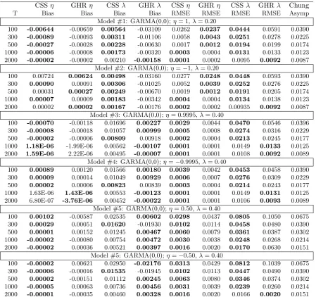
For the Monte Carlo experiments, we considered a total of eight different cases, including six GARMA(0,0) (Table 1) and two GARMA(1,0) models (Ta-ble 2). The true values of η are {−1,−0.9995,−0.50,0.50,0.9995,1} for the GARMA(0,0) cases. For |η| = 1, we fix λ = 0.20, where λ = 0.40 otherwise. For the GARMA(1,0) cases, we fixed λ= 0.40 and φ = 0.80, allowing the true values of η to be 0.50 and 0.9995. Note that the last model has short memory dynamics and is parametrically close to the non-stationary border. We thus an-ticipate that this model may produce relatively poor results. For each model, we performed 2500 simulations and considered sample sizes of 100, 300, 500, 1000, and 2000 observations. To generate a data series, xt, we calculated the autoco-variances of the long memory processes and obtained the Cholesky factorization of the Toeplitz matrix.4 This factorization is then multiplied by a sequence of nor-mal random variates of the desired length. Data are generated through recursion for each GARMA(1,0) case, whereµ is set to 0 throughout.
Tables 1-2 report the results of the mean bias and RMSE for each model and both the time domain estimator of Chung (CSS) and the frequency-based esti-mator ofGiraitis et al.(2001) (GHR). To help interpret the results, the estimator that yields the smallest bias/RMSE in absolute value for a given sample size is shown in bold type. For both estimators, the absolute value of the mean bias associated with η is remarkably small, with a value that decreases rapidly with the sample size. The CSS outperforms the GHR estimator in terms of the mean bias ofη. There are instances where the improvement in mean and RMSE can be somewhat large, especially when|η|= 0.50, likely resulting from the fact that the true value ofη is not typically in the discrete parameter space for the GHR estimator (except whenν is 0 or π). Whenν 6= 0, the GHR estimator tends to dominate in mean bias forλ. In terms of RMSE, for|η| 6= 1, the CSS estimator tends to dominate for η, λ, and in the cases of the GARMA(1,0) model, for φ
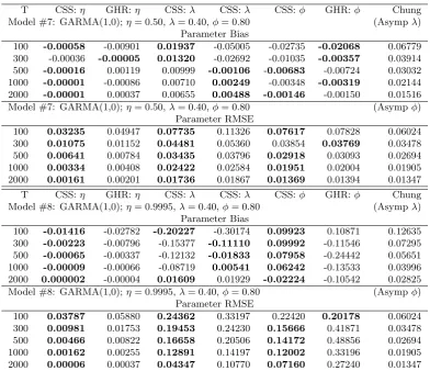
as well. It should be noted that the RMSE for both estimators of λ and φ are generally quite similar, and compare favorably with the computed asymptotic standard deviations of these parameters from Chung (1996b), Theorem 3, with one exception. In particular, performance of the estimators for the GARMA(1,0) model with η = 0.9995, λ = 0.40, and φ = 0.80 tends to be quite poor. For sample sizes less than 2000, the CSS and GHR procedures can result in a mean bias for λof -0.2023 and -0.3017, respectively. A similar picture emerges for φ, where the mean bias ofφcan be as large as 0.0992 for the CSS estimator, while the GHR estimator tends to underestimateφwith a mean bias that is typically quite large in absolute value. The results for the GARMA(1,0) cases show that
4
the mean bias inλtends to be inversely related to the mean bias inφ, especially for the CSS estimator. As is well known to researchers using parametric esti-mators in the ARFIMA context, it can be difficult to distinguish high frequency components from low frequency pieces (Nielsen and Frederiksen 2005).
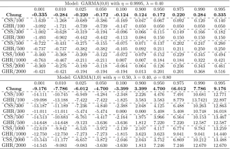
For researchers interested in obtaining point estimates for GARMA param-eters, andη specifically, the GHR and CSS estimators appear to provide highly robust options. However, the question remains as to whether or not proposed distribution theory can be used for inference and the construction of confidence bands. To this end, Table 3 displays the estimated and theoretical percentiles from two potentially problematic cases, one with η near 1 and another with an autoregressive component.5 Below the reported sample size, we present the per-centiles of the distribution of the statistic calculated fromChung(1996a), using his equation 19 and Table 1, along with the empirical distribution of the same quantity resulting from both the CSS and GHR estimators.
We are primarily interested in the CSS estimator, noting two things regarding the GHR estimator. First, the empirical distribution ofT(ˆη−η) for the GHR es-timator confirms the established convergence rate ofT as shown byGiraitis et al.
(2001). Second, we note that for the GHR estimator, the underlying parameter space is discrete. Consider for example, the empirical distribution of T(ˆη−η) when the true values ofη and λ are 0.9995 and 0.40 for a sample size equal to 300. Of the estimated 2500 values of η, 1162 are exactly equal to 0.99912, the closest possible value to 0.9995. While the estimator unquestionably performs well, this discretization can naturally result in small biases, which again helps to explain the findings in Tables 1-2, where the CSS estimator tends to dominate. It additionally highlights a potential concern in using a CSS-based algorithm that establishes a line search forηusing a discrete set as inChung(1996a) and Wood-ward et al.(1998). In what follows, we concentrate on the properties of the CSS estimator and algorithm proposed here.
For the two cases in Table 3, we generally see that the CSS estimator ofη has an empirical distribution that is well approximated by the asymptotic distribution provided byChung(1996a,b). The values of the empirical percentiles are typically quite close to the reported percentiles of Chung, especially for the 2.5% and 5.0% levels, which are important for statistical testing. Based on 500 observations, for example, withη = 0.50 and φ 6= 0, the empirical 5th percentile for T(ˆη−η) is -4.41, which closely matches the proposed theoretical quantity equal to -4.70.6
5
For brevity, we do not include all results from Tables 1 and 2, which are available upon request. Briefly summarizing, they provide conclusions that are qualitatively identical to those reported in Table 3 for the other parameterizations, except perhaps the case whereφ = 0.80 andη= 0.9995. Here, not surprisingly, for small samples, we find the distribution of is skewed left.
6
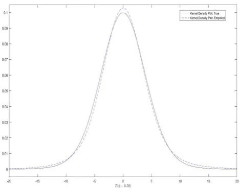
In spite of generally confirming the proposed distributional results, Table 3 hints that the finite sample distribution may have a more peaked density and fatter tails than theory implies. Consider Figure 1, which provides kernel density plots of 2000(ˆη−η) and the corresponding theoretical quantity using the dis-tribution theory for the CSS estimator based on the GARMA(0,0) model with
η = 0.50 and λ = 0.40.7 Indeed, the figure shows that there are several places
where the associated kernel density plots cross, suggesting that in finite samples, the empirical distribution may have larger kurtosis and a more peaked density than implied by theory. We now turn to the question of whether these issues impact the practical usefulness of the distributional results in constructing con-fidence bands.
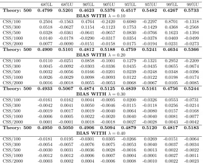
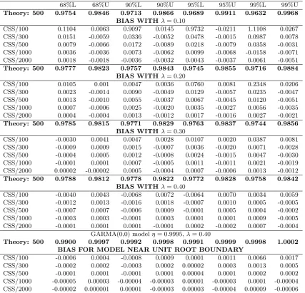
A large number of simulations generally reveal that theoretical confidence bands provide remarkably accurate coverage relative to empirical counterparts when |η| is in the neighborhood of unity and/or λ is near the non-stationary boundary. However, there can be very serious concerns with the use of theory, especially whenT is small and λis near 0. Tables 4 and 5 highlight these issues, where we present the associated biases that would result from the use of theory in constructing confidence bands. More specifically, the tables report the difference between the theoretical value ofηat the upper and lower 68%, 90%, 95%, and 99% confidence bands and the associated empirical quantity based on 5000 simulated values for GARMA(0,0) models withη= 0.50 and 0.98. For each value ofη, we allowλto take on the values{0.1,0.2,0.3,0.4}, and as above, we consider several sample sizes ranging from 100 to 2000. As a reference, the theoretical bands for sample sizes of 500 observations are presented in bold font.
From Table 4, we see that the amplified empirical kurtosis is especially prob-lematic for smallT and λ. Generally speaking, the 99% bands appear to be un-informative whenλ= 0.10, even for moderately large sample sizes. For T = 500, for example, 0.5% of estimated values of η are less than 0.2295, which starkly contrasts the theoretical value of 0.4799. Although somewhat reliable results can be obtained for 68% bands and sample sizes of at least 1000, the results with
λ= 0.10 show that the existing theory may need to be exercised with some cau-tion. We do note that the time series withλ= 0.10 might be viewed as somewhat extreme here, in light of the fact that they display characteristics that are difficult to distinguish from short memory. The theoretical first order autocorrelation co-efficient, for example, is 0.1015, and after the first lag, there is no value in excess of 0.05 in absolute value.
example the empirical 5thpercentile T(ˆη−η) is -4.11. The results support the proposed
inde-pendence ofηfrom other parameters.
7
We use a Gaussian smoothing window and a bandwidth parameter of 3. To calculate the theoretical density, one needs the associated percentiles ofY0 from (5). These values have been
Remaining results generally support the use of CSS theory for construction of confidence bands, especially for samples larger than 100 and narrower bands. Overall, biases rapidly decrease with both sample size and the value of λ. With
T = 2000 and λ = 0.40, as an example, 95% of all estimated values of η lie between 0.4962 and 0.5040, implying confidence bands for estimated cycles of between 5.975 and 6.0266 periods. These values are remarkably close to those implied by theory, where theoretical bands of 0.4970-0.5030 correspond to cycle lengths between 5.98 and 6.02 periods.
The results in Table 5 indicate that generally small biases in calculating confi-dence intervals with asymptotic quantities further decline asη approaches unity. Here for all cases, except when λ= 0.10 and T is smaller than 500, the empir-ical coverage areas are very well captured by asymptotic quantities. Especially when λ is large, the differences between empirical percentiles and the theoret-ical quantities becomes negligible. Displayed in the final panel in Table 5, we present results with λ = 0.40 where η = 0.9995, a parameterization very close to a unit root. Except in the case of the 99% confidence bands withT = 100, the associated biases are never greater than 0.0013 and are essentially zero for
T >1000.8
4. Hypothesis Testing for η
Overall, the results indicate that the proposed distribution theory for max-imum likelihood-based estimators works well in constructing confidence bands as |η| → 1. The question remains as to whether these results are useful for statistical testing purposes. Here, as recently emphasized by Dissanayake et al.
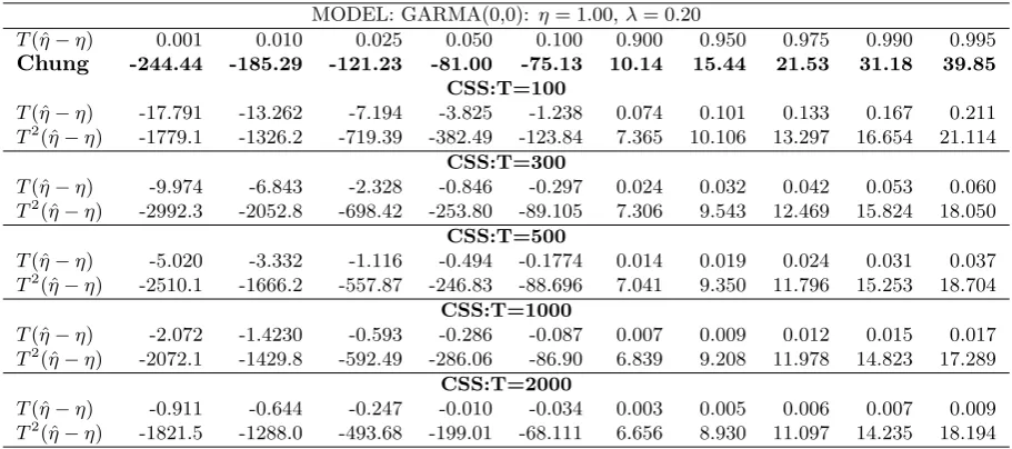
(2018), there are several specific hypotheses of interest, including H0 : η = 1 versusHA:η <1. Regrettably, as discussed above, a discontinuity exists in the proposed theory of Chung(1996a), such that we anticipate potential inferential problems. These concerns are validated in Table 6, which depicts the empirical distribution of the CSS estimator standardized by bothT andT2 when the true value ofη is 1.
Turning to the specific percentile values, we note that the empirical distribu-tion ofT2(ˆη−1) does not match the proposed asymptotic distribution of Chung (1996a). For example, in Table 6, the value of the empirical 1st percentile for
T2(ˆη−1) can be more than 11 times larger than the value established by Chung.
8
In other words, the empirical distribution is dramatically more skewed left than the theoretical results would imply. Further, the empirical distribution takes on fewer positive entries than the proposed asymptotic distribution. For example, the value associated with the 99th percentile from Chung’s asymptotic distribu-tion forT2(ˆη−1) is 31.13. Based on a sample size of 300, this implies that when
η= 1, 1% of all estimates of this parameter will be at least 1.00035. In contrast, the empirical distribution shows that only 1% of all values exceed 1.00018.
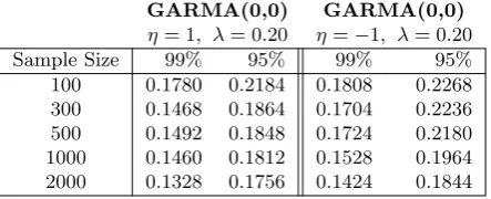
To analyze how empirical and theoretical distributional disparities impact inference, we consider the proposed tests ofChung(1996a,b) in Table 7 for|η|= 1, when the true value ofη is 1 or -1. The hypothesis can be tested by constructing confidence intervals about the estimate of η, where an ARFIMA process cannot be rejected if the value of unity lies within the confidence interval. The left-hand side of Table 7 reports the empirical size based on the 95% and 99% confidence intervals when the true value ofηis 1, while the right hand side of Table 7 presents the same results whenη=−1. Note, the confidence intervals are constructed here using the distributional results withT2rate of convergence when|η|= 1 (see (6)). The table shows that the implementation of the proposed distribution theory under the null will result in massive size distortion, with only mild relief as the sample size increases. Consider the case where the generated data are ARFIMA processes withη= 1. Even with 2000 observations and a 5% test, the constructed theoretical confidence bands underH0fail to include unity 17.6% of the time. The rejection rates of the true nullη = 1 can be larger than 20%. Moving to the 99% confidence intervals (e.g. a 1% test), we still see that the rejection rates exceed 13%. Throughout, the results are slightly worse when η = −1. For even large samples, these results suggest that the proposed distributional theory is unlikely to be useful to researchers interested in determining if the true data generating process is an ARFIMA or GARMA process. This can be especially problematic for those interested in testing for stationarity, where non-stationarity occurs for all values ofλ ≥ 0.25 when |η| = 1, but only occurs when λ ≥ 0.50 otherwise. Clearly, suitable testing procedures are needed. We offer two possibilities that we wish to posit as potential avenues for future work.
test size that assumes rateT convergence, yielded rejection rates of 6.64%, 5.28%, 4.84%, 5.44%, and 4.36%, respectively.
A more formal test that is potentially preferred has recently been advocated by Dissanayake et al. (2018), who discuss the use of quasi-likelihood ratio test statistics based on a state space representation of the GARMA model. Following a similar approach, one could obtain the value of the likelihood function in (4), with and withoutη= 1 imposed, and form the test statistic as follows,
LR= 2
max φ′,θ′,λ,η,µL(φ
′
, θ′
, λ, η, µ)− max φ′,θ′,λ,µL(φ
′
, θ′
, λ,1, µ)
. (11)
Under the null, the value of η lies on the boundary of the parameter space, and given the difficulties above, it seems likely that the distribution of the resulting test statistic will be non-standard. In light of the problems with the existing theory, as discussed here, computational methods may be preferred.
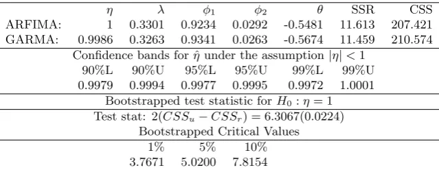
As a reasonable approach, one could use the estimated model under the null hypothesis to form a parametric bootstrap. Data of the desired length could be simulated based on sampling with replacement from the residuals of the null model, and the critical values of the distribution could be formed based on the test statistic in (11). This procedure was applied to the unemployment rate data described in Section2, using the residuals from an estimated ARFIMA(2,1) model. Results, which are based on 5000 simulations, are presented in Table 7.9 Here, we see that the likelihood ratio test statistic associated with the hypothesis
η= 1 takes on a value of 6.31, exceeding simulated critical values at the 5%, but not at the 1% levels. As discussed above, these findings are likely of tremendous importance to applied researchers in economics, since the null model is non-stationary, but strong stationary cycles result under the alternative.
The results provide reasonably strong support favoring|η|<1 and also high-light the difficulties that could be encountered for researchers employing CSS theory. More specifically, confidence bands constructed under the null hypothe-sis |η|= 1 suffer from such severe size distortion they are likely uninformative. For the example here, a more careful testing analysis shows a marginal rejection of η = 1 , whereas strong rejection occurs for virtually any size when using the theory ofChung(1996a,b) based on the assumedT2 rate of convergence. Finally, we see that the associated theoretical confidence bands under|η|<1 only contain unity when considering 99% intervals, matching the likelihood ratio test results. In instances where a parametric bootstrap is not available, these findings suggest that more conservative bands may be informative in determining if long memory
9
For computational purposes, and given the non-stationarity of the null model, the data are simulated recursively using the coefficients of the expansion of (1−L)−0.3301
cycles have finite length.
5. Conclusions
Considerable attention has recently focused on the use of models that allow for long memory cycles and potential singularities in the spectral density function, notably Gegenbauer autoregressive moving (GARMA) and associated k-factor GARMA models. While a number of robust estimators appears to exist in the time and frequency domain, it does not appear that there are an accepted set of distributional results related to the parameter, or parameters in the case of k-factor models, dictating the cycle length and the positions of spectral poles.
In this manuscript, we analyze the performance of two relevant likelihood-based estimators, where at least partial distributional results have been proposed. This includes, the Whittle estimator (GHR) described by Giraitis et al.(2001), and the approximate maximum likelihood estimator (CSS) analyzed by Chung
(1996a,b). While Giraitis et al. (2001) were able to prove rate-T convergence of the estimator of the pole, they were unable to provide an exact limiting distri-bution given its discrete nature. To date, only Chung (1996a,b) has proposed an approximate maximum likelihood estimator that could be used for statistical inference and the calculation on confidence bands. However, the results were obtained without a formal consistency proof, given complications in the distri-bution theory, including the fact that the relevant parameter space is closed and the proposed distribution appears to have a potential discontinuity. The pro-posed theory is potentially relevant for other likelihood-based estimators, serving at least as a reference point, and has recently been extended byBeaumont and Smallwood(2019) andPeiris and Asai(2016) to accommodate multiple poles and heteroskedastic disturbances. It is therefore imperative to understand the extent to which the proposed asymptotic theory is relevant.
Using a double gradient-based search algorithm, an extensive Monte Carlo analysis revealed that both estimators are highly robust in estimating model pa-rameters, specifically the position of the spectral pole and its associated cosine, denoted η. As the CSS estimator admits a continuous parameter space, it is found to be relatively superior in estimation ofη. Empirical results very strongly support the proposed distribution theory of Chung(1996a,b) for stationary pa-rameterizations in a neighborhood of a unit root process, especially for larger samples. Additionally, in most cases, the distribution theory is shown to be quite useful in constructing confidence bands, where empirical coverage areas are sometimes surprisingly well captured by associated asymptotic quantities.
sim-ulation results show that constructed wider confidence bands are likely to be uninformative under very weak long memory in samples less than 500 observa-tions. From a practical perspective, we would recommend the avoidance of the proposed asymptotic theory for very small samples when weak persistence is sus-pected, perhaps as evidenced by a differencing parameter in the neighborhood of zero. Otherwise, narrower confidence bands are generally found to be robust, such that we would also recommend using multiple sets of intervals when presenting theoretical results.
From a testing perspective, we further show that the proposed distribution theory under the null|η|= 1 would render severe size distortion and can cause confusion regarding whether a series is a stationary GARMA process or non-stationary ARFIMA/unit root process. This does not appear to be a small prob-lem, with rejection rates under the null approaching 20% for a 5% test size in samples of about 2000. We are able to demonstrate however, that the more conservative use of theory under the assumption|η|<1 may be useful in distin-guishing ARFIMA/ARIMA processes from GARMA counterparts.
The paper concludes with an application to unemployment, where evidence using a parametric bootstrap provides support for the existence of stationary, long memory cycles in the labor market. The overall conclusions suggest that GARMA parameters can be well estimated by existing likelihood-based tech-niques. For researchers interested in obtaining confidence bands for cycle lengths and conducting inference, the existing theory also appears to be largely applica-ble. Nonetheless, the results also show there are still several gaps in the existing theory that merit additional exploration, specifically as it relates to testing for
|η|in the neighborhood of 1. Awaiting additional distributional results, we sus-pect computational methods are most likely to be informative for researchers interested in statistical inference.
References
Arteche, J. and Robinson, P. M. (2000). Semiparametric inference in seasonal and cyclical long memory processes. Journal of Time Series Analysis, 21(1):1–25.
Artiach, M. and Arteche, J. (2012). Doubly fractional models for dynamic heteroscedastic cycles. Computational Statistics & Data Analysis, 56(6):2139 – 2158.
Asai, M., Peiris, S., McAleer, M., and Allen, D. (2018). Cointegrated dynamics for a gener-alized long memory process: An application to interest rates. Technical Report EI2018-32, Econometric Institute Research Papers, University of Madrid.
Beaumont, P. M. and Smallwood, A. D. (2019). Constrained sum of squares estimation of multiple frequency long memory models. Working Paper, Florida State University.
Caporale, G. M. and Gil-Alana, L. (2014). Long-run and cyclical dynamics in the US stock market. Journal of Forecasting, 33(2):147–161.
Chung, C.-F. (1996a). Estimating a generalized long memory process.Journal of Econometrics, 73(1):237 – 259.
Chung, C.-F. (1996b). A generalized fractionally integrated autoregressive moving average pro-cess. Journal of Time Series Analysis, 17:111–140.
Diongue, A. K. and Ndongo, M. (2016). The k-factor GARMA process with infinite variance innovations. Communications in Statistics-Simulation and Computation, 45(2):420–437. Dissanayake, G. S., Peiris, M. S., and Proietti, T. (2018). Fractionally differenced Gegenbauer
processes with long memory: A review. Statistical Science, 33(3):413–426.
Ferrara, L. and Gu´egan, D. (2001). Forecasting with k-factor Gegenbauer processes: Theory and applications. Journal of Forecasting, 20(8):581–601.
Geweke, J. and Porter-Hudak, S. (1983). The estimation and application of long memory time series models. Journal of Time Series Analysis, 4(4):221–238.
Gil-Alana, L. A. (2007). Testing the existence of multiple cycles in financial and economic time series. Annals of Economics & Statistics, 8(1):1–20.
Giraitis, L., Hidalgo, J., and Robinson, P. M. (2001). Gaussian estimation of parametric spectral density with unknown pole. The Annals of Statistics, 29(4):987–1023.
Granger, C. W. J. and Joyeux, R. (1980). An introduction to long-memory time series models and fractional differencing. Journal of Time Series Analysis, 1(1):15–24.
Gray, H. L., Zhang, N., and Woodward, W. A. (1989). On generalized fractional processes. Journal of Time Series Analysis, 10:233–257.
Hidalgo, J. (2005). Semiparametric estimation for stationary processes whose spectra have an unknown pole. The Annals of Statistics, 33(4):1843–1889.
Hidalgo, J. and Soulier, P. (2004). Estimation of the location and exponent of the spectral singularity of a long memory process. Journal of Time Series Analysis, 25(1):55–81. Hosking, J. R. M. (1981). Fractional differencing. Biometrika, 68:165–76.
Leschinski, C. and Sibbertsen, P. (2019). Model order selection in periodic long memory models. Econometrics and Statistics, 9:78 – 94.
Lu, Z. and Guegan, D. (2011). Estimation of time-varying long memory parameter using wavelet method. Communications in Statistics—Simulation and Computation, 40(4):596–613. McElroy, T. S. and Holan, S. H. (2012). On the computation of autocovariances for generalized
Gegenbauer processes. Statistica Sinica, 22(4):1661–1687.
Nielsen, M. Ø. and Frederiksen, P. H. (2005). Finite sample comparison of parametric, semipara-metric, and wavelet estimators of fractional integration.Econometric Reviews, 24(4):405–443. Peiris, M. and Asai, M. (2016). Generalized fractional processes with long memory and time
dependent volatility revisited. Econometrics, 4(4):37.
Ramachandran, R. and Beaumont, P. (2001). Robust estimation of GARMA model param-eters with an application to cointegration among interest rates of industrialized countries. Computational Economics, 17(2/3):179–201.
Reisen, V. A., Zamprogno, B., Palma, W., and Arteche, J. (2014). A semiparametric approach to estimate two seasonal fractional parameters in the SARFIMA model. Mathematics and Computers in Simulation, 98:1 – 17.
Robinson, P. M. (1995). Log-periodogram regression of time series with long range dependence. The Annals of Statistics, 23(3):1048–1072.
Woodward, W. A., Cheng, Q. C., and Gray, H. L. (1998). A k-factor GARMA long-memory model. Journal of Time Series Analysis, 19(485-504).
Table 1: Bias and RMSE for Whittle and CSS estimates of GARMA(0,0) model parameters
CSSη GHRη CSS λ GHRλ CSSη GHRη CSSλ GHRλ Chung
T Bias Bias Bias Bias RMSE RMSE RMSE RMSE Asymp Model #1: GARMA(0,0);η= 1,λ= 0.20
100 -0.00644 -0.00659 0.00564 -0.03109 0.0262 0.0237 0.0444 0.0591 0.0390 300 -0.00089 -0.00093 0.00311 -0.01106 0.0058 0.0043 0.0251 0.0278 0.0225 500 -0.00027 -0.00028 0.00228 -0.00630 0.0017 0.0012 0.0194 0.0199 0.0174 1000 -0.00006 -0.00008 0.00173 -0.00320 0.0003 0.0004 0.0131 0.0133 0.0123 2000 -0.00002 -0.00002 0.00210 -0.00158 0.0001 0.0002 0.0095 0.0092 0.0087
Model #2: GARMA(0,0);η=−1,λ= 0.20
100 0.00724 0.00624 0.00498 -0.03160 0.0277 0.0248 0.0448 0.0593 0.0390 300 0.00090 0.00091 0.00306 -0.01025 0.0052 0.0039 0.0252 0.0276 0.0225 500 0.00031 0.00027 0.00249 -0.00670 0.0019 0.0012 0.0191 0.0205 0.0174 1000 0.00007 0.00009 0.00183 -0.00342 0.0004 0.0004 0.0134 0.0138 0.0123 2000 0.00002 0.00002 0.00167 -0.00176 0.0002 0.0002 0.00935 0.0092 0.0087
Model #3: GARMA(0,0);η= 0.9995,λ= 0.40
100 -0.00070 -0.00118 0.01696 0.00227 0.0029 0.0044 0.0470 0.0546 0.0396 300 -0.00008 -0.00018 0.01057 0.00999 0.0005 0.0008 0.0274 0.0316 0.0229 500 -0.00002 -0.00006 0.00809 0.00918 0.0002 0.0004 0.0213 0.0245 0.0177 1000 1.18E-06 -1.99E-06 0.00562 -0.00107 0.0001 0.0001 0.0149 0.0133 0.0125 2000 1.59E-06 2.22E-06 0.00495 -0.00007 0.0001 0.0001 0.0108 0.0092 0.0089
Model #4: GARMA(0,0);η=−0.9995,λ= 0.40
100 0.00089 0.00120 0.01566 0.00180 0.0039 0.0042 0.0453 0.0458 0.0390 300 0.00009 0.00014 0.01049 0.00929 0.0006 0.0007 0.0276 0.0309 0.0229 500 0.00002 0.00006 0.00823 0.00839 0.0003 0.0004 0.0214 0.0243 0.0177 1000 1.63E-06 1.43E-06 0.00553 -0.00123 0.0001 0.0001 0.0149 0.0131 0.0125 2000 6.80E-07 -3.76E-06 0.00452 -0.00022 0.0001 0.0001 0.0106 0.0093 0.0089
Model #5: GARMA(0,0);η= 0.50,λ= 0.40
100 0.00102 -0.00587 0.02535 0.00602 0.0298 0.0437 0.0805 0.1050 0.0675 300 0.00029 0.00051 0.01620 -0.01930 0.0102 0.0114 0.0458 0.0480 0.0390 500 0.00001 0.00152 0.01245 0.00467 0.0060 0.0079 0.0361 0.0387 0.0302 1000 -0.00002 -0.00080 0.00754 0.00472 0.0030 0.0038 0.0248 0.0268 0.0214 2000 -0.00002 0.00036 0.00521 0.00397 0.0016 0.0020 0.0170 0.0630 0.0151
Model #5: GARMA(0,0);η=−0.50,λ= 0.40
Table 2: Bias and RMSE for Whittle/CSS based estimates of the GARMA(1,0) model
T CSS:η GHR:η CSS:λ CSS:λ CSS:φ GHR:φ Chung Model #7: GARMA(1,0);η= 0.50,λ= 0.40,φ= 0.80 (Asympλ)
Parameter Bias
100 -0.00058 -0.00901 0.01937 -0.05005 -0.02735 -0.02068 0.06779 300 -0.00036 -0.00005 0.01320 -0.02692 -0.01035 -0.00357 0.03914 500 -0.00016 0.00119 0.00999 -0.00106 -0.00683 -0.00724 0.03032 1000 -0.00001 -0.00086 0.00710 0.00249 -0.00348 -0.00319 0.02144 2000 -0.00001 0.00037 0.00655 0.00488 -0.00146 -0.00150 0.01516 Model #7: GARMA(1,0);η= 0.50,λ= 0.40,φ= 0.80 (Asympφ)
Parameter RMSE
100 0.03235 0.04947 0.07735 0.11326 0.07617 0.07828 0.06024 300 0.01075 0.01152 0.04481 0.05360 0.03854 0.03769 0.03478 500 0.00641 0.00784 0.03435 0.03796 0.02918 0.03093 0.02694 1000 0.00334 0.00408 0.02422 0.02584 0.01951 0.02004 0.01905 2000 0.00161 0.00201 0.01736 0.01867 0.01369 0.01394 0.01347 T CSS:η GHR:η CSS:λ CSS:λ CSS:φ GHR:φ Chung Model #8: GARMA(1,0);η= 0.9995,λ= 0.40,φ= 0.80 (Asympλ)
Parameter Bias
100 -0.01416 -0.02782 -0.20227 -0.30174 0.09923 0.10871 0.12635 300 -0.00223 -0.00796 -0.15377 -0.11110 0.09992 -0.11546 0.07295 500 -0.00065 -0.00337 -0.12132 -0.01833 0.07958 -0.24442 0.05651 1000 -0.00009 -0.00066 -0.08719 0.00541 0.06242 -0.13533 0.03996 2000 0.000002 -0.00004 0.01609 0.01929 -0.02224 -0.10542 0.02825 Model #8: GARMA(1,0);η= 0.9995,λ= 0.40,φ= 0.80 (Asympφ)
Parameter RMSE
100 0.03787 0.05880 0.24362 0.33197 0.22420 0.20178 0.06024 300 0.00981 0.01753 0.19453 0.24230 0.15666 0.41871 0.03478 500 0.00466 0.00822 0.16658 0.20506 0.14172 0.48856 0.02694 1000 0.00162 0.00255 0.12891 0.14197 0.12002 0.33196 0.01905 2000 0.00006 0.00037 0.04347 0.10770 0.07160 0.27240 0.01347
Table 3: Empirical distribution for the percentilesT(ˆη−η)
.
Model: GARMA(0,0) withη= 0.9995,λ= 0.40
0.001 0.010 0.025 0.050 0.100 0.900 0.950 0.975 0.990 0.995
Chung -0.335 -0.284 -0.220 -0.172 -0.124 0.124 0.172 0.220 0.284 0.335
CSS/100 -1.639 -1.268 -0.689 -0.386 -0.169 0.047 0.067 0.092 0.120 0.140
GHR/100 -3.092 -1.721 -0.739 -0.739 -0.147 0.050 0.050 0.050 0.050 0.050
CSS/300 -1.002 -0.628 -0.319 -0.194 -0.096 0.066 0.115 0.149 0.166 0.182
GHR/300 -1.493 -0.902 -0.442 -0.442 -0.113 0.084 0.150 0.150 0.150 0.150
CSS/500 -0.722 -0.431 -0.275 -0.155 -0.075 0.071 0.137 0.202 0.247 0.260
GHR/500 -0.737 -0.737 -0.382 -0.382 -0.105 0.092 0.211 0.211 0.250 0.250
CSS/1000 -0.460 -0.368 -0.209 -0.122 -0.072 0.079 0.152 0.229 0.345 0.494
GHR/1000 -0.763 -0.467 -0.211 -0.211 0.007 0.007 0.184 0.184 0.322 0.421
CSS/2000 -0.369 -0.276 -0.189 -0.118 -0.064 0.064 0.126 0.236 0.343 0.461
GHR/2000 -0.421 -0.421 -0.194 -0.194 -0.194 0.013 0.201 0.201 0.368 0.516
Model: GARMA(1,0) withη= 0.50,λ= 0.40,φ= 0.80
0.001 0.010 0.025 0.050 0.100 0.900 0.950 0.975 0.990 0.995
Chung -9.176 -7.786 -6.012 -4.700 -3.399 3.399 4.700 66.012 7.786 9.176
CSS/100 -14.111 -10.745 -6.949 -4.284 -2.348 2.226 4.476 7.491 10.681 12.771
GHR/100 -19.098 -13.188 -7.422 -7.422 -1.825 3.583 3.583 8.779 13.7421 22.897
CSS/300 -13.187 -11.189 -7.236 -4.840 -2.388 2.048 4.125 6.488 10.263 12.863
GHR/300 -11.011 -11.011 -5.474 -5.474 0.000 0.000 5.408 5.408 10.748 16.018
CSS/500 -14.513 -10.683 -6.761 -4.417 -2.164 1.975 3.966 6.564 10.153 13.467
GHR/500 -14.648 -14.648 -9.123 -3.636 -3.636 1.812 7.220 7.220 12.587 12.587
CSS/1000 -12.619 -9.842 -6.535 -3.972 -2.139 2.107 4.117 6.774 9.783 13.259
GHR/1000 -12.750 -12.750 -7.273 -7.273 -1.815 3.623 3.623 9.041 9.041 14.440
CSS/2000 -15.543 -11.177 -6.657 -3.872 -2.046 2.043 3.752 6.869 10.212 13.488
GHR/2000 -14.545 -9.083 -9.083 -3.630 -3.630 1.813 7.246 7.246 12.670 12.670
Notes: In bold font, we present the values at theoretical percentiles for the test statistic using equation (4) and the associated simulated quantities forY0 fromChung(1996a). The remaining elements yield the
Table 4: Bias in estimating confidence bands in GARMA(0,0) models withη= 0.05.
68%L 68%U 90%L 90%U 95%L 95%U 99%L 99%U
Theory: 500 0.4799 0.5201 0.4623 0.5376 0.4517 0.5482 0.4267 0.5733 BIAS WITH λ= 0.10
CSS/100 0.2504 -0.1563 0.4764 -0.2420 0.6080 -0.2297 0.8701 -0.1318 CSS/300 0.0518 -0.0627 0.1154 -0.1123 0.1753 -0.1429 0.4368 -0.2568 CSS/500 0.0328 -0.0361 -0.0641 -0.0657 0.0830 -0.0766 0.1623 -0.1394 CSS/1000 0.0140 -0.0178 -0.0290 -0.0317 0.0354 -0.0378 0.0469 -0.0499 CSS/2000 0.0077 -0.0090 -0.0151 -0.0158 0.0175 -0.0194 0.0231 -0.0273
Theory: 500 0.4900 0.5101 0.4812 0.5188 0.4759 0.5241 0.4634 0.5366 BIAS WITH λ= 0.20
CSS/100 0.0110 -0.0251 0.0858 -0.1001 0.1279 -0.1321 0.2952 -0.2209 CSS/300 0.0045 -0.0092 -0.0303 -0.0336 0.0435 -0.0435 0.0655 -0.0674 CSS/500 0.0032 -0.0056 0.0166 -0.0201 0.0239 -0.0248 0.0348 -0.0396 CSS/1000 0.0026 -0.0029 0.0098 -0.0093 0.0122 -0.0122 0.0198 -0.0174 CSS/2000 0.0016 -0.0018 0.0055 -0.0053 0.0068 -0.0067 0.0105 -0.0085
Theory: 500 0.4933 0.5067 0.4874 0.5125 0.4839 0.5161 0.4756 0.5244 BIAS WITH λ= 0.30
CSS/100 -0.0161 0.0162 0.0044 -0.0095 0.0200 -0.0326 0.0553 -0.0731 CSS/300 -0.0042 0.0041 0.0050 -0.0046 -0.0115 -0.0118 0.0256 -0.0214 CSS/500 -0.0019 0.0017 0.0019 -0.0040 0.0064 -0.0080 0.0157 -0.0168 CSS/1000 -0.0006 0.0005 0.0022 -0.0020 0.0040 -0.0040 0.0081 -0.0077 CSS/2000 0.0001 -0.0001 0.0018 -0.0018 0.0027 -0.0028 0.0043 -0.0042
Theory: 500 0.4950 0.5050 0.4906 0.5094 0.4879 0.5120 0.4817 0.5183 BIAS WITH λ= 0.40
CSS/100 -0.0181 0.0195 -0.0301 0.0305 -0.0266 0.0269 -0.0151 -0.0064 CSS/300 -0.0054 -0.0057 -0.0076 0.0075 -0.0053 0.0040 0.0037 -0.0034 CSS/500 -0.0030 0.0031 -0.0036 0.0028 -0.0016 0.0013 0.0022 -0.0022 CSS/1000 -0.0012 0.0012 -0.0006 0.0007 0.0004 -0.0001 0.0027 -0.0011 CSS/2000 -0.0003 0.0002 0.0004 -0.0006 0.0008 -0.0010 0.0022 -0.0023 Notes: The table reports the difference between the value ofηassociated with theoretical confidence bands, which have been constructed using equation (5) along with simulated values forY0, and the estimated value
Table 5: Bias in estimating confidence bands in GARMA(0,0) models withη= 0.98.
68%L 68%U 90%L 90%U 95%L 95%U 99%L 99%U
Theory: 500 0.9754 0.9846 0.9713 0.9866 0.9689 0.9911 0.9632 0.9968 BIAS WITH λ= 0.10
CSS/100 0.1104 0.0063 0.9097 0.0145 0.9732 -0.0211 1.1108 0.0267 CSS/300 0.0151 -0.0059 0.0336 -0.0052 0.0478 -0.0015 0.0987 0.0078 CSS/500 0.0079 -0.0066 0.0172 -0.0089 0.0218 -0.0079 0.0358 -0.0031 CSS/1000 0.0036 -0.0036 0.0073 -0.0062 0.0099 -0.0068 -0.0158 -0.0071 CSS/2000 0.0018 -0.0018 -0.0036 -0.0032 0.0043 -0.0037 0.0061 -0.0051
Theory: 500 0.9777 0.9823 0.9757 0.9843 0.9745 0.9855 0.9716 0.9884 BIAS WITH λ= 0.20
CSS/100 0.0105 0.001 0.0047 0.0036 0.0760 0.0081 0.2348 0.0206 CSS/300 0.0023 -0.0014 0.0090 -0.0049 0.0129 -0.0057 0.0235 -0.0047 CSS/500 0.0013 -0.0010 0.0055 -0.0037 0.0067 -0.0045 0.0120 -0.0051 CSS/1000 0.0007 -0.0006 0.0025 -0.0020 0.0035 -0.0027 0.0056 -0.0035 CSS/2000 0.0004 -0.0004 0.0013 -0.0012 0.0017 -0.0016 0.0027 -0.0021
Theory: 500 0.9785 0.9815 0.9771 0.9829 0.9763 0.9837 0.9744 0.9856 BIAS WITH λ= 0.30
CSS/100 -0.0030 0.0041 0.0047 0.0028 0.0107 0.0020 0.0387 0.0081 CSS/300 -0.0009 0.0009 0.0015 -0.0007 0.0036 -0.0020 0.0071 -0.0028 CSS/500 -0.0004 0.0005 0.0012 -0.0008 0.0024 -0.0015 0.0047 -0.0030 CSS/1000 -0.0001 0.0001 0.0007 -0.0005 0.0011 -0.0011 0.0021 -0.0019 CSS/2000 0.00002 -0.00002 0.0005 -0.0004 0.0007 -0.0006 0.0013 -0.0012
Theory: 500 0.9788 0.9812 0.9778 0.9822 0.9772 0.9828 0.9758 0.9842 BIAS WITH λ= 0.40
CSS/100 -0.0040 0.0043 -0.0068 0.0072 -0.0064 0.0070 0.0034 0.0059 CSS/300 -0.0012 0.0013 -0.0016 0.0018 -0.0007 0.0010 0.0005 -0.0005 CSS/500 -0.0007 0.0007 -0.0006 0.0009 -0.0001 0.0005 0.0004 -0.0002 CSS/1000 -0.0003 0.0003 -0.0001 0.0003 0.0001 0.0001 0.0009 -0.0005 CSS/2000 -0.0001 0.0001 0.0001 -0.0001 0.0002 -0.0002 0.0007 -0.0004
GARMA(0,0) modelη= 0.9995,λ= 0.40
Theory: 500 0.9900 0.9997 0.9992 0.9998 0.9991 0.9999 0.9998 1.0002 BIAS FOR MODEL NEAR UNIT ROOT BOUNDARY
CSS/100 -0.0006 0.0004 -0.0008 0.0009 0.0001 0.0011 0.0066 0.0017 CSS/300 -0.0002 0.0002 -0.0003 0.0002 0.00002 0.0003 0.0013 0.0005 CSS/500 -0.0001 0.0001 -0.0001 0.0001 0.00004 0.0001 0.0002 0.0002 CSS/1000 -0.00005 0.00003 -0.00004 -0.00003 0.00001 -0.00003 0.0001 -0.00004 CSS/2000 -0.00002 0.000001 0.00001 -0.00003 0.00003 -0.00004 0.00009 -0.00006 Notes: The table reports the difference between the value ofηassociated with theoretical confidence bands, which have been constructed using equation (5) along with simulated values forY0, and the estimated value
Table 6: Percentiles forT(ˆη−η) andT2
(ˆη−η) for the empirical distribution ofηwhen|η|= 1.
MODEL: GARMA(0,0): η= 1.00,λ= 0.20
T(ˆη−η) 0.001 0.010 0.025 0.050 0.100 0.900 0.950 0.975 0.990 0.995 Chung -244.44 -185.29 -121.23 -81.00 -75.13 10.14 15.44 21.53 31.18 39.85
CSS:T=100
T(ˆη−η) -17.791 -13.262 -7.194 -3.825 -1.238 0.074 0.101 0.133 0.167 0.211 T2
(ˆη−η) -1779.1 -1326.2 -719.39 -382.49 -123.84 7.365 10.106 13.297 16.654 21.114
CSS:T=300
T(ˆη−η) -9.974 -6.843 -2.328 -0.846 -0.297 0.024 0.032 0.042 0.053 0.060 T2
(ˆη−η) -2992.3 -2052.8 -698.42 -253.80 -89.105 7.306 9.543 12.469 15.824 18.050
CSS:T=500
T(ˆη−η) -5.020 -3.332 -1.116 -0.494 -0.1774 0.014 0.019 0.024 0.031 0.037 T2
(ˆη−η) -2510.1 -1666.2 -557.87 -246.83 -88.696 7.041 9.350 11.796 15.253 18.704
CSS:T=1000
T(ˆη−η) -2.072 -1.4230 -0.593 -0.286 -0.087 0.007 0.009 0.012 0.015 0.017 T2
(ˆη−η) -2072.1 -1429.8 -592.49 -286.06 -86.90 6.839 9.208 11.978 14.823 17.289
CSS:T=2000
T(ˆη−η) -0.911 -0.644 -0.247 -0.010 -0.034 0.003 0.005 0.006 0.007 0.009 T2
(ˆη−η) -1821.5 -1288.0 -493.68 -199.01 -68.111 6.656 8.930 11.097 14.235 18.194 Notes: In bold font, we present the values at theoretical percentiles for the test statisticT2
(ˆη−η) using equation (6) and the associated simulated quantities forY1 fromChung(1996a). The remaining elements
Table 7: Rejection rates of the null hypothesis|η|= 1 using Chung’s confidence intervals
GARMA(0,0) GARMA(0,0)
η= 1, λ= 0.20 η=−1, λ= 0.20 Sample Size 99% 95% 99% 95% 100 0.1780 0.2184 0.1808 0.2268 300 0.1468 0.1864 0.1704 0.2236 500 0.1492 0.1848 0.1724 0.2180 1000 0.1460 0.1812 0.1528 0.1964 2000 0.1328 0.1756 0.1424 0.1844
Table 8: Results of parametric bootstrap applied to US unemployment
η λ φ1 φ2 θ SSR CSS
ARFIMA: 1 0.3301 0.9234 0.0292 -0.5481 11.613 207.421 GARMA: 0.9986 0.3263 0.9341 0.0263 -0.5674 11.459 210.574
Confidence bands for ˆηunder the assumption|η|<1 90%L 90%U 95%L 95%U 99%L 99%U 0.9979 0.9994 0.9977 0.9995 0.9972 1.0001
Bootstrapped test statistic forH0:η= 1
Test stat: 2(CSSu−CSSr) = 6.3067(0.0224)
Bootstrapped Critical Values 1% 5% 10% 3.7671 5.0200 7.8154
Notes: The ARFIMA model has been obtained with the restrictionη= 1 imposed. Given the functional relationshipd= 2λ, the model can be written as:
(1−L)0.6602
(1−0.923L−0.029L2
)(ut−6.20) = (1−0.548L)εt.