One Common Solution to the Singularity
and Perihelion Problems
Branko Sarić1,2
1Department of Mathematics and Informatics, Faculty of Sciences, University of Novi Sad, Novi Sad, Serbia 2College of Technical Engineering Professional Studies, Čačak, Serbia
Email: [email protected]
Received September 18, 2012; revised October 18, 2012; accepted October 25, 2012
ABSTRACT
With a view to surmounting the singularity problem on the one hand, as well as the moving perihelion problem of the planets on the other, as two acutely vexed questions within Newton’s gravity concept, the goal of this paper is a modifi-
cation of Newton’s gravity concept itself.
Keywords: Celestial Mechanics; Planets; Rings
1. Introduction
It would be difficult to exaggerate the influence of New- ton’s theory of gravitation on the subsequent develop-
ment of physics. As well as explaining Kepler’s laws of
planetary motion, Newton’s theory was central to the suc-
cessful mathematization of physics using the newly-in- vented calculus and it served as a paradigm for the later theories of electrostatics and magnetostatics. However, new insights into Milky Way satellite galaxies raise awk- ward questions for cosmologists: Do we have to modify
Newton’s theory of gravitation as it fails to explain so
many observations? In other words, although Newton’s
theory does, in fact, describe the everyday effects of gra- vity on Earth, things we can see and measure, it is con- ceivable that we have completely failed to comprehend the actual physics underlying the Newton’s force of grav-
ity. In addition, Newton’s theory does not fully explain
the precession of the perihelion of the orbits of the Plan-ets, especially of planet Mercury. Namely, it has been experimentally stated that the perihelion of Mercury’s or- bits moves into the plane of its planetary motion around the Sun. In other words, all planetary motions of Sun’s planetary system depart from elliptical orbits obtained from Newton’s gravity theory, [1]. By the strict Schwarz- shild-Droste’s solution to the static gravitational field
with spherical symmetry, in the general Einstein’s rela-
tivity theory, the perihelion problem has been approxi- mately solved, [1]. On the other hand, Einstein’s theory
has some difficulties hard to be overcome such as the problem of singularity, that occurs in Newton’s theory too
(all relevant physical variables, such as velocity, force, kinetic and potential energy, don’t exist at point of sin-
gularity). Accordingly, in order to solve simultaneously these two acutely vexed questions within Newton’s grav-
ity theory, we present, in this research paper, an ap- proximative modification of Newton’s gravity concept
itself. The outline of this article is as follows: In the Pre- liminaries, the space-time continuum (the integral space), as an ambient space, is completely defined. In Section 1 we establish a causal connection between the expression for the kinetic energy of a material point and the Min- kowski metric in the four-dimensional space-time con- tinuum. In addition, in two separate subsections of this section we derive Newton’s equations of motion and the
relativistic Hamilton-Jacobi equation for a free particle. Since the dynamic (Newton’s) equations of motion are
formally derived from geodesic equations in Section 2, this section together with Appendix at the end of the pa- per provide a possibility of further work on the modifica- tion of Newton’s gravity theory in Section 3. In this last
section we show that a comprehensive analysis of parti- cle motion under the modified Newton’s gravity force
leads to the perihelion motions of a Planet’s elliptical
orbit.
2. Preliminaries
By a material point , introduced for the purpose of an useful idealization, one means a geometrical point, which is spatially no dimensional on the one hand and exactly fixed mass on the other. Closely related to the notion of a geometrical point is the set of values
n 1a
of some
arbitrary n variables
denoting the contra-1
n
x
rative space. The geometrical point, defined by a set of zero values
, is the zero co-ordinate point. If1
0 n a
t
one of arbitrary variables n
is the time vari-1
n
x
able , then the space aforementioned becomes the space-time continuum (shortly called the integral space), [2]. As it was noted in [3] the value of is called mo- ment or instant.
t
t
The set of all geometrical points of the spatial sub- space of the integral space, to which the mass can be joined in some strictly monotonous sequence of permit-ted instants of the time , makes an odograph usually referring to the a trajectory (motion path) of . The time variable is taken for a unique independent vari-
m
t
able, so that all remaining spatial variables
11
n i
i
x are
functional variables. Across all the future text Greek
in-dices take values 1, 2, , n, and Latin ones 1, 2, , n1.
In the space-time continuum the aforementioned trajec-tory of blossoms into an integral curve. The vectors
x t and i
x t r defined with respect to the origin are position vectors of in the space-time con- tinuum and in the spatial subspace of the integral space, respectively. The concept of a vector in vector hy- per-dimensional spaces should be conditionally comprehended in the sense of its geometrical presenta- tion in a form of segments. Hence it bears a name linear tensor, [4]. Covariant vectors
3
n
x e , where
denotes x, form a covariant vector basis
1
n
e of the integral space. The vectors e, such that at any point of the space ee , where the second order
system (Kronecker’s delta-symbol, [5]) is the
identity n n matrix, form a dual basis
of=1 n
e
n=1
e . The differential d of the position vector of is defined by ddxe dxe, where the so called Einstein’s convention is applied to a summation
with respect to the repetitive indexes (uppers and lowers), herein as well as in the further text of the paper.
3. The Action Metric in the Integral Space
Since the integral space is a metric affine space, whose linearly independent basis (fundamental) co-ordinate vectors reduced to the origin form an -hedral basis, it follows that if
n
ds is a line element of the metric affine space of the spatial continuum, then the expression for the kinetic energy of can be stated in more ap- propriate form:
2
2
dt d dr r ds
m
2
, (1)
considering the fact that the basic mechanical (kinemat-
ics and dynamics) parameters of are its velocity
denotes d d
t t
vd r d t , quantity of motion Kmv and kinetic energy
2 2 2m mv
v v . A term of
, where is nominally equal to the light veloc-ity in vacuum, can be added to both sides of the previous equation, as follows
2 2 dc t c
d 2 2
d 2 2
d 2 2
d 2.
s c t t c t
m
(2)
For 2 2
kmc let be such that k . Then,
(2) becomes
2 2
2 d d 2 d 2
c t s t
m
. (3)
This means that if m d
t
2 2, whered d d is a line element of the metric affine space of the space-time continuum, then the four-dimen- sional integral space has the Minkowski metric, [1,4]. So, in this case the Minkowski metric (3) represents the ki-netic energy of in the integral space. Hence, the Minkowski metric
2 22 d d d
c t s 2 is the
kinetic metric of the integral space, [6].
If the Pfaff form d F dr is absolute differential, that means that there exists a scalar valued function
r such that F grad
r
, then d
0 and,
(4) where k , and
.
is the total mechani- cal energy of .
Now, we can start with the action in the Lagrange
sense along a motion path of in the integral space [4, 6],
2 1
2 t d
t t
(5) Since dt m 2 d it follows from (4) and (5) that
2 2
1 1
2 t d 2 t d
t t
m m
.
(6)
Let us introduce an action line element , tho- roughly explained in [6], in such a way that
dw
d d
k w . (7) Accordingly, the action metric is as follows
2
2 2 2
d d d e d
2
d d ,
k w ka x x x x
t m
d
(8)
where
a aa a k e
ande ee are the metric tensors of
and 2
2d , respectively.
3.1. Newton’s Equations of Motion
By the well-known Maupertius-Lagrange’s principle [4],
the path motion of is just the path along which the action is stationary, more precisely along which the fol- lowing two mutually equivalent conditions
2 2
1 1
2 1
2 2
2 2
2
2 d 1 d
0 and 1 d 0,
t t
t t
t t
v
m mc
c
v
mc t
c
(9)
where is the variational operator, are satisfied. By (7), the previous conditions are reduced to
2
1 d 0
w t w t
mc
w . (10)The second condition in (9) leads to the Euler La- grange equations
0, i
t
t d x i
d (11)
where and
2 2 2
2 2
2 1
1 ,
mc v c
k v c k
which yield Newton’s equations of motion
2 i .
tt i
md x (12)
3.2. The Relativistic Hamilton-Jacobi Equation for a Free Particle
Analyze (5) again, but now let be a function of , t that means that
. As1
2 t d
t
t
t
2
t t
d me d x d tx, (13) we introduce the functional H, nominally equal to ,
such that
and 2 ,
H H
t t
me d x d
(14)
as well as the functional H satisfying the condition
,H H
k t
(15) which together with (15) yields
,
H t
d (16) since 2 k . Hence,
2
mc
is Lagrangian
of . Further, since H for
t
1
x ct, see (14), it follows from (15) that H
t
and
0.
H t
(17)
The previous equation is the Hamilton-Jacobi one, so
that H is the principal
Hamilton’s functional of .
Clearly, the Hamiltonian of is equal to
,
more precisely to the integral of motion, considering the fact that the kinetic energy of is a homogenous square function of
t
d x. Now, by (14) and (15), we
have H j
ijd x H
i me
kl H
t
. m
, so that
2 i 2
k l ij t t
e m e d x d xj (18) This together with (17) leads to the second form of the
Hamilton-Jacobi equation
1
. 2
H kl H H
t e k l
m
(19)
In addition,
1 1
2 2
2 ,
2
H H
H H
t t
k k
a x
c c
mk
a m c a d x d
x
x
(20)
which together with (8) yields
2 2
2 2
0
and 0,
H H
H H
a m c
A A
a m
c c
c
(21)
where A
k, 0, 0, 0
. These two equations are ob- viously analogous to the relativistic Hamilton-Jacobiequation for a free particle, see [7,8].
4. The Binet Differential Equation
As is well-known from the tensorial analysis, see [6], all curves of the integral space, for which the condition (10) is satisfied, are geodesics, and the absolute Bianchi
(covariant) derivative w of the unit tangent vector
w
d u
d x
u a along geodesics is equal to zero (the vector projection of w onto the tangent hyper-plane of the
integral space is equal to zero). Thus, the geodesic equa-tions are as follows
d u
2
2 ˆ 0,
w w w
ww w w
ww w w
d d d x
d x d x d
d x d x d x
u a a a
a a a a (22)
where 2 denotes
ww
d d2
dw 2, and
ˆ a a a a a a 2
are the
second kind Christoffel symbols with respect to the
ac-tion metric space . Let . Since
2dw F grad
e ka , see (8), it follows that
ˆ 1
,
2 e e
where e
e e e
2 are the second kind Christoffel symbols with respect to the Euclidean metric space
d 2 edxdx
const.
. A new form of the geodesic equations (22), for a constrained material point F 0 , is as follows
2
2
1
, 2
ww w w
w w
d x d x d x
k
d x d x e
(24)
which yields
2
,tt t t
m d x d x d x e F (25)
since
22 2
ww t t w tt tt
d x d w d x d td w d x2 ,
t
d wc k and 2
tt w t
d wd t d x. So, (25) represents the Euler-Lagrange differential
equations of the extremal curve in the explicit form, and at the same time Newton’s second law of motion under
the action of a potential force k l
kl
F e in the con- travariant form:
2 k k i j
kl k.tt ij t t l
m d x d x d x e F (26)
Accordingly, one may conclude that the dynamic (Newton’s) Equations (26) of motion are formally de-
rived from the geometric Equations (22).
In the case of the free motion of , when , both the kinetic and action metric form of the integral space are pseudo-euclidean, while integral
curves are straight-lines (see Appendix), as it was thor- oughly explained in the monograph by [6]. On the other hand, the well-known Binet differential equation for cen-
tral force motion of const.
2
1 2
1 1 1
2 r
d
r r k
d (27)
is obtained by differentiating (58) (see Appendix).
5. Modified
Newton
’
s
Gravity Concept
For the conservative Newton’s gravity force
the expression is as follows grad
N
F
1 2 k r
, where 2
M c
is the gravitational radius, so that (27) is reduced to
2
2
1 1 ,
d
r r
(28)
where S c and Sr d2 tconst.
0
r
Since, in the limit as ,
Newton’s gravitational
potential k
1 2 r
tends to infinity, it is logicalto assume that is the first-order MacLaurin series
approximation of the exponential function
2 r ke , so
that 2
e
r
N ke
and
2 2
2d r
k w ke
d . (29)
Accordingly, the modified Binet differential equation
for the modified central Newton’s gravity force 2
3
2
grad ,
e e
r
N N
k e r
F r (30)
is as follows
2 2
2
1 1 r.
d
r r e
(31)
5.1. A motion Under the Action of FNe Start with Newton’s second law of motion
2 2
3
2
.
r tt
k
md e
r
r r (32)
Multiply (32) on the right by the sector velocity vector
S r v as follows
2 2
3
2
.
r tt
k
md e
r
r S r S (33)
Since dtS0 it follows from (33) that
22
0 2
d d and
2 d d
e
r
r
N
k Me
r M
k
e r
r
r
v S L
r F
d
, r
(34)
where the vector
2 0 r
Me
L v S r satisfying the relation L S 0 is no longer an element of Milan- kovic’s constant vector elements, more precisely is no
longer Laplace’s integration vector constant, see [9]. If
we now multiply L by , we get r
Me 2rr.
L r v S r (35)
Since
S2v S r , it follows from (35) that
2 2
1
, cos
r
S r
M L
e
M
(36)
where is an angle between and r L. This equa-tion describes the moequa-tion of under the action of the modified Newton’s gravity force e
N
F . Conditionally speaking, there is no formal difference between (36) and its analog in the ordinary Newton’s gravity theory. The
key difference lies in the fact that L is no longer con- stant vector.
k is the unit vector orthogonal to L0. Then, from (34)
we get
0
d d ,
e
N
kL
r M
L k F k (37)
which together with (36) yields
21 d sin d 1 ,
r e
r r r r
2 (38)
where 2 2
r S M and
2 r 1 2 r c
e r r L M e r os. In addition, the dot product L L L2 leads to
2
2 2 2 2
.
r
L r r rv
e
M r r S
(39) Thus, 2 2
2 2 4
2 2 2
1
.
r r r
r
L e e e v
e
M r r r r S
(40)
If is the angle between and , it follows from (36) and (40) that
r v 2 2 4 2 2 2 1 . tan tan r r e e
r r r
1 (41) Hence,
2 1 2 cos
1 and
tan tan sin sin
r r r r e e r r .
(42)
Note that π 2, whenever kπ
k0,1, 2,
. If we now multiply (38) by tan we get2
2
1 1
tan d 2 sin d ,
r
e
r r r r
(43)
which together with (41) and (42) yields
2
2
d 2 tan sin d sin
2 cos d ,
cos
r
r r
e
r r r
r r r (44)
whenever 0 π 2 . If
2
π2π 2 re r r
, then 4 π π 2 2
2 r tan
r
r d e
r
Since 2
π2
, see (38), it
follows from (36) that π2 tan
r
L M e
π2 π2 4 2 π2
1 1 ,
2 2 tan
1 1
r r
e L e
d r r M r r
(46)
which together with (45) finally yields
π2 π2 π2 2 1 2 2 2 2 1 r e d r r r
. (47)
This result we can also get explicitly from (46). Namely, if is the polar angle, then . Therefore, it follows from (46) that
π2 π2 1 1 1 . 2 tan 1d r d r r 1 (48)
Since d r r 1 tan we have
π2
π2 π2
1 1 2 2 2 r d r r
, (49)
that is just the same as (47). Hence,
π2 π2π2
π2
π2
1
1 2 and
2
1 2 1
2 2
2
d d d
r
r
r r r
. (50)
So, as
π2
2
1
r a e
, where and a e are the
semimajor axis and the eccentricity of the orbit, the fol- lowing angle value
2
2π 1 a e (51)
is a very good approximation for the perihelion regres- sion per one revolution
2π
of the Planets.5.2. The Modified Perturbing Force
If, in addition to the modified Newton’s gravity force
e
N
F , we include the modified perturbing force [10]
ˆ 2
ˆ 3
ˆ 2 ˆ
ˆ ˆ ˆ,
ˆ ˆ r F k e r r
F r r
where rˆ and ˆ Mp c2 are the radial vector be- tween the Planet and the perturbing planet (whose orbit
is assumed to be circular and coplanar with Mercury’s
orbit) and the gravitational radius for the perturbing .
planet, respectively, then
0
ˆ ˆ ˆ
cos sin ,
2
k S
F F
M m
F S
t r
where is the angle between e
N
F
0
r
and , and is the unit vector perpendicular to . Thus, the second equation of (35) becomes
ˆ
F t
ˆ ˆ
d d
ˆ ˆ
d cos sin d
, 2
e
N r
k r
r M
F F
r
L F F
r where Fˆr Fˆ cosr0 and
ˆ ˆ 2 2
2 1
ˆ ˆ
0
ˆ
ˆ 1 cos
ˆ
r
r r
r r
Me e
r
.
L v S r
This vector is the modified Laplace’s integration
vector (or more precisely, the modified Laplace-Runge- Lenz vector). Their original versions come from the or-
dinary Newton’s gravity theory. If we denote
0ˆcos ˆsin 2
r r
r d F F d r by Fˆr, then we have
ˆ ˆ ˆ
d e
N r r
k r
r M
L F F F d .
6. Conclusion
The mathematical model of a material point motion in the three-dimensional spatial subspace of the four-di- mensional space-time continuum and in the field of the action of a conservative active force is analogous to
Newton’s mathematical model of the classical mechanics.
In addition, the metric
F
2d of the integral space, which represents the kinetic energy of a material point
from the viewpoint of that space, is the Minkowski metric
from Einstein’s relativity theory. Accordingly, it can be
said that in the paper a new connection has been estab-lished, in contrast to an approximative one, between the classical Newton’s mathematical model and the
relativis-tic Einstein’s mathematical model.
On the other hand the approximately modified New-ton’s gravity concept is not, from any point of view, in
collision with old Newton’s one. At the same time it
solves the acutely vexed questions within old Newton’s
gravity concept (the singularity and perihelion problems). Furthermore, analyzing the analytical expression for the modified Newton’s gravity force
e
N
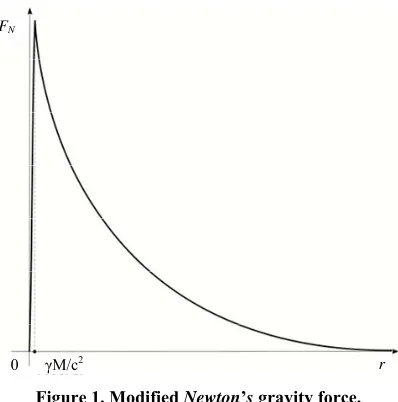
[image:6.595.324.523.82.283.2] [image:6.595.56.281.178.295.2]F , we can separate the four indicative domains of its field of the action (see
Figure 1). The first one is a domain of the weak action on finitely small distances. The second one is a domain
r FN
0 γM/c2
Figure 1. Modified Newton’s gravity force.
of the strong action in a neighborhood of the gravita- tional radius
2 0 and 2 0
r r rr r
M c F F
. The third one is a domain of the action on finitely large distances relative to the gravitational radius and with the rela- tively small velocities relative to the light velocity, and the fourth on finitely large distances relative to the gra- vitational radius and with velocities that are compa- rable to the light velocity. Previously separated domains of the field of the action of the modified Newton’s
gravity force e
N
F it would be desirable to compare to the fields of the action of the four so far non-unified fundamental forces (weak and strong nuclear interactions, gravity and Lorenz’s electromagnetism). Clearly, all of
these facts aforementioned could be subject of further analyses. Note at the end that a correction to Newton’s
gravity law in the form of the functional dependence
3 r rc
r e irresistibly reminding of the modified New- ton’s gravity force, and obviously wrongly called the fif-
th force, has been revealed by a reexamination of the old attraction data and careful new force measurements pre- sented in [11].
r
REFERENCES
[1] I. S. Lukačević, “Elements of the Relativity Theory,” Scientific Book, Belgrade, 1980.
[2] G. E. Tauber, “The General Einstein’s Relativity Theory,” Globe, Zagreb, 1984.
[3] Lj. T. Grujić, “Relativity and Physical Principle. Gener- alizations and Applications,” Proceedings of VI Interna- tional Conference: Physical Interpretations of Relativity Theory, London, 11-14 September 1998, pp. 134-155. [4] V. Pauli, “The Relativity Theory,” Science, Moscow, 1983. [5] L. D. Landau and E. M. Lifšic, “The Fields Theory,”
[9] D. Mihailović, “On Some Relations between Vector Ele- ments,” Publication of School of Electrical Engineering of Belgrade University, Series: Mathematics and Physics, Vol. 302-319, 1970, pp. 73-76.
[6] T. P. Anđelić, “Tensorial Calculus,” Scientific Book, Bel- grade, 1980.
[7] V. M. Villalba and W. Greiner, “Creation of Dirac Parti- cles in the Presence of a Constant Electric Field in an Anisotropic Bianchi I Universe,” Modern Physics Letters A, Vol. 17, No. 28, 2002, pp. 1883-1891.
doi:10.1142/S0217732302008289
[10] M. G. Stewart, “Precession of the Perihelion of Mercury’s Orbit,” American Journal of Physics, Vol. 73, No. 8, 2005, pp. 730-734. doi:10.1119/1.1949625
[8] S. Fedotov, “Front Dynamics for an Anisotropic Reac- tion-Diffusion Equation,” Journal of Physics A: Mathe- matical and General, Vol. 33, No. 40, 2000, pp. 7033- 7042.
[11] P. G. Bizetti, A. M. Bizetti-Sona, T. Fazzini and N. Tac- ceti, “Search for a Composition-Dependent Fifth Force,” Physical Review Letters, Vol. 62, No. 25, 1989, pp. 2901- 2904. doi:10.1103/PhysRevLett.62.2901
Appendix: The Freee Motion of
in the
Integral Space
and
2 2
.cos w
r d k
(57) Let us start with the Euler-Lagrange equations
Let the polar extension and the polar angle r be intensities of and an angle between the position vector and the polar axis passing through the origin and the perihelial point, respectively. Then, since
, where r
. r
p
2 const
S r S r v is the so-called
sector velocity vector, it follows from the condition (57) that the motion is the plane one
0
and S c. As
ds 2 dr
2r2
d
2 then we obtain finally from (5), (10) and (57) that
0,w
w d x
d (52)
where
,
w w
e d x d x k
(53)
as the condition for the action (12) to be stationary. The geodesic Equations (13) are explicitly obtained from it in a known way. If spatial co-ordinates are spherical ones
r, ,
, then the components of e depend only on andr , so that it follows from (52) that
2 2
2 4 2
2
1 1
dr r d
r k ,
(58)
11 0
w w
d e cd t k
(54) that just leads to the
Binet differential equation for free
motion in plane polar co-ordinates and
2 1 1 0.
d r r
(59)
33 0,
w w
d e d
k
(55)
The solution r0rcos, where 0 is the perihelial
distance, to this differential equation, defines a straight- line in plane polar co-ordinates.
r that leads to