Munich Personal RePEc Archive
Compromise and Coordination: An
Experimental Study
He, Simin and Wu, Jiabin
Shanghai University of Finance and Economics, University of Oregon
2018
Compromise and Coordination:
An Experimental Study
*
Simin He
†and Jiabin Wu
‡February 19, 2018
Abstract
This paper experimentally studies the role of a compromise option in a repeated battle-of-the-sexes game. We find that in a random-matching environment, compro-mise serves as an effective focal point and facilitates coordination, but fails to improve
efficiency. However, in a fixed-partnership environment, compromise deters subjects
from learning to play alternation, a more efficient but also more complex strategy. As a
result, compromise hurts efficiency in the long-run by allowing subjects to coordinate
on the less efficient outcome. We explore various behavioral mechanisms and suggest
that people may fail to use an equal and efficient strategy if such a strategy is complex.
Keywords: Compromise, Battle-of-the-Sexes, Repeated games, Behavioral game theory, Experimental economics.
JEL codes:C72, C92.
*We thank Yan Chen, Soo Hong Chew, Boyu Zhang and participants of the 2017 Beijing Normal University
Conference of Experimental Economics, the 2017 Nanjing International Conference on Game Theory, the 2018 ESA Asia-Pacific Meeting, and seminar participants at the City University of Hong Kong for their helpful comments and suggestions.
†School of Economics and Key Laboratory of Mathematical Economics, Shanghai University of Finance
and Economics, 111 Wuchuan Rd, 200433 Shanghai, China. E-mail: [email protected].
‡Department of Economics, University of Oregon, 515 PLC 1285 University of Oregon, Eugene, OR, USA
1 Introduction
Coordination problems are prevalent in economics and coordination is especially hard to achieve when there exist conflicts of interests. When such conflicts are difficult to resolve
given the available options, people may seek for compromise options. For example, a new couple who have different tastes for food may go to a restaurant that is not necessarily
any of their favorite but definitely acceptable for their first date. Merging firms who previously adopted different technology standards may employ a new technology that
does not require costly adjustments from any of them. Political parties with different
agendas may seek for policies in the middle ground in order to form the majority in the parliament. Foreign ministers may thrash out a formula that is acceptable across different
countries.
A compromise option naturally serves as a focal point (Schelling (1960)) for coordina-tion.1 First, it alleviates conflicts of interests. By coordinating on a compromise option, people can effectively avoid coordination failures and no one runs the risk of living with
their least favorite options. Second, it features more equal payoffs across different parties.
Hence, it is potentially favored by fair-minded players. The focality of a compromise option is found to be very effective in short-term interactions. Recently, Jackson and Xing
(2014) experimentally study a variant of a battle-of-the-sexes game featuring two equi-libria with highly asymmetric payoffs and another equilibrium with symmetric payoffs
but a slightly lower total payoff. They find that the majority of the subjects choose to
play the one with symmetric and inefficient outcome in one-shot interaction, even though
there are variations across cultures. In a more recent laboratory experiment, Bett et al. (2016) find that subjects tend to choose a symmetric but strictly dominated option to avoid coordination failure in a one-shot battle-of-the-sexes game with a third option.
While a compromise option may serve as an effective coordination device in the short
run, it is unknown how the presence of it may affect people’s decisions in the long run.
Coordination games in repeated interactions distinguish themselves from the ones in one-shot interactions, as people can rely on past interactions as their coordination device.2 Therefore, the effect of compromise options in such settings become naturally more
complicated. Would a compromise option retain its focality in repeated interactions?
1See Crawford and Haller (1990), Mehta et al. (1994) and Crawford et al. (2008) for studies on focal
points in coordination games.
2See Crawford and Haller (1990), Blume and Gneezy (2000), Lau and Mui (2008) for studies on how past
Would it help people to coordinate better or worse? Would people achieve a higher or lower long-run payoff? To our limited knowledge, few papers have investigated these
questions in the literature. The current paper serves as an attempt.
We employ a two by two experimental design: 1) Subjects repeatedly play 30 rounds of either a standard 2×2 battle-of-the-sexes game or a 3×3 variant of the game with an additional compromise option, which is similar to the one studied in Jackson and Xing (2014). There are two highly asymmetric pure strategy Nash equilibria and one symmetric but less efficient pure strategy Nash equilibrium. 2) At the beginning of the
experiment, subjects are permanently assigned to either a group of six, in which the members are randomly matched in pairs in each round (random matching), or to a group of two (fixed matching) in which the same persons are matched in each round. The comparison between the two games allows us to investigate how the compromise option would affect the subjects’ behavior; the comparison between the two matching settings
enables us to understand the role of compromise in a stranger environment and in a fixed-partnership environment, respectively.
We first find that under the random matching setting, most groups fail to coordinate better than chance in the 2×2 game. On the contrary, most groups choose to coordinate on the compromise option in the 3×3 game. This result demonstrates that the compromise option serves as a focal point in repeated interactions if people cannot form stable partner-ships. However, we do not find significant improvement in terms of average payoffwhen
the compromise option is available because those who fail to compromise earn a relatively low payoffthat offsets the payoffadvantage gained by the compromisers.
Second, we find that under the fixed matching setting, a majority of the groups learn to coordinate on a pattern of alternating between the two asymmetric pure Nash equilibria in the 2×2 game. This result confirms both the theoretical and experimental literature on alternating behavior in repeated games (see Bhaskar 2000, Lau and Mui 2008, Lau and Mui 2012, Kuzmics et al. 2014, Cason et al. 2013, Duffy et al. 2017, Romero and Zhang
2017, among many others). On the other hand, a mix of alternation and coordinating on the compromise option is observed in the 3×3 game. There is no significant difference
between the coordination rates across the two games. However, the payoff earned by
the subjects in the 3×3 game is significantly lower than that in the 2×2 game because coordinating on the compromise option is less efficient than alternation. To summarize,
seem to be short-sighted, compromise too early and give up long-term gains.
To further understand the rationale behind the main findings in the fixed matching setting, we explore several possible mechanisms. First, we confirm that the compromise option can not survive under several well-known equilibrium selection criteria such as risk-dominance, payoff-dominance (Harsanyi and Selten 1988) and the limiting quantal
response equilibrium (McKelvey and Palfrey 1995). Second, it is reasonable to assume that the more risk-averse subjects may tend to settle on a “safer” choice (compromise). However, by eliciting subjects’ risk-attitudes, we find that in the 3×3 game with fixed matching, the risk-attitudes of those who alternate are not significantly different from the compromisers.
Third, although being efficient, alternation arguably has a higher demand on subjects’
cognitive load than compromise. Therefore, there exists a trade-offbetween efficiency
and simplicity and the subjects who settle on the inefficient compromise strategy tend
to favor the latter. Our results thus share some similarities with Luhan et al. (2017) who study bargaining games and find that when a payoff-focal outcome requires complicated
coordination scheme, bargainers tend to settle on simpler and inefficient strategy.
The paper is organized as follows. Section 2 introduces the experimental design and procedure. Section 3 provides the results and tests the hypotheses. Section 4 explores the plausible behavioral mechanism behind the results. Section 5 concludes.
2 Experimental Design,Procedures and Hypotheses
2.1 Treatment design
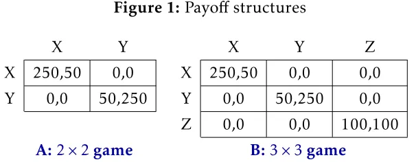
In the experiment, we implement the payoffmatrices of Figure 1. Payoffs are presented in
experimental currency. Figure 1A presents the payoffs of the specific 2×2
Battle-of-the-Sexes game and Figure 1B presents the 3×3 Battle-of-the-Sexes game with a compromise option. In both games, we keep the payoffs under actionsX andY constant. Both players
always receive zero payoffs if they choose differently. The row player prefers coordinating
on (X, X) and the column player prefers coordinating on (Y , Y). For the 3×3 game, an additional actionZis added to the 2×2 game, and both players receive an equal payoffof
100 if both chooseZ. Note that (Z, Z) is the only outcome that yields the same payofffor
both players, yet the total payoffs of (Z, Z) is lower than that of (X, X) or (Y , Y). Thus we
call this option a “compromise”, as it yields a fair outcome with an efficiency loss.
To investigate the effect of the compromise option, we first vary the game subjects play
Figure 1:Payoffstructures
X Y X Y Z
X 250,50 0,0 X 250,50 0,0 0,0 Y 0,0 50,250 Y 0,0 50,250 0,0
Z 0,0 0,0 100,100
A:2×2game B:3×3game
game in Figure 2B. Before two players are matched to play one of the two games, they are informed about their preferences. Exactly one of them has the preference of the row player, and the other has the preference of the column player. The preference of each subject is kept fixed during the entire experiment.
To see how partnership interacts with the effect of the compromise option, we also vary
the matching protocols. In a repeated play of 30 rounds, subjects are either in a random matching or a fixed matching condition. In the random matching condition, subjects are assigned in a fixed group of six. Half of the group are given the preference of the row player and the other half are given the preference of the column one. In each round, the row players and column players from the same matching group are randomly matched into pairs to play one of the games. Thus, subjects cannot form a long-term partnership with any of the players in their matching group, as they would not be able to identify each other. In the fixed matching condition, subjects are in a group of two. Similarly, one either has the preference of the row player or the column one. In contrast to the random matching condition, subjects in this condition naturally form a long-term partnership and can rely on past interactions to build future strategies. At the end of each round, each subject receives feedback about the action of her opponent and her own payoff. In order to
minimize group effect, subjects are not provided with the decisions of the entire group in
the random matching condition.
Each subject participates in only one of the treatments: one plays the 2×2 or the 3×3 game, either under random matching or fixed matching. This gives us a 2×2 between-subject design. Table 1 summarizes the treatments.
Table 1: Treatments overview
Random matching Fixed matching
2×2 game R-2 F-2
3×3 game R-3 F-3
Notes: Each cell displays the abbreviation of each treatment.
aversion. Overall, a higher number in the gamble choice task indicates a higher level of risk aversion. The details of the risk-elicitation task are provided in Appendix B.
2.2 Procedures
The experiment was conducted at the Shanghai University of Finance and Economics. Chinese subjects were recruited from the subjects pool of the Economic Lab. We ran 9 sessions in total, treatments were randomized at the session level. In each session, we ran two different treatments. For each treatment, we ran 4 or 5 sessions. We had 10
or 11 independent matching groups under random matching, and 20 or 21 matching groups under fixed matching. In total 208 subjects were recruited, most of whom were undergraduate students from various fields of studies. Table 2 presents the number of subjects, the number of independent matching groups and the number of sessions in each treatment.
Table 2: Summary of subjects
Treatments No. of subjects No. of groups No. of sessions
R-2 60 10 4
R-3 66 11 5
F-2 42 21 4
F-3 40 20 5
Total 208 62 9
The experiment was computerized using z-Tree and was conducted in Chinese.3 Upon arrival, subjects were randomly assigned a card indicating their table number and were seated in the corresponding cubicle. Before the experiment started, subjects read and signed a consent letter to agree to participate in the experiment. All instructions were
[image:7.612.131.483.489.610.2]displayed on their computer screens. Control questions were conducted to check their understanding of the instructions. The same experimenters were always presented during all the experimental sessions.
After finishing the experiment, subjects received their earnings in cash privately. Average earnings were ¥45 (equivalent to around 7 US dollars). Each session lasted between 40 to 60 minutes.
2.3 Hypotheses
We are interested in testing three hypotheses in the experiment. First of all, we expect that under random matching, the compromise option serves as an effective focal point for
coordination as found in the one-shot experiments in the literature such as Jackson and Xing (2014) and Bett et al. (2016). In addition, reducing coordination failures should also help to improve efficiency, as only coordination yields positive payoffs.
Hypothesis 1. Under random matching, compromise option improves coordination and
efficiency.
Second, we expect that under fixed matching, subjects are able to learn an efficiency
strategy in the 2×2 game, which involves alternation between the two pure Nash equi-libria. Such a strategy has been proven to be supported in subgame perfect equilibria in repeated games.4 We also expect that whenever the compromise option is available, it may deter subjects from learning the more sophisticated strategy of alternation given that the compromise option is much simpler and that it results in instant coordination success. Note that alternating between the two pure Nash equilibria in the 2×2 game yields an average payoffof 150, while the compromise option in the 3×3 game gives
each subject 100 in each round. Therefore, although introducing the compromise option may not change the rate of coordination (some subjects may switch from coordinating on alternation to coordinating on compromise), it can lower subjects’ payoffs.
Hypothesis 2. Under fixed matching, compromise option does not reduce the rate of
coordination, but hurts efficiency.
Third, we wish to understand the difference between the two matching protocols.
Con-trasting to fixed matching, random matching effectively resembles a stranger environment
in which subjects cannot form long-run partnerships and consequently are unable to learn more sophisticated strategies like alternation as in the case of fixed matching. Therefore, we expect that subjects can coordinate more successfully on better equilibria and earn a higher payoffunder fixed matching than under random matching.
Hypothesis 3. In both games, fixed matching weakly improves efficiency.
3 Results
3.1 Behavior in the
2
×
2
Battle-of-the-Sexes game
In the 2×2 Battle-of-the-Sexes game with random matching treatment (R-2), each subject meets one of the subjects in the matching group in every new round to play the game. In the stage game, there are two asymmetric pure strategy Nash equilibria with reversed payoffs for the two players, (X, X) and (Y , Y). Most of the ten matching groups fail to
converge to any of the two asymmetric Nash equilibria or any other coordination pattern.5 This result is not surprising as subjects have no obvious ways to coordinate on one of the two asymmetric equilibria. In a one-shot Battle-of-the-Sexes, standard theory predicts that subjects will use a mixed strategy. In the mixed strategy equilibrium, subjects choose the action corresponding to their favorite outcomes with a frequency of 0.83 and the other action with a rate of 0.17.6 However, in our experiment, subjects choose the former action with a rate of 0.65, which is well below the prediction (sign-rank test,p <0.01). Moreover, this rate is also well above half (sign-rank test,p <0.01), suggesting that the subjects are not using a naive randomizing strategy either.
This result serves as a benchmark of our experiment. It shows that without the possibility of forming long-run partnership or having the compromise option, subjects cannot coordinate better than chance in a Battle-of-the-Sexes game.
5The coordination rate over time in each matching group is shown in Figure 7 in Appendix C. As can be
seen, only group 2 exhibits a pattern to coordinate better over time, this might be caused by a relatively the small group size (6 subjects in each group) so that subjects are able to converge to one of the two asymmetric equilibria.
60.83 = 250
Result 1. In R-2, subjects use a mixed strategy as there is no other effective ways of achieving coordination success.
(X,
X)
(X,
Y)
(Y
,X)
(Y
,Y)
0 10 20 30 0 10 20 30
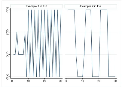
[image:10.612.204.407.127.272.2]Example 1 in F-2 Example 2 in F-2
Figure 2: Examples of behavior patterns in F-2. The x-axis is the round
number. The y-axis is the outcome distribution, in the order of (X, X),
(X, Y), (Y , X) and (Y , Y) from bottom to top.
In the Battle-of-the-Sexes game with fixed matching treatment (F-2), there exhibits a very different behavior pattern compared with that in R-2. Most of the pairs (16 out
of 21) use an alternating strategy to maximize both coordination rate and total payoffs.7
In the alternating strategy, two opponents with different preferences alternate between
each of their favorite outcomes. Two examples of such alternating strategies are shown in Figure 2. As can be seen in the left panel of Figure 2, after about 10 rounds, two players alternate between their favorite outcomes every round. By contrast, in the right panel of Figure 2, after about 5 rounds, two player alternate between their favorite outcomes by every multiple rounds. These examples suggest that subjects are not only able to use an alternating strategy, but can use it in a more complex manner. These results confirm the experimental findings of alternating strategies in repeated Battle-of-the-Sexes game (e.g. Cason et al. 2013, Duffy et al. 2017).
The advantage of the alternating strategy is twofold: First, it yields the highest total payoffthat can be achieved in such a repeated-game setting; second, it gives each player
an equal payoffonce the alternating pattern is established. This treatment therefore shows
how long-run partnership solves the coordination problem.
7Among the other five pairs, three fail to coordinate, two converge to one of the two asymmetric equilibria.
Result 2. In F-2, subjects use an alternating strategy to achieve coordination success.
3.2 Behavior in the
3
×
3
game with the compromise option
In the treatment of 3×3 Battle-of-the-Sexes game with compromise option and under random matching (R-3), in the stage game there are two asymmetric pure strategy equilib-ria (X, X) and (Y , Y) and one symmetric pure strategy Nash equilibrium (Z, Z). Among the eleven matching groups, nine groups converge to playing the symmetric equilibrium while the other two groups fail to do so.8
This result suggests that subjects rely on the compromise option to solve the coordi-nation problem otherwise presented in the 2×2 Battle-of-the-Sexes game. They quickly learn to use the compromise option exclusively and abandon using the other two actions. This provides clear evidence that among the three equilibria the symmetric one stands out as the focal point. This finding confirms and further strengthens the experimental findings of Jackson and Xing (2014) and Bett et al. (2016), as they only find in a one-shot setup that the symmetric but less efficient equilibrium is most often selected.
Result 3. In R-3, subjects use the compromise option to achieve coordination success.
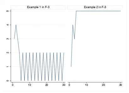
In the treatment of 3×3 game with the compromise option and under fixed matching (F-3), there exists a distinct behavior pattern compared with that in R-3. While many of the pairs (9 out of 20) use a similar alternating strategy as in F-2, a significant number of pairs (7 out of 20) converge to the symmetric equilibrium.9
This result is intriguing. Subjects fall into two distinct behavior patterns: As shown in the left panel of Figure 3, in the alternating pattern subjects play the game as if the compromise option is not presented; as displayed in the right panel of Figure 3, in the compromise pattern subjects play the game in a similar manner as in R-3.
8The compromise rate over time in each matching group is shown in Figure 8 in Appendix C. As can be
seen, only group 7 and group 16 fail to exhibit a pattern of converging to compromise over time. Sign-rank tests reports that the compromise rates in the last 15 rounds of these nine groups are not statistically different
from 0.95 at a 10 percent level.
9Among the other four pairs, three fail to converge to any pattern, and one group converges to a
0
1
2
3
4
5
0 10 20 30 0 10 20 30
[image:12.612.204.409.70.219.2]Example 1 in F-3 Example 2 in F-3
Figure 3: Examples of behavior patterns in F-3. The x-axis is the round
number. The y-axis is the outcome distribution, and number 0-5 indi-cates (X, X), (X, Y) or (Y , X), (Y , Y), (X, Z) or (Z, X), (Y , Z) or (Z, Y), and (Z, Z) respectively, from bottom to top.
Compared with R-3, the focality of the compromise option is diminished in F-3. Yet, compared with F-2, its focality still persists and partially crowds out the use of the alternating strategy.
Given that subjects fall into two categories according to the strategies they use, it is natural to ask which strategy actually gives a higher payoff. Subjects earn 130 or 92
respectively, when using the alternation or the compromise strategy (Mann-Whitney test,
p <0.001, using group level data as per observation).10 That is, alternation yields a higher
return than compromise.
Result 4. In F-3, subjects either use the alternating strategy or the compromise option to
achieve coordination success.
3.3 The e
ff
ect of compromise option on coordination
In this section we move to analysis at the treatment level. First, we investigate the effect of
compromise option on coordination. Figure 4 shows the average coordination rate in each treatment. It can be seen that while the overall coordination rate is 0.53 in treatment R-2, it is much higher in the other three treatments (0.75 in R-3, 0.80 in F-2 and 0.80 in F-3). Mann-Whitney tests show that the coordination rate in R-2 is significantly lower than the other three treatments (p <0.05), while the other three are not statistically different.
Figure 4: All-rounds verage coordination rate by treatment.
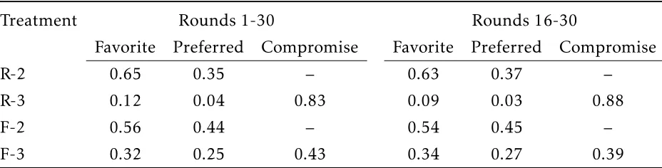
How often do subjects use the compromise option? As is shown in Table 3, under random matching, subjects use the compromise option 83% of the time overall, and this rate is increased to 88% in the last 15 rounds. This observation suggests that subjects learn to use the compromise option most of the time to avoid coordination failure. Under fixed matching, subjects use the compromise option 43% of the time overall, and 39% of the time in the last 15 rounds. Although this option is not as frequently used as in random matching, it remains the most attractive option among the three. In treatments with the 2×2 game, subjects prevalently alternate between actionsX andY, resulting in a balanced choice distribution.
Table 3: Choice distribution in each treatment
Treatment Rounds 1-30 Rounds 16-30
Favorite Preferred Compromise Favorite Preferred Compromise
R-2 0.65 0.35 – 0.63 0.37 –
R-3 0.12 0.04 0.83 0.09 0.03 0.88
F-2 0.56 0.44 – 0.54 0.45 –
F-3 0.32 0.25 0.43 0.34 0.27 0.39
[image:13.612.78.542.547.665.2]Result 5. Under random matching, the compromise option serves as a focal point and facili-tates coordination. Under fixed matching, the compromise option partially crowds out the use of the alternating strategy and induces the use of compromise as a coordination strategy.
Overall, the effect of compromise option depends on the matching protocol. Under
random matching, it is evident that compromise option largely improves coordination. The mechanism is that compromise option stands out among other actions and becomes the focal point. By choosing to compromise, the coordination problem is largely resolved. This supports Hypothesis 1 in terms of coordination. By contrast, under fixed matching, compromise option partially crowds out the use of the alternating strategy. Yet, coordina-tion failure still exists in some groups. As a result, the overall coordinacoordina-tion remains intact. This supports Hypothesis 2 in terms of coordination.
3.4 The e
ff
ect of compromise option on e
ffi
ciency
In this section we investigate the effect of compromise option on efficiency. In both games,
the maximal efficiency is achieved at one of the asymmetric equilibria, and is a constant.
Therefore, we can simply measure efficiency by the average payoffs of the subjects in all
treatments.11
Figure 5 shows the all-rounds average individual payoffs in each treatment. Under
random matching, subjects in R-2 earn 79.3 on average, while subjects in R-3 earn 76.0 on average (Mann-Whitney test,p= 0.832). Under fixed matching, subjects in F-2 receive a significantly higher payoffs than subjects in F-3 (120.7 versus 101.4, Mann-Whitney test,
p <0.05). These results suggest that the effect of compromise on efficiency are neutral
at its best: Though imposing no effect under random matching, it hurts efficiency under
fixed matching.
What are the underlying mechanism for such an neutral or even negative effect? Since
subjects in each treatment adopt different strategies over time, we turn to look at the
average payoffs for each type of the strategies. According to the group level analysis in
section 3.1 and 3.2, we group strategies into three categories. First, we call the most popular strategy in F-2 the “alternation” strategy, with which a pair of subjects alternate between achieving each of their favorite outcomes. Second, we call the most popular strategy in R-3 the “compromise” strategy, simply referring that a pair of subjects compromise and achieve the symmetric outcome. Third, we call the strategy that converging to one of the
asymmetric equilibria as the “asymmetric” strategy, though this only occurred very few times in the entire experiment. Finally, in each treatment there are always some groups that fail to converge to any of these successful strategies, which is referred as “none”.12
Figure 5: All-rounds average payoffs by treatment.
Table 4: Payoffs by type of strategy in each treatment
Treatment Rounds 16-30
Alternation Compromise Asymmetric None
R-2 – – 127 (n=1) 81 (n=9)
R-3 – 95 (n=9) – 32 (n=2)
F-2 145 (n=16) – 105 (n=2) 60 (n=3)
F-3 147 (n=9) 99 (n=7) – 53 (n=4)
Notes:“alternation” means that subjects alternate between each of their favorite and least favorite equilib-rium, “compromise” means that subjects use the compromise option, “asymmetric” means that subjects converge to play one of the asymmetric equilibria, and “none” means that subjects do not fall into the any of the first three categories. Each cell displays the rate of each action, and in the parenthesis are the number of matching groups or pairs that use the strategy.
Table 4 provides the average payoffs by the type of the strategy in each treatment.
Since we focus on the payoffs once the strategy is already used stably, we only use the data
12We call a strategy unsuccessful if in the last 10 rounds, a group or a pair of subjects fail to match their
in rounds 16-30. As can be seen from Table 4, the earnings under each type of strategy tend to be similar across treatment. For example, subjects earn slightly lower than 150 if they use the “alternation” strategy, while they earn slightly lower than 100 if they use the “compromise” strategy. Payoffs are below 150 (the mean of 50 and 250) for subjects
playing the “asymmetric” strategy as some of them sometimes deviate from the pattern. Finally, the earnings are much lower for subjects who fail to use any successful strategy to coordinate.
Under random matching, we can see from Table 4 that although the compromise option allows groups of subjects to use the “compromise” strategy, the payoffgains are not large
(from 81 under “none” in R-2 to 95 under “compromise” in R-3). Moreover, subjects who fail to use the “compromise strategy” in R-3 earn much less than subjects in R-2. As a result, there is no difference in the overall payoffs across the two treatments. Under fixed
matching, comparing F-3 and F-2, the most critical change is that the compromise option moves about half of the groups who would have used the “alternation” strategy otherwise to the use of the “compromise” strategy. This also leads to a significant payoffdrop (from
147 to 99).
Result 6. Under random matching, the compromise option overall has no effect on subjects’
average payoff. Under fixed matching, the compromise option lower subjects’ average payoff.
In sum, Result 6 does not provide supports for Hypothesis 1 which predicts a positive role of the compromise option in increasing the subjects’ payoffs. However, it does support
Hypothesis 2 in terms of efficiency.
Finally, we also find that when playing the same game, subjects always earn more under fixed matching than under random matching. In the 2×2 game, 79.3 under random matching is lower than 120.7 under fixed matching (Mann-Whitney test,p <0.01). In the 3×3 game, 76.0 under random matching is also lower than 101.4 under fixed matching (Mann-Whitney test,p <0.05). This result indicates that fixed partnership helps subjects learn more quickly on using the efficient strategy. We will talk about the pace of learning
in greater details in the next section.
Result 7. Subjects earn more under fixed matching than random matching.
3.5 Learning
[image:17.612.164.449.380.585.2]Although both games are simple, subjects may have to learn how to use the best strategies given others’ strategies and how their strategies are dependent on the past history. In this section, we briefly investigate whether there is learning effect.
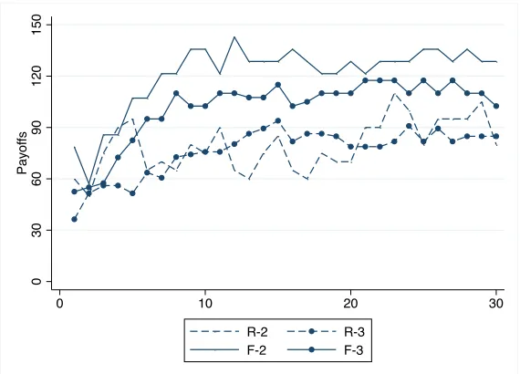
Figure 6 shows the average payoffs over rounds in each treatment. This is the best
measure for learning, as subjects are expected to earn more if they learn to use better strategies over time. As can be seen in this figure, subjects indeed earn more over time in all the treatments. Moreover, the increasing pattern is particularly strong in treatments F-2 and F-3, suggesting that subjects tend to learn more quickly under fixed matching than under random matching. This is intuitive as fixed matching allows subjects to learn the strategies of their partners in every single round. In the first few rounds, there is no obvious payoffdifference across treatments. After that, F-2 yields a higher earning pattern
than F-3, and both F-2 and F-3 yield a higher earning pattern than R-2 and R-3. This provides an explanation from a dynamic aspect for why fixed matching yields a higher payoffs in both games.
0
30
60
90
120
150
Pa
yo
ff
s
0 10 20 30
R-2 R-3
F-2 F-3
Figure 6: Average payoffs over rounds.
Result 8. There is clear evidence of learning, and the pace of learning is faster under fixed
Result 8 provides further supports for Hypothesis 3. The ability to learn under fixed matching helps subjects to achieve higher payoffs.
Next, we compare the pace of learning for subjects who use different strategies in
[image:18.612.127.498.266.324.2]treatment F-3.13 Table 5 shows the mean number of rounds before subjects converge to using either the alternation or the compromise strategy. As can be seen from the table, it takes longer for the alternators to learn their strategy than the compromisers (6.44 rounds versus 3.86 rounds,p <0.1, two-sided Mann-Whitney test), suggesting that alternation is a more complex strategy.
Table 5: Comparison of converging pace in F-3
Rounds before converging Alternation Compromise Differences
Mean rounds 6.44 3.86 2.58
SD 2.74 4.49 p= 0.083
Notes: Mann-Whitney tests are performed using pair level data.
4 Discussions
The alternation strategy payoff-dominates the compromise option, yet a significant
num-ber of subjects coordinate on the compromise option instead of alternation when the compromise option is available under fixed matching. This is in contrast to the prevalent use of alternation when compromise is unavailable. Hence, the compromise option must be associated with certain appealing features to some of the subjects. In this section, we investigate such an issue.
4.1 Equilibrium selection criteria
We first investigate whether (Z, Z) satisfies the two most well-known equilibrium selection criteria for coordination games, risk-dominance and payoff-dominance, proposed by
Harsanyi and Selten (1988).
(Z, Z) is not payoff-dominant given that switching from either (X, X) or (Y , Y) to (Z, Z)
is not a Pareto improvement.
13In F-3 subjects split into using two types of strategies, while in the other treatments subjects use at most
Harsanyi and Selten (1988) define the risk-dominant equilibrium in a 2×2 coordination game as the Nash equilibrium associated with the highest deviation lost. It implies that the more uncertainty players have about their opponents’ strategies, the more likely they will choose the strategies corresponding to the risk dominant equilibrium. Risk-dominance has been proved to be robust to incomplete information (Carlsson and van Damme 1993 and Kajii and S. 1997) and evolutionary learning (Kandori et al. 1993 and Young 1993).
In coordination games with more than two strategies, half-dominance may serve as proper generation of Harsanyi and Selten’s idea (see Morris et al. 1995, Sandholm 2001 and Oyama et al. 2015).14 A strategy profile (s1, s2) is half-dominant ifsi is the unique best
response for playeri as long as playerj playssj with at least 12 probability, wherei ,j and
i, j∈ {1,2}. In Appendix A, we verify that (Z, Z) is not a half-dominant equilibrium in our 3×3 game given any degrees of risk-aversion for the two players.
In sum, both payoff-dominance and risk-dominance cannot explain why some pairs of
subjects in F-3 converge to (Z, Z).
Next, we consider the concept of quantal response equilibrium (QRE) proposed by McKelvey and Palfrey (1995). QRE captures the idea that boundedly rational players do not always choose best responses. Instead, they follow some probabilistic choice procedure and they also believe that their opponents behave in the same way. The most common specification of QRE is the logit equilibrium in which a single parameterλcaptures the sophistication level of the players. Whenλ= 0, players have no information about the game and they choose uniformly randomly over all the pure strategies. Whenλ→+∞, the players are sufficiently sophisticated and are able to choose best responses. QRE has been
widely adopted in the literature to explain experimental data. See for example, Anderson et al. (1998), Anderson et al. (2001), Capra et al. (1999), Goeree and Holt (2000), Goeree and Holt (2001), Goeree et al. (2002), Yi (2005), Choi et al. (2012), among many others.
McKelvey and Palfrey (1995) suggest an equilibrium selection criterion by tracing the branch of the logit equilibrium correspondence starting from the centroid of the strategy simplex (the only QRE when λ = 0) until it reaches the terminus asλ → +∞. They call the selected equilibrium thelimitingQRE. The idea of limiting QRE is that as players become more sophisticated (λincreases), they are able to coordinate on a certain equilibrium. Subjects gaining experience and becoming more sophisticated through repeated interactions has been observed in many of the above mentioned experimental works.
Recently, Zhang and Hofbauer (2016) and Zhang (2016) systematically study the equilibrium selection problem in normal form games based on limiting QRE. In particular, they find that in 2×2 coordination games, the limiting QRE may not coincide with the risk-dominant equilibrium.
In Appendix A, we use the approximation method by Zhang and Hofbauer (2016) and show that (Z, Z) is not the limiting QRE in our 3×3 game as long as the players are not sufficiently risk-averse. For example, suppose that the players are equipped with the CRRA
utility function with parameterθ, whereθmeasures the degree of risk aversion.15 When
θ <1.35, (Z, Z) is not the limiting QRE. Hence, if subjects become more sophisticated
during the experiment, they would not tend to coordinate on (Z, Z).
Finally, we consider the size of the basin of attraction of strategyZ(sizeBAZ), a simple statistic of measuring the trade-offbetween alternation and compromise. In the
experimen-tal literature, basin of attraction has been used to determine the likelihood of choosing to cooperate in repeated prisoner’s dilemmas (Dal B ´o and Guillaume 2011 and Embrey et al. 2017) and of choosing to coordinate on the payff-dominant convention in coordination
games (Belloc et al. 2017). Assume that subjects only consider two extreme strategies: alternation and compromise, thensizeBAZis the probability that a subject must assign to the other subject playingZ so that she is indifferent between alternation and compromise.
We have sizeBAZ = 100+0.5100∗(150+50) = 0.4, which is smaller than the basin of attraction corresponding to alternation, 1−0.4 = 0.6, implying that the subjects are less likely to choose to compromise when facing strategic uncertainty. Note that if the payoffassociated
with (Z, Z) increases,sizeBAZenlarges, implying that subjects may be more likely to choose to compromise. We leave interested reader to explore how parameters change affects play
in the 3×3 game.
4.2 Risk attitudes
Risk attitude could be one of the reasons for why some pairs converge to the symmetric equilibrium. If at least one of the subject in a pair is very risk averse, she might not want to establish an “alternating” pattern, as there is a risk of not receiving her own favorite outcome in the future periods.
In addition, from the analysis of the limiting QRE in the previous section, we know that (Z, Z) is possible to be the limiting QRE if the subjects are sufficient risk-averse.
To assess whether risk attitude plays a role in affecting subjects’ decisions, we compare
the choices made in the risk-elicitation part of the experiment by subjects who alternate and those who compromise in treatment F-3.
Table 6: Comparison of risk attitudes in F-3
Risk elicitation Alternation Compromise Differences
Mean choice 3.78 4.36 0.58
SD 1.52 1.39 p= 0.28
Notes: higher choice indicates higher level of risk-aversion. Mann-Whitney tests are performed using pair level data.
From table 6, one can observe that the compromisers are slightly more risk-averse than the alternators on average. However, the difference is not significant. Moreover, the mean
choice for the compromisers suggests that they are approximately indifferent between
Option 4 and 5, which corresponds to a parameter value of θ= 1.16 in a CRRA utility function. According to the analysis on limiting QRE in the previous section, this parameter value would not allow (Z, Z) to be the limiting QRE. Hence, we conclude that risk attitude cannot explain why some pairs compromise.
4.3 Complexity of the strategy
Though being efficient, alternation is more complex than compromise as it requires the
two subjects to alternate between two different outcomes instead of choosing the same
action every round. Hence, it arguably requires a higher cognitive load than compromise does. We therefore argue that there is a trade-offbetween the efficiency and the simplicity
(complexity) of each available strategies. Some subjects may settle for the less efficient
strategy for its simplicity. Luhan et al. (2017) also find that in bargaining games, many subjects tend to settle on equal and inefficient payoffs if it is more complex to achieve
equal and efficient payoffs.
So far, this seems to be the most plausible explanation for why many of the subjects settle on the inefficient compromise strategy. It suggests that in similar settings like the
one we consider in this paper, one cannot expect subjects to use an equal and efficient
5 Conclusion
In this paper, we investigated how a compromise option affects play in a Battle-of-the-sexes
game under random matching (repeated one-shot game) and under fixed matching (re-peated games). Experimentally, we found that the effectiveness of the compromise option
depended crucially on the matching protocol. Under random matching, the inclusion of the compromise option affected play drastically, as most subjects tended to use the
compromise option to avoid coordination failure otherwise existed without such an option. In contrast, under fixed matching, compromise option partially crowded out subjects from the use of the alternation strategy and led to a lower payoffas many subjects used
compromise as a way to coordinate.
This study is the first attempt to the understanding of the role of focal points in repeated interactions. Different from short-term interactions, players can rely on additional
mechanisms to achieve coordination in repeated interactions. Yet, the role of focal points is unclear. Our findings provide evidence that compromise option retains its salience in repeated games because of its symmetry and simplicity, though less salient compared to in one-shot games. Our results raise an important question on whether other types of focal points can retain their focality in repeated games.
References
Anderson, S., Goeree, J., and Holt, C. (1998). Rent seeking with bounded rationality: an anlysis of the all-pay auction. Journal of Political Economy, 106:828–853.
Anderson, S., Goeree, J., and Holt, C. (2001). Minimum effort coordination games:
stochas-tic potential and the logit equilibrium. Games and Economic Behavior, 34:177–199.
Belloc, M., Bilancini, E., Boncinelli, L., and D’Alessandro, S. (2017). A social heuristics hypothesis for the stage hunt: Fast- and slow-thinking hunters in the lab.Working paper.
Bett, Z., Poulsen, A., and Poulsen, O. (2016). The focality of dominated compromises in tacit coordination situations: Experimental evidence. Journal of Behavioral and
Experi-mental Economics, 60:29–34.
Bhaskar, V. (2000). Egalitarianism and efficiency in repeated symmetric games. Games and
Blume, A. and Gneezy, U. (2000). An experimental investigation of optimal learning in coordination games. Journal of Economic Theory, 90(1):161–172.
Capra, C., Goeree, J., Gomez, R., and Holt, C. (1999). Anomalous behavior in a travelers dilemma? American Economic Review, 89:678–690.
Carlsson, H. and van Damme, E. (1993). Global games and equilibrium selection.
Econo-metrica, 61:989–1018.
Cason, T. N., Lau, S. H. P., and Mui, V. L. (2013). Learning, teaching, and turn taking in the repeated assignment game. Economic Theory, 54:335–357.
Choi, S., Gale, D., and Kariv, S. (2012). Social learning in networks: a quantal response equilibrium analysis of experimental data. Review of Economic Design, 16:135–157.
Crawford, V. P., Gneezy, U., and Rottenstreich, Y. (2008). The Power of focal points is limited: Even minute payoffasymmetry may yield large coordination failures. American
Economic Review, 98:1443–1458.
Crawford, V. P. and Haller, H. (1990). Learning how to cooperate: Optimal play in repeated coordination games. Econometrica, 58:571–595.
Dal B ´o, P. and Guillaume, F. (2011). The evolution of cooperation in infinitely repeated games: Experimental evidence. American Economic Review, 101:411–429.
Duffy, J., Lai, E. K., and Lim, W. (2017). Coordination via correlation: an experimental
study. Economic Theory, 64:1–40.
Eckel, C. C. and Grossman, P. J. (2008). Forecasting risk attitudes: An experimental study using actual and forecast gamble choices. Journal of Economic Behavior and Organization, 68(1):1–17.
Embrey, M., Guillaume, F., and Yuksel, S. (2017). Cooperation in the finitely repeated prisoner’s dilemma. Quarterly Journal of Economics, forthcoming.
Goeree, J. and Holt, C. (2000). Asymmetric inequality aversion and noisy behavior in alternating-offer bargaining games. European Economic Review, 44:1079–1089.
Goeree, J., Holt, C., and Palfrey, T. (2002). Quantal response equilibrium and overbidding in private-value auction. Journal of Economic Theory, 104:247–272.
Goeree, J., Holt, C., and Palfrey, T. (2005). Regular quantal response equilibrium.
Experi-mental Economics, 8:347–367.
Harsanyi, J. C. and Selten, R. (1988). A General Theory of Equilibrium Selection in Games.
Cambridge: MIT Press.
Jackson, M. O. and Xing, Y. (2014). Culture-dependent strategies in coordination games.
Proceedings of the National Academy of Sciences, 111:10889–10896.
Kajii, A. and S., M. (1997). The robustness of equilibria to incomplete information.
Econometrica, 65:1283–1309.
Kandori, M., Mailath, G. J., and R., R. (1993). Learning, mutation, and long run equilibria in games. Econometrica, 61:29–56.
Kuzmics, C., Palfrey, T., and Rogers, B. W. (2014). Symmetric play in repeated allocation games. Journal of Economic Theory, 154:25–67.
Lau, S. H. P. and Mui, V. L. (2008). Using turn taking to mitigate coordination and conflict problems in the repeated Battle of the Sexes game. Theory and Decision, 65:153–183.
Lau, S. H. P. and Mui, V. L. (2012). Using turn taking to achieve intertemporal cooperation and symmetry in infinitely repeated 2×2 games. Theory and Decision, 72:167–188.
Luhan, W. J., Poulsen, A. U., and Roos, M. W. (2017). Real-time tacit bargaining, payoff
focality, and coordination complexity: Experimental evidence. Games and Economic
Behavior, 102:687–699.
McKelvey, R. and Palfrey, T. (1995). Quantal response equilibria for normal form games.
Games and Economic Behavior, 10:6–38.
Mehta, J., StarmerRobert, C., and Sugden, R. (1994). Focal points in pure coordination games: An experimental investigation. Theory and Decisions, 97:19–31.
Oyama, D., Sandholm, W. H., and Tercieux, O. (2015). Sampling Best Response Dynamics and Deterministic Equilibrium Selection. Theoretical Economics, 10:243–281.
Romero, J. and Zhang, H. (2017). Egalitarianism and turn taking in repeated coordination games. working paper.
Sandholm, W. H. (2001). Almost Global Convergence to p-Dominant Equilibrium.
Inter-national Journal of Game Theory, 30:107–116.
Schelling, T. C. (1960). The strategy of conflict (First ed.). Cambridge: Harvard University Press.
Yi, K. (2005). Quantal response equilibrium models of the ultimatum bargaining game.
Games and Economic Behavior, 51:324–348.
Young, P. (1993). The evolution of conventions. Econometrica, 61:57–84.
Zhang, B. (2016). Quantal response methods for equilibrium selection in normal form games. Journal of Mathematical Economics, 64:113–123.
Zhang, B. and Hofbauer, J. (2016). Quantal response methods for equilibrium selection in 2×2 coordination games. Games and Economic Behavior, 97:19–31.
Appendices
Appendix A: Proofs
In this appendix, we first show that (Z, Z) in our 3×3 game is not the half-dominant equilibrium.
Assume that both players are von Neumann-Morgenstern expected utility maximizers and their Bernoulli utility functions strictly increase in money.
Letsi∈ {X, Y , Z}andpi∈∆{X, Y , Z}denote a pure strategy and a mixed strategy played
by playeri, respectively, wherei ∈ {1,2}.
Definition 1. A pure strategy profile(s1, s2)is half-dominant ifUi(si, pj)> Ui(si′, pj)for anypj
satisfyingpj(sj)≥ 12, wheres′i,si,i,j,i, j∈ {1,2}.
Proof. Letp2 = 12X+ 12Z, thenU1(X, p2) = 12u1(250)> U1(Z, p2) = 12u1(100). Similarly, let
p1=12Y+12Z, thenU2(Y , p1) =12u2(250)> U2(Z, p1) = 12u2(100). Hence, we conclude that (Z, Z) violates the definition of the half-dominant equilibrium.
Next, we investigate whether (Z, Z) is the limiting QRE. For illustration purposes, we assume that both players have identical preferences over money, represented by a Bernoulli utility functionu:R→R, and they follow the same logit choice rule:
σi(si) =
eλUi(si,pj)
eλUi(X,pj)+eλUi(Y ,pj)+eλUi(Z,pj), i,j andi, j ∈ {1,2},
whereλ >0 denotes the noise level.σi(si) denotes the probability of playeri choosing si under the logic choice rule.
Definition 2. A mixed strategy profile(p1, p2)is a quantal response equilibrium (QRE) at noise
levelλifpi(si) =σi(si)forsi ∈ {X, Y}andi∈ {1,2}.16
Whenλ= 0,pi =pj = (13,13,13) is the unique QRE, which is the centriod of the strategy
space simplex. When λ= ∞, all Nash equilibria of the game are QREs. According to Theorem 6 of Zhang (2016), since logit choice rule satisfies the definition of regular quantal response function by Goeree et al. (2005), there exists a continuous path (branch) of QRE correspondences that starts at the centroid as λ = 0 and converges to one of the Nash equilibria asλ→ ∞, which defines a unique equlibrium selection called thelimitingQRE.
Proposition 2. Whenu(250) +u(50)>2u(100),(Z, Z)is not the limiting QRE.
Proof. We divide the strategy space simplex into two partsA1={(p1, p2)|p1(X) +p1(Y) +
p2(X) +p2(Y)> 43}andA2={(p1, p2)|p1(X) +p1(Y) +p2(X) +p2(Y)< 43}by the planep1(X) +
p1(Y) +p2(X) +p2(Y) = 43. The path of QRE correspondences intersects with the plane at
pi=pj= (13,13,13), the unique QRE whenλ= 0. We numerically verify that this is the only
intersection, meaning that for any otherλ >0, there is no QRE lands on the plane. This implies that asλincreases from 0, the path will enter eitherA1orA2and cannot escape from it.
We define a functionf :R×R→Rsuch thatf(x, y) = 1
1+e−x+e−y. f1>0 andf2 >0. We
can rewrite the logit choice rule as follows:
σi(X) =f(λ(Ui(X, pj)−Ui(Y , pj)), λ(Ui(X, pj)−Ui(Y , pj))),
σi(Y) =f(λ(Ui(Y , pj)−Ui(X, pj)), λ(Ui(Y , pj)−Ui(Z, pj))), i,j andi, j∈ {1,2}.
16Note that we do not specifyp
Whenλ→0+, the equations defining a QRE,pi(si) =σi(si) forsi ∈ {X, Y}andi∈ {1,2},
can be approximated as
pi(X) =σi(X) =
1
3+λ(Ui(X, pj)−Ui(Y , pj))f1+λ(Ui(X, pj)−Ui(Z, pj)))f2+O(λ
2),
pi(Y) =σi(Y) =
1
3+λ(Ui(Y , pj)−Ui(X, pj))f1+λ(Ui(Y , pj)−Ui(Z, pj))f2+O(λ
2),
fori,j andi, j∈ {1,2}.
Note that U1(X, p2) =u(250)p2(X),U1(Y , p2) =u(50)p2(Y) andU1(Z, p2) =u(100)(1−
p2(X)−p2(Y));U2(X, p1) =u(50)p1(X),U2(Y , p1) =u(250)p1(Y) andU2(Z, p1) =u(100)(1−
p1(X)−p1(Y)). We have
p1(X) +p1(Y) +p2(X) +p2(Y) = 4
3+λ((u(50) + 2u(100))p1(X) + (u(250) + 2u(100))p1(Y) +(u(250) + 2u(100))p2(X) + (u(50) + 2u(100))p2(Y)
−4u(100))f2+O(λ2) = 4
3+λ( 2
3u(250) + 2
3u(50)− 4
3u(100))f2+O(λ
2).
Hence, as long as u(250) +u(50)>2u(100), the path of QRE correspondences enter regionA1 and cannot escape. Since (Z, Z) is in regionA2, (Z, Z) cannot be the limiting
QRE.
Appendix B: Experimental Instructions
In this appendix, we provide the experimental instructions that are translated from the original Chinese version.
Instructions
Welcome to this experiment on decision-making. Please read the following instructions carefully. During the experiment, do not communicate with other participants in any means. If you have any question at any time, please raise your hand, and an experimenter will come and assist you privately. This experiment will last about one hour.
It is an anonymous experiment. Experimenters and other participants cannot link your name to your desk number, and thus will not know the identity of you or of other participants who made the specific decisions. During Part I, your earnings are denoted in points. Your earnings depend on your own choices and the choices of other participants. At the end of the experiment, your earnings will be converted to RMB at the rate: 100 points = ¥ 1. During Part II, your earnings are denoted directly in RMB currency Yuan. In addition, you receive 10 RMB show-up fee. This show-up fee is added to your earnings from Part I and Part II. Your total earnings will be paid to you in cash privately.
Part I (Treatment R-3)
In this experiment, you will stay in a group of six people. In each round, you will be randomly matched with one person in the room. The two of you are going to play a game. Each person will make a choice between A, B and C. If you and the other person make a different choice, you will both receive 0 points. If you and the other person both choose A,
you will receive 250 points and the other person will receive 50 points. If you both choose B, then you will receive 50 points and the other person will receive 250 points. If you both choose C, both of you will receive 100 points.
The possible decisions and payoffs are also shown in the following matrix. In each
cell of the matrix, the first number shows the amount of points for you, and the second number shows the amount of points for the other person.
You will play this game for 30 rounds in total. In these 30 rounds, you will be matched within your matching group of six people. You will not be matched with someone with the same preferences as you. Therefore, you will be only matched with 3 different participants
in this group. In each round, you will be re-matched to one of the 3 participants. In each round, the chance of meeting any of the three participants is one third. At the end of each round, you will learn the choice of your partner in this round. Your earnings in this experiment equal the sum of the points you earn in all of the 30 rounds plus the show-up fee. Your earnings will be converted to RMB at the rate: 100 point = ¥ 1.
Quiz
1. In each round, what is your payoffif you choose A and the other person chooses C?
2. In one round, what is your payoffif both you and the other person choose B? How about
the payoffof the other person?
4. Which of the following statements below is true? a. I will play with the same person in all the rounds. b. I will never play with the same person for more than one round. c.I might play with the same person for more than one round.
5. Suppose you are now in round 10, which statement below is true? a. I will play with the same person in the next round. b. I might play with a different person in the next round.
c.I will definitely play with a different person in the next round.
Part II
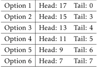
In the table below, we present six different options. You are asked to select one of the
[image:29.612.222.391.379.495.2]options. Your earnings will depend on the outcome of a fair coin toss generated by the computer. Every option shows the amount in points you earn in case a head shows up or a tail shows up. The chance of head or tail is 50% respectively. When you have made your choices, the computer will randomly decide the result of the coin toss. Please indicate which one of the six options you prefer.
Table 7:Options in the Risk-elicitation task
Option 1 Head: 17 Tail: 0 Option 2 Head: 15 Tail: 3 Option 3 Head: 13 Tail: 4 Option 4 Head: 11 Tail: 5 Option 5 Head: 9 Tail: 6 Option 6 Head: 7 Tail: 7
Appendix C: Supplemental tables and figures
0 .5 1 0 .5 1 0 .5 1
0 10 20 30 0 10 20 30
0 10 20 30 0 10 20 30
1 2 10 11
14 15 18 19
[image:30.612.136.479.83.332.2]24 27 co o rd in a ti o n ra te
Figure 7: Group-Level Data, R-2. Coordination rate over time. Notes:
X-axis is round number. Y-axis shows the coordination rate.
.2 .4 .6 .8 1 .2 .4 .6 .8 1 .2 .4 .6 .8 1
0 10 20 30
0 10 20 30 0 10 20 30 0 10 20 30
4 6 7 8
13 16 17 21
23 25 26
co mp ro mi se ra te
Figure 8: Group-Level Data, R-3. Compromise rate over time. Notes:
[image:30.612.134.478.411.663.2]1 2 3 4 1 2 3 4 1 2 3 4 1 2 3 4 1 2 3 4
0 10 20 30 0 10 20 30 0 10 20 30 0 10 20 30
0 10 20 30
31 32 33 34 35
36 37 38 121 122
123 124 125 126 127
128 201 202 203 204
205
O
u
tco
[image:31.612.135.480.74.325.2] [image:31.612.136.478.406.650.2]me
Figure 9: Group-Level Data, F-2. Outcome distribution over time.
Notes: X-axis is round number. Number 1-4 in y-axis indicates outcome (X,X), (X,Y), (Y,X), (Y,Y), respectively. 0 1 2 3 4 5 0 1 2 3 4 5 0 1 2 3 4 5 0 1 2 3 4 5
0 10 20 30 0 10 20 30 0 10 20 30 0 10 20 30 0 10 20 30
51 52 53 54 55
56 57 58 91 92
93 94 95 221 222
223 224 225 226 227
O
u
tco
me
Figure 10: Group-Level Data, F-3. Outcome distribution over time.