Munich Personal RePEc Archive
Tax Evasion and Optimal Corporate
Income Tax Rates in a Growing Economy
Hori, Takeo and Maebayashi, Noritaka and Morimoto,
Keiichi
22 December 2018
Online at
https://mpra.ub.uni-muenchen.de/90787/
Tax Evasion and Optimal Corporate Income Tax Rates
in a Growing Economy
∗
Takeo Hori
†Noritaka Maebayashi
‡Keiichi Morimoto
§December 22, 2018
Abstract
We explore how tax evasion by firms affects the growth- and welfare-maximizing rates
of corporate income tax (CIT) in an endogenous growth model with productive public
ser-vice. We show that the negative effect of CIT on growth is mitigated in the presence of tax
evasion. This increases the benefit of raising the CIT rate for public service provision. Thus,
in contrast to Barro (1990), the optimal tax rate is higher than the output elasticity of public
service. Through numerical exercises, we demonstrate that the role of tax evasion by firms
is quantitatively significant.
Keywords: corporate income tax, tax evasion, growth, welfare
∗We are grateful to Shingo Ishiguro, So Kubota, Kazutoshi Miyazawa, Ryoji Ohdoi, Makoto Saito, Daichi Shirai,
Koki Sugawara, Yuta Takahashi, Akira Yakita, and Taiyo Yoshimi for their helpful comments. We also thank the participants of the 2018 Public Economic Theory Conference, Journ´ees LAGV 2018, 2018 Australasian Meeting of Econometric Society, MUETEI workshop at Meisei University, Nagoya Macroeconomic Workshop, Economic Theory and Policy Workshop, the Macro Money Workshop at Hitotsubashi University, and the Economics Seminar at Tokyo International University. We are responsible for any remaining errors.
†Department of Industrial Engineering and Economics, School of Engineering, Tokyo Institute of Technology,
2-12-1, Ookayama, Meguro-ku, Tokyo, 152-8552, Japan. E-mail address: hori.t.ag@m.titech.ac.jp
‡Faculty of Economics and Business Administration, The University of Kitakyushu, 4-2-1, Kitagata, Kokura
Minami-ku, Kitakyushu, Fukuoka 802-8577, Japan. E-mail address: non818mn@kitakyu-u.ac.jp
§Department of Economics, Meisei University, 2-1-1, Hodokubo, Hino, Tokyo 191-8506, Japan. E-mail address:
1
Introduction
Corporate income tax (hereafter, CIT) has detrimental effects on investment by firms. Modern prevailing opinions advocate that CIT should be cut to promote economic growth. In reality,
governments in developed countries have lowered the CIT rate in recent years: The average rate of CIT in OECD countries decreased from 32.5% to 24.2% between 2000 and 2017. 1 However,
because CIT is an important tax basis for public finance, cutting the CIT rate reduces public investment in infrastructure (productive public services) and may lower the rate of economic
growth (e.g., Barro 1990).2 Therefore, setting CIT rates involves a trade-off between private investment and the provision of productive public services for economic growth, and it is an
important policy issue.
In addition, tax evasion by firms is a serious problem of CIT. There is large-scale tax evasion
in real economies. For example, in the US, the Internal Revenue Service (2016) reports about 44 billion dollars as the estimated tax gap of CIT on annual average from 2008 to 2010.3
Nonethe-less, the actual audit coverage of taxed corporations is very limited, primarily because of fiscal tightness; only 1.0% of taxed returns were examined in the US in 2016 and only 3.1% of all taxed
corporations were audited in Japan in 2015.4
One of the most general ways of tax evasion is to underdeclare income (e.g., Allingham and
Sandmo 1972). To underdeclare corporate income, firms may pretend to have lower productivity and overstate their costs. In reality, there is institutional cause for such tax evasion behavior at
the microeconomic level. The CIT systems in many countries have reduction and exemption measures; deficits of corporations can be carried forward and CITs of corporations with small
income are reduced or exempted. Such systems give corporations an incentive to underdeclare their profit intentionally by overstating cost. These are neither unusual nor insignificant at the
macroeconomic level. For example, the National Tax Agency (2016) reports that more than two-thirds of the ordinary corporations in Japan were loss corporations between 2011 and 2015 on
1
According to the policy stance of President Trump, the US government reduced the CIT rate to21%. In Japan, the government plans to cut the CIT rate to about20% gradually under some conditions.
2
In fact, CIT occupies a considerable fraction of the annual revenue of the public sector. For example, the Internal Revenue Service (2017) and the National Tax Agency (2017) report that the shares of CIT to total tax revenues were about 10% in the US in 2016 and 19% in Japan in 2015, respectively.
3Here, the “tax gap” is the “gross tax gap” in the Internal Revenue Service’s survey. This is defined as the amount
of true tax liability that is not paid voluntarily and timely. For details, see Internal Revenue Service (2016).
average. The reported losses amounted to 11.3 billion yen in 2015 and occupied a quarter of the reported total income of the corporate sector.
With these problems of CIT as motivation, this study investigates an optimal CIT policy in a growing economy with tax evasion by firms. The evaded tax payments are utilized for private
investment, while a part of the tax revenue is lost. This affects the trade-off between private investment and the provision of productive public services. We are particularly interested in how
CIT evasion by firms changes the optimal rate of CIT.
To tackle this problem, we construct a variety-expansion model of growth in which private
firms invest to earn monopolistic profits and their investments sustain economic growth. 5 A single final good is produced by using intermediate goods. Each intermediate good is produced
by a monopolistically competitive firm. Each intermediate good firm invests to enter into business and pursues monopolistic profits. CIT discourages private investment because the monopolistic
profits are subject to CIT. On the other hand, productive public services have a positive effect on the monopolistic profits of intermediate good firms. Thus, CIT has a positive effect on private
investment through productive public services financed by CIT.
In our model, facing CIT, firms have an incentive to evade tax payment by underdeclaring
their profits in the absence of a perfect tax enforcement system. Because each firm can avoid a part of tax payment, tax evasion weakens the discouraging effect of CIT on private investment.
Simultaneously, tax evasion reduces the provision of productive public services. Thus, tax eva-sion by the corporate sector affects private investment, provieva-sion of productive public services,
and economic growth.
In a tractable model, we obtain a qualitative result that both the growth- and welfare-maximizing
CIT rates are higher than the output-elasticity of public service. This is in contrast to the familiar Barro’s (1990) rule, which indicates that the tax rate should be set at the output elasticity of public
services. The mechanism behind our result is as follows. When the government raises the CIT rate, the effective CIT rate and the tax revenue rise.6 This increases the provision of productive
public services and promotes economic growth. Simultaneously, raising the CIT rate discour-ages private investment and has a detrimental effect on growth. However, this negative effect on
growth is weakened by tax evasion. This is because, in response to a tax hike, firms attempt to
5We follow Barro and Sala-´ı-Martin’s (2004) variety-expansion model.
6Here, we mean that the effective tax rate is the ratio of the actually collected CIT revenue to the true profits of
secure profits by increasing tax evasion. It alleviates the reduction in private investment and the tax base of CIT. CIT evasion generates the benefits of raising the CIT rate for the provision of
productive public services.
Next, we extend the model to obtain quantitative results. Our quantitative analyses show that
tax evasion significantly raises the optimal CIT rate. In particular, the optimal tax rate is 40% for the benchmark case, which is much higher than the standard values of the output elasticity of
public service, e.g., 10%. This optimal CIT rate in our model, at 40%, is close to that in Aghion et al. (2016) mentioned below. Besides, we decompose the difference between the optimal tax
rate and the output elasticity of public service into several parts including a part associated with the effect of CIT evasion. We find that the effect of CIT evasion occupies more than half of the
total difference between the optimal tax rate and the output elasticity of public service for a wide range of reasonable parameter values. That is, even quantitatively, the effect of CIT evasion is
the main source of the high optimal tax rate.
Related Literature
Largely, our study is part of the literature starting with Barro (1990), which explores optimal taxation in an endogenous growth model with productive public service (capital) (e.g., Futagami
et al, 1993; Glomm and Ravikumar, 1994; Turnovsky 1997).7 These studies emphasize that the growth-maximizing income tax rate equals the output elasticity of public capital and it coincides
with the welfare-maximizing one in the balanced growth path. This is the so-called Barro rule. More recent studies cast some doubts on the Barro rule. Some studies (e.g., Futagami et al.
1993; Ghosh and Roy 2004; Ag´enor 2008) show that the welfare-maximizing tax rate is lower than the growth-maximizing one (output elasticity of public capital), while other studies (e.g.,
Kalaitzidakis and Kalyvitis 2004; Chang and Chang 2015) show the opposite result.8 While these existing studies consider neither CIT nor tax evasion, our study investigates optimal taxation,
7
Some empirical studies suggest the importance of productive public expenditure for economic growth. Abiad et al. (2016) show that increases in public investment in infrastructure raise output in both the short and long run.
8
theoretically and quantitatively, incorporating CIT evasion.9
Among the existing studies of tax evasion and growth, we should refer to Chen (2003) and
Kafkalas et al. (2014). They investigate tax evasion by household-firms in Barro’s (1990) type model, in which government incurs inspection expenditure to audit taxpayers. These authors
focus on the trade-off between the government’s inspection expenditure and public investment. Chen (2003) shows that the growth-maximizing announced tax rate is higher than the output
elasticity of public service, under the assumptions that inspection expenditure is proportional to output and household-firms must incur tax evasion costs. On the other hand, Kafkalas et al.
(2014) assume that the government’s inspection expenditure is proportional to tax revenues. They show that, even with tax evasion, the growth-(and utility-) maximizing effective tax rate equals
the output elasticity of public capital, in line with Barro’s rule.
In contrast to these studies, we do not focus on the role of inspection expenditure. Therefore,
we adopt the same specification of inspection expenditure as Kafkalas et al. (2014), which does not affect Barro’s rule. Thus, we can concentrate on the role of tax evasion behavior of firms with
market power.
Although the findings on optimal tax rates from Chen (2003) and Kafkalas et al. (2014) are
interesting, there are some reservations. First, they consider tax evasion by household-firms, where the firm is the same as a household. Since there is no difference between CIT and a
household’s income tax in their models, they do not consider the role of CIT evasion. Second, they assume a competitive goods market, and therefore, ignore tax evasion associated with profit
maximization in an imperfectly competitive product market.10 Thus, although tax evasion affects the aggregate economy through the government budget in their models, these studies do not
consider the role of tax evasion in the production side directly.
Our study is also comparable to Aghion et al. (2016). They examine the relationship among
corporate taxation, growth, and welfare, focusing on corruption. Aghion et al. (2016) construct
9
Ag´enor and Neanidis (2017) show empirically that public capital affects growth through productivity and inno-vation (R&D) capacity.
10
an endogenous growth model in which public capital raises the expected returns to entrepreneurial efforts on R&D but tax revenue decreases due to the corruption of officers after tax collection.
They suggest that the relationship between CIT rate and growth is an inverted-U shape and the welfare-maximizing CIT rate is 42% in the calibrated model. However, Aghion et al. (2016) do
not consider tax evasion by firms but focus on the corruption between government and house-holds. In this study, we incorporate corporate tax evasion in an endogenous growth model and
suggest that the optimal CIT rate is as high as Aghion et al.’s (2016) estimate.
2
Model
Time is discrete and denoted by t = 0,1, · · ·. The economy is inhabited by the following four types of agents: producers of final output, producers of intermediate goods, a representative household, and government. An infinitely lived representative household has perfect foresight
and is endowed withLunit of labor. Labor moves freely across different production sectors. The number of intermediate good in periodtisNt. We assumeN0 = 1without loss of generality.
2.1
Producers of final good
A single final output is produced by perfectly competitive producers using the following technol-ogy:
Yt =AL1
−α
Y,t
∫ Nt
0
(Gtxi,t)αdi, A >0, 0< α <1, (1)
whereYtis output,LY,tis labor input in the final goods sector, andxi,tis the input of intermediate
good i. Following Barro (1990), public services,Gt, increases the productivity of output. We
take the final output as the numeraire. Although α encompasses both (i) the output elasticity of public services and (ii) the price elasticity of intermediate goods1/(1−α), we examine the former in this simple model. In the extended model (Section 5), we separate (i) and (ii). We denote the price of intermediate good i and wage rate as pi,t and wt, respectively. The profit
maximization yields
wt= (1−α)AL−Y,tα
∫ Nt
0
(Gtxi,t)αdi= (1−α)
Yt
LY,t
, (2)
pi,t =αAL1Y,t−αGαtxα
−1
Solving (2) and (3) with respect toxi,tyields the demand function for the product of firmi:
x(pi,t)≡
(1−α)Yt
wt (
αAGα t
pi,t
) 1
1−α
.
2.2
Producers of intermediate goods
2.2.1 Entry into the intermediate goods market
Each intermediate good is produced by a monopolistically competitive firm. To operate in period
t, each intermediate good firm must investηunit of the final good in periodt−1. Firms finance the cost of this investment by borrowing from households. Because firms must incur investment costs in each period, the planning horizon of each firm is one period, as in Young (1998). When
incurring investment costs, each firm draws its productivity b > 0from distributionF(b). We assume that (i)bis independent and identically distributed (iid) over time as well as across firms and (ii)bis private information. These two assumptions are useful in describing an environment where the true tax base of each firm cannot be observable without auditing firms, as we explain
in the next subsection. Besides, heterogeneity among firms’ productivity enables us to describe the realistic firm size distribution for the quantitative analysis in Section 5.
Let us denote the expected after-tax operating profit of a firm with productivitybin periodtby
πe
i,t. πi,te depends onb. The next subsection discussesπi,te in detail. The objective of intermediate
good firmithat invests in periodt−1is given by
Πi,t−1 =
1
Rt−1
∫
πei,tdF(b)−η, (4)
whereRt−1 is the gross interest rate between periodst−1andt. Sincebis iid across firms, all
firms face the sameΠt−1 in periodt−1. Free entry into the intermediate goods market implies
∫
πe
i,tdF(b) = Rt−1η. (5)
2.2.2 Maximization of operating profits
The price of each intermediate goodpi,t is public information. A firm with productivitybneeds
given by
πi,t = (
pi,t−
wt
bi )
x(pi,t). (6)
We use the word “true” to distinguish the true operating profit from the operating profit that firm
ideclares,π˜i,t, to the government. Sincebis private information, the government cannot directly
observe the true operating profit, πi,t, and thus, cannot know whether π˜i,t equals πi,t without
auditing firms.
Let us denote the announced CIT rate byτ ∈(0,1]. The after-tax profit of each firm is given byπi,t−τπ˜i,t because CIT is imposed on declared profitπ˜i,t. We denote the probability of audit
by q¯∈ [0,1]. We impose an assumption onq¯later. Suppose that a firm is audited. If this firm underdeclares its operating profit (π˜i,t < πi,t), it has to pay a penalty of(1 + s)τ(πi,t −π˜i,t),
wheres(≥ 0)is an additional tax rate. If this firm overdeclares its operating profit (π˜i,t > πi,t),
the overpayment,τ(˜πi,t −πi,t), is refunded. The expected after-tax operating profit of firmiis
given by
πei,t = πi,t−τπ˜i,t−q¯(1 +s)τ·max{0, πi,t−π˜i,t}+ ¯qτ ·max{0, π˜i,t−πi,t}. (7)
Firm i choosesπ˜i,t and pi,t to maximize πi,te . Given πi,t, πi,te decreases with π˜i,t if π˜i,t > πi,t.
Thus, no firms overdeclare their operating profits. The inequalityπ˜i,t ≤πi,t must be satisfied in
the following discussion.
Our specification of tax evasion behavior is essentially similar to Allingham and Sandmo (1972). They consider tax evasion by a representative household, which evades income tax by
choosing declared income when its actual income is not known directly by the government. In our setting, each firm chooses its declared profit by adjusting the price level.
Using (7), we have the following lemma.
Lemma 1: Suppose that a firm setting the price at p˜i,t declares its operating profits truthfully,
˜
πi,t =πi,t. Then, the declared profit of this firm satisfies
˜
πi,t = (1−α)˜pi,tx(˜pi,t). (8)
Since the contraposition of a true claim is also true, we can conclude that if a firm does not declare (8), it does not declare its true profit. Thus, we assume that any firms whose declared
profits do not satisfy (8) are audited with the probability of one. In addition, we assume that if a firm declares (8), the firm is audited with a probability that is lower than one. Note that (8) is a
necessary condition for true declaration of profits. Thus, a firm declaring (8) does not necessarily declare its profit truthfully.
Assumption: Consider a firm that sets the price atp˜i,t.
(i) If the firm’s declared profit does not satisfy (8), the firm is audited with a probability of one,
¯
q = 1.
(ii) If the firm’s declared profit satisfies (8), the firm is audited with a probability that is lower than one,q¯=q∈[0,1).
Sinceπ˜i,t ≤ πi,t, we now rewrite (7) asπei,t = (1−τ˜)πi,t, where τ˜is the effective CIT rate
and is defined as
˜
τ ≡
{
[1−q¯(1 +s)]˜πi,t
πi,t
+ ¯q(1 +s)
}
τ. (9)
The following proposition shows each firm’s decisions on profit declaration and pricing.
Proposition 1. (i) Suppose that 1− q(1 +s) ≤ 0. Then, all firms declare their true profit
˜
πi,t =πi,t. Firms with productivitybset the price atp˜i,t =wt/(αbi). The declared profit satisfies
(8). The true and the expected after-tax operating profit are, respectively, given by
πi,t = ˜πi,t = (1−α)˜pi,tx(˜pi,t) and πi,te = (1−τ˜)(1−α)˜pi,tx(˜pi,t). (10)
The effective CIT rate coincides with the announced CIT rate,˜τ =τ.
(ii) Suppose that1−q(1 +s)>0. Firms with productivitybi set the price at
˜
pi,t =
wt
αbi
Γ(τ), where Γ(τ)≡ 1−q(1 +s)τ
1−q(1 +s)τ−(1−α)[1−q(1 +s)]τ >1. (11)
respec-tively, given by
πi,t = (
1−αΓ(τ)−1)
˜
pi,tx(˜pi,t)>π˜i,t, (12)
πei,t = (1−τ˜)(1−αΓ(τ)−1)
˜
pi,tx(˜pi,t). (13)
The inequalityπi,t >π˜i,t indicates that all firms underdeclare their operating profits. The effec-tive CIT rate,τ˜∈(0,1+αq1+(1+α s)], satisfies thatτ < τ˜ .
Proof: See Appendix B.
Proposition 1 states that the firms control their declared profits according to whether tax evasion is beneficial. If the expected additional tax rate is higher than the rate under honest
declaration (1 ≤ q(1 +s)), firms have no incentive to underdeclare profits. Thus, they declare true profits (˜πi,t =πi,t).
In contrast, if the expected additional tax rate is lower than the rate under honest declaration (1> q(1 +s)), firms choose to evade CIT by underdeclaring profits (π˜i,t < πi,t). This is captured
by the termΓ(τ)in (12), because the only difference between the true profitπin (10) and declared profitπ˜in (12) is the presence ofΓ(τ). 11
Note the following. Whenq(1 +s) > 1, because firms declare true profit and tax evasion does not occur, the CIT has nothing to do with firms’ control of their profits. However, when
q(1 +s)<1, the CIT rate affects tax evasion substantially through the term,Γ(τ). ByΓ′
(τ)>0, an increase in the CIT rate causes a larger difference between the true profit πi,t and declared
profitπ˜i,t. Thus, we find that it encourages tax evasion. Appendix C shows thatd(τ /τ˜)/dτ > 0
if and only ifΓ′
(τ)>0. 12
Remarks
The propertiesd˜τ /dτ >0andd(τ /τ˜)/dτ >0are in line with Roubini and Sala-´ı-Martin (1995) and Kafkalas et al. (2014).13 However, the tax evasion considered in our model departs from
11
They underdeclare profits by pretending to be lower productivity firms, which leads to a higher price setting (Γ(τ)>1) as represented by (11).
12Equation (9) indicates that the degree of tax evasion in response to a tax hike,d(π
i,t/˜πi,t)/dτ, is reduced to
d(τ /τ˜)/dτ.
13We obtaind(τ /τ˜)/dq <0(see Appendix C) as in Roubini and Sala-´ı-Martin (1995) and Kafkalas et al. (2014).
these previous studies in the following respects.
First, tax evasion in our model is derived endogenously from the microfoundation of firms’
tax evasion behavior, in contrast to thead-hocexpression by Roubini and Sala-´ı-Martin (1995). Second, Chen (2003) and Kafkalas et al. (2014) do not consider tax evasion associated with
profit maximization in an imperfectly competitive product market. Thus, there is no relationship between the tax rates and the firms’ choice of profits and declarations of profits in their models.
In contrast, in our model, the CIT rate affects them substantially, as represented byΓ(τ)>1and
Γ′
(τ)>0.
2.3
Household
The population size is constant at one. The utility function of a representative household is
U0 =
∞
∑
t=0 (
1 1 +ρ
)t
u(Ct), u(Ct) =
C1−σ
t
1−σ, σ >0. (14)
u(Ct) = lnCt, when σ = 1. Here, Ct, ρ(> 0) and1/σ denote consumption in period t, the
subjective discount rate, and the intertemporal elasticity of substitution, respectively. The rep-resentative household supplies L unit of labor inelastically. The household’s budget constraint is given by Wt =Rt−1Wt−1 +wtL−Ct, whereWt−1 is assets at the end of periodt−1. The
household’s utility maximization yields
Ct+1
Ct
=
(
Rt
1 +ρ
)1/σ
, (15)
and the transversality condition (TVC) is
lim
t→∞
C−σ
t Wt−1
(1 +ρ)t = 0. (16)
2.4
Government
We assume that the government keeps a balanced budget in each period. From (7) and (9), the
aggregate tax revenue of the government is ∫0Nt∫{τπ˜i,t + q(1 + s)τ[πi,t − π˜i,t]}dF(b)di =
˜
τ∫Nt 0
∫
πi,tdF(b)di = ˜τ Nt ∫
πi,tdF(b). Here, we use the fact that b is iid across firms. This
tax evasion,Mt. Thus, the budget constraint of the government is given by
˜
τ Nt ∫
πi,tdF(b) =Gt+Mt. (17)
We assume that spending a constant fraction, Q(q), of government revenue on Mt leads to a
successful detection of tax evasion by a firm with probability q, where Q′
(q) > 0, Q(q) ∈ [0,1) for q ∈ [0,1], and Q(0) = 0. Therefore, the inspection expenditure is given byMt =
Q(q)˜τ Nt ∫
πi,tdF(b). This specification ofMtis in line with Kafkalas et al. (2014). Thus, (17)
reduces to
Gt= [1−Q(q)]˜τ Nt ∫
πi,tdF(b). (18)
As mentioned in Introduction, such a specification allows us to isolate the role of tax evasion by
firms with market power for pursuing Barro’s rule. This is because Kafkalas et al.’s (2014) result indicates that Barro’s rule holds even with the tax evasion of perfectly competitive firms under
inspection expenditure of the form in (18).
3
Equilibrium
The labor market clears as
L=LY,t+Nt
∫ x
i,t
b dF(b). (19)
The entry cost of intermediate good marketηis financed by borrowing from households. Since
Nt+1 firms invest in period t, the asset market equilibrium condition is given byWt = ηNt+1.
The final good market clears asYt =Ct+ηNt+1+Gt+Mt.
We next characterize the dynamic system and the steady state of the economy. Appendix D
derives the following dynamic system with respect tozt≡Ct/Nt.
zt+1 =
η1−1
σ[(1−τ˜)(1−αΘ−1)αΩ(˜τ)/(1 +ρ)]1/σzt
[1−˜τ(1−αΘ−1)α]Ω(˜τ)
−zt
, (20)
where
Θ =
1 if1−q(1 +s)≤0
and
Yt
Nt
= Ω(˜τ)≡A1−1α [
(1−Q(q))˜τ(1−αΘ−1)
α]1−αα (1−α)Θα 2α
1−α
×
[
L
(1−α)Θ +α2
] 1
1−α[∫
b1−ααdF(b) ]
. (21)
From (20), we arrive at the following proposition.
Proposition 2. A unique steady state exists. In the steady state,zt takes the following constant value:
ˆ
z =[1−τ˜(1−αΘ−1)
α]Ω(˜τ)−η[(1−τ˜)(1−αΘ−1)
α(1 +ρ)−1
η−1
Ω(˜τ)]1/σ ∈(0,z¯),
(22)
where z¯ ≡ [1−τ˜(1−αΘ−1
)α] Ω(˜τ). In the steady state, Ct, Nt, and Yt grow at the same constant rate:
ˆ
g =[(1−τ˜)(1−αΘ−1)
α(1 +ρ)−1
η−1
Ω(˜τ)]1/σ. (23)
The economy jumps to the steady state initially.
Proof: See Appendix E.
4
Optimal CIT Rates
As mentioned in Section 2, the CIT rate substantially affects the tax evasion behavior of firms in
the imperfectly competitive market. Therefore, we analyze the growth- and welfare-maximizing CIT rates under such CIT evasion. 14
4.1
Growth-maximizing CIT Rate
We obtain the following proposition.
14Note that the parametersqandsare really endogenously selected by the governments in that the government
Proposition 3. Let us denote the growth-maximizing announced CIT rate and growth-maximizing
effective CIT rate asτGM andτ˜GM, respectively.
1. When1−q(1 +s)≤0and each firm declares its true operating profit,τ˜GM =τGM =α holds.
2. When1−q(1 +s)>0and each firm underdeclares its operating profit,τGM >τ˜GM > α holds.
Proof: See Appendix F.
The first part of Proposition 3 is in line with Barro’s (1990) rule, that is, the tax rate that maximizes long-run growth equals the output elasticity of public services,α. This result is also consistent with that of Kafkalas et al. (2014), indicating that even with government spending for detection, the growth-maximizing tax rate coincides with the output elasticity of public services.
Importantly, the mechanism behind this result is the same as that of Barro (1990). In Barro’s model, the growth-maximizing rule is attributed to the following trade-off between income tax
and growth. On the one hand, an increase in income tax decreases the net interest rate ((1−tax rate)×interest rate) and has a negative effect on growth. On the other hand, an increase in income
tax boosts productive government spending and raises the interest rate. This has a positive effect on growth.
The interest rate in our model is determined through the free entry condition of intermediate goods firms as
Rt−1 =η −1
∫
πi,te dF(b) =η
−1
(1−τ˜)(1−αΘ−1
)αYt/Nt. (24)
Here,Yt/Nt, given in (21), is positively affected by15
Gt= [1−Q(q)]˜τ Nt ∫
πi,tdF(b) = [1−Q(q)]˜τ(1−αΘ
−1
)αYt. (25)
This induces essentially the same trade-off as Barro (1990). Thus, in the absence of tax evasion (Θ = 1), we obtain the same result as Barro (1990).
The second part of Proposition 3 states that with underdeclaration of profit, the growth-maximizing announced CIT rate is higher than the growth-growth-maximizing effective CIT rate,τGM >
˜
τGM. Moreover, both are higher than the output elasticity of public services,α. That is, tax eva-sion by firms increases the growth-maximizing tax rates, τGM and τ˜GM. τGM > τ˜GM stems
simply from the evasion of CIT by firms. Then, we consider the intuition behind the result of
˜
τGM > αhere.
As we have seen after Proposition 1, in response to a tax hike, each intermediate good firm increases tax evasion. This secures the expected operating after-tax profit, πe
i,t, and private
in-vestment. Because the true operating profit, πi,t, is also secured, the tax base for public service
provision (= Nt ∫
πi,tdF(b)) is maintained. 16 These are caused by the effect of CIT evasion
associated with profit maximization in an imperfectly competitive product market, which are captured by the term1−αΘ−1
in (24) and (25), whereΘ = Γ(τ)andΓ′
(τ)>0. Hereafter, we call this simply the effect of CIT evasion. The effect of CIT evasion mitigates the negative effect of CIT on growth and increases the benefit of raising the CIT rate for the provision of productive
public services. 17
Our result (τ˜GM > α) is different from Kafkalas et al. (2014), who advocate that Barro’s
rule holds (τ˜GM =α) even in the economy with tax evasion. While tax evasion does not affect
firms’ decision-making in Kafkalas et al (2014), our model includes the effect of CIT evasion as
mentioned above, which causes˜τGM > α. 18
16Indeed, the disparity between the announced and effective CIT rates is enlarged by the strong tax evasion due
to the tax hike. At a glance, this is likely to damage public service provision. However, at the same time, such an increase in tax evasion holds the tax base,Nt
∫
πi,tdF(b) = (1−αΘ−1)αYt.
17Except for the effect of CIT evasion, there exist general equilibrium effects in our model. An increase inp˜
i,t reduces the demands of intermediate good in the final good sector,x(˜pi,t). This exerts the following opposite effects onRt−1. On the one hand, a fall inx(˜pi,t)reducesπi,te and lowersRt−1. On the other hand, a fall inx(˜pi,t)causes a labor shift from the intermediate to final good sector, which increases final output and raisesRt−1. However,
we find that these general equilibrium effects are not the most important ones, as follows. By taking the logarithm of the growth rate (23) and differentiating it with respect to the effective tax rateτ˜, we find that the sum of the opposing general equilibrium effects is negative; the negative effect of a fall inx(˜pi,t)dominates the positive effect of a rise in the final output by shifting labor to the final good sector. Therefore, the primary force of raising the growth-maximizing effective tax rate is the direct effect, which we mentioned in the text.
18In Chen’s (2003) model, although the growth-maximizing announced tax rate is higher than the output elasticity
4.2
Welfare-maximizing CIT Rate
Next, we analyze the welfare-maximizing CIT rate. Using the balanced growth rate,gˆ, the equi-librium path of consumption is given by Ct = ˆgtC0 = ˆgtzˆ.19 Substituting it into the lifetime
utility function of the representative household, (14), we obtain
U0 =
ˆ
z1−σ
(1−σ) [1−(1 +ρ)−1
ˆ
g1−σ
], (26)
where1>(1 +ρ)−1
ˆ
g1−σ
holds by the TVC. The social welfare is determined by the initial level
of consumption and the long-run growth rate, both of which depend on the announced CIT rate,
τ. Let us denote the welfare-maximizing announced CIT rate byτW M.
Proposition 4.
1. When each firm declares its true operating profit, 1−q(1 +s) ≤ 0, τW M > τGM = α
holds. Therefore, the welfare-maximizing announced CIT rate, τW M, is higher than the
growth-maximizing announced CIT rate,τGM.
2. Suppose that1−q(1 +s)>0andq= 0. Then, each firm understates its operating profit and a marginal increase in the announced CIT rate at the growth-maximizing CIT rate
improves social welfare.
Proof: See Appendix G.
Proposition 4 shows that the welfare-maximizing CIT is higher than the growth-maximizing
one. 20 On the one hand, a marginal increase in CIT from τGM does not affect the growth
rate, because the first order effect vanishes atτ =τGM. On the other hand, it increases current
consumption, because labor income, which is exempt from taxation, is raised by increases in pro-ductive public services (see Appendix G). Therefore, the welfare-maximizing CIT rate is higher
than the growth-maximizing one.
19The economy jumps onto the balanced growth path in the initial period, as explained in section 3. Remember
that we assumedN0= 1.
20In the case of underdeclaration of profits by firms (1−q(1 +s)>0), we cannot reach such a statement when
5
Quantitative Analysis
Propositions 3 and 4 summarize that the following three effects makeτW M larger than the output
elasticity of public services with tax evasion by firms (1−q(1 +s)>0).
The first effect is represented byτW M > τGM; the welfare-maximizing announced tax rate
is higher than the growth-maximizing one. This is because the tax base is CIT, and wage income
is exempt from taxation as we have seen in Proposition 4. We call this the tax base effect. The second effect is represented byτGM >τ˜GM. This stems from the degree of tax evasion by firms,
(τ > τ˜). We call this the difference in tax rates. The third effect is represented byτ˜GM > α.
This is attributable tothe effect of CIT evasion, as mentioned in subsection 4.1
The objective of this section is to investigate how high the welfare maximizing CIT rateτW M
is and which of the three effects contributes most to it. To solve these quantitative problems, we
extend the above base model in this section.
5.1
Extended Model
We start with a small revision of the model, because the problematic restriction on the parameter lies in the previous form of production technology. The output-elasticity of public services α
must be set at the price elasticity of intermediate good, 1/(1−α). To resolve this, we change production technology (1) into
Yt=AL1
−α
Y,t
∫ Nt
0
(a(Gt, Nt)xi,t)αdi, (27)
where
a(Gt, Nt) =GϵtN1
−ϵ
t , 0< ϵ <1. (28)
The composite externality (28) represents a combination of the role of knowledge spillover, as in Benassy (1998), together with productive public services, as in Barro (1990).
We adopt this form of the composite externality for the following two reasons. First, as will become evident below and as stated by Chatterjee and Turnovsky (2012), it helps provide a
plau-sible calibration of the aggregate economy, something that is generically problematic in the con-ventional one-sector endogenous growth model.21 Under (27) and (28), the output-elasticity of
public services isβ ≡ αϵ(< α), which differentiatesαfrom the output-elasticity of public ser-vices. Second, as the following Remark shows, although we take an additional externality (the
spillover of knowledge) into account, the basic property of the benchmark model is maintained.
Remark. The qualitative results do not change in the extended model. By replacing αwith β, the same results as Proposition 3 and Proposition 4 hold.
Proof: See Appendix H.
5.2
Calibration
To conduct numerical exercises, we set the baseline parameter value as in Table 1. Appendix I
provides details of our calibration.
Insert Table 1 here.
The distribution of firms’ productivity is determined to make the curvature of the distribution function of firm sizes in the model equal that of the Pareto distribution estimated with US data by
Axtell (2001). This requiresψ =1.059. We chooseα =0.8620 so that the markup rate of firms
µ(= Γ(τ)/α−1) takes 20%, which is a standard value of markup rate of firms (e.g., Rotemberg and Woodford (1999)).
We set the parameter to measure the knowledge spillover, ϵ, to 0.1160, so that the output elasticity of public services,β, equals 0.1. Although the estimates of the elasticity vary among some empirical studies, 0.1 is one of the reasonable values ofβ. 22
In this subsection, we provide the baseline value of announced CIT rate, τ = 0.2706, to determine the baseline balanced growth rate because the balanced growth rate depends onτ in this model economy. This value ofτ(= 0.2706) is the average CIT rate in OECD countries from
and productive public spending, as in Barro (1990) and Futagami, Morita and Shibata (1993) and conduct numerical analyses, including growth and welfare effects. Our application of (28) is in line with Chatterjee and Turnovsky (2012) because in our model, the stock ofNtreplaces the role of physical capital and is both the engine of growth and the source of spillover and positive social returns to variety, as discussed in Romer (1986) and applied in R&D-based growth models as in Aghion and Howit (1998), Benassy (1998), Reretto (2007), and others.
22
2000 to 2017. 23 We set penalty tax rate,s, to0.5, according to Fullerton and Karayannis (1994), who take this value as a normal rate in the US.
We set the benchmark value of audit rate, q, to 0.096. To obtain this value, we utilize the statistics provided by the Internal Revenue Service. EachIRS Data Bookbetween 2000 and 2017
provides the actual ratio of the examined corporations to all corporations under a classification by firm size. 24 We choose the class of the smallest size of the large corporations. 25 This is because
such a class occupies a significantly large part (about 60%) of the large corporations, which are corporations above a certain business size. Besides, the ratios of the audited corporations vary
greatly across the classes and so does the number of corporations in the classes. This means that taking the average audit rate among the classes is unreasonable. Therefore, we set the audit
rate in such a manner. Later, we confirm the robustness of our results for a range ofq, including
q = 0.089, the value adopted by Fullerton and Karayannis (1994).
We specify the functional form ofQ(·)byQ(q) =kq, wherekis a constant. We setk= 0.167
to make Q(q) equal the ratio of inspection cost to the CIT revenue in the US on average from 2000 to 2017.26 However, not only the value but also the functional form does not change our results because the growth rate of our model is independent of them: see (23).
We setσ =1.5 andρ=0.0204 according to Jones et al. (1993). These are the standard values used in quantifying growth models. We setL=1 for normalization. Finally, we choose the scale parameter,A, and the cost of developing one intermediate good,ηsuch that the balanced growth rate equals 2%.27
The above benchmark parameter set realizes the case of tax evasion,q(1 +s)−1<0.
23
The value ofτdoes not strongly affect the levels of growth- and welfare-maximizing CIT rates. Therefore, the choice of the baseline value ofτmakes little difference in the quantitative results of our numerical exercises.
24We can collect the data from the archive of the prior yearIRS Data Books in the Internal Revenue Service’s
website. These are downloadable at https://www.irs.gov/statistics/soi-tax-stats-prior-year-irs-data-books.
25According to the definition by the Internal Revenue Service, large corporations are those with assets greater
than 10 million dollars. The upper bound of the asset size of the smallest class is 50 million dollars.
26The source isIRS Data Bookbetween 2000 and 2017.
27We do not eliminate the scale effect explicitly in this calibration because we obtain the same results in Section
5.3 if we do. Following the method in pp. 302 of Barro and Sala-´ı-Martin (2004), we can eliminate the scale effect by imposing the relationη=Bα12−αβL
1
5.3
Results
Main Results
Insert Table 2 here.
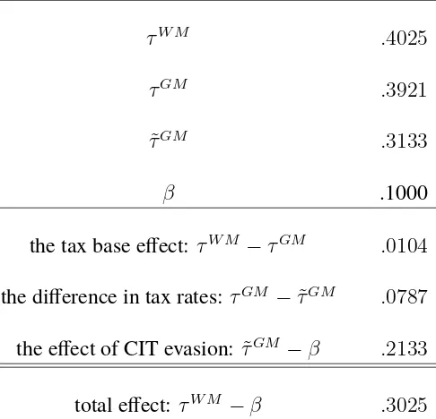
Table 2 provides the welfare-maximizing announced CIT rate,τW M, the growth-maximizing
announced rate, τGM, and the growth-maximizing effective CIT rate, τ˜GM for the benchmark
case. We find thatτW M =0.4025,τGM =0.3921, andτ˜GM =0.3133. The value of the optimal
CIT rate, 0.4025, is close to the estimated value of 42% by Aghion et al. (2016). As Propositions
3 and 4 indicate,τW M,τGM, andτ˜GM are all larger thanβ(= 0.1). Importantly, the difference
betweenτW M andβis 0.3025, which is quite large.
The fourth, fifth, and sixth rows of Table 2 provide a decomposition of the total effect,τW M−
β. The effect of CIT evasion,τ˜GM−β, amounts to 0.2133 and is largest of the three effects. Thus,
the effect of CIT evasion is the primary source of the high optimal CIT rate quantitatively.
Robustness
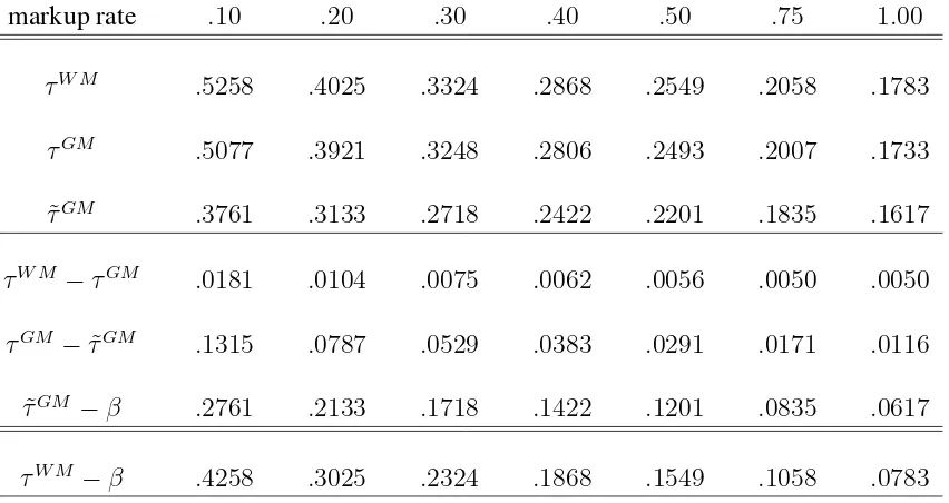
The effect of CIT evasion depends on the markup rateµ(= Γ(τ)/α−1) because it is related to their market power. Therefore, we calculate the optimal CIT rates for the various markup rates: see Table 3. 28
Insert Table 3 here.
Around the benchmark value (e.g., the case of markup rate= 0.1, ...,0.5), we find that both
τGM and τW M are much higher thanβ. In particular, the effect of CIT evasion, τ˜GM −β, is
significantly large for the alternative markup rates. This indicates that the effect of CIT evasion is the main source of the high optimal CIT rates.
Insert Table 4 here.
Unsurprisingly, the level of the optimal CIT rate substantially changes according to the output
elasticity of public services. However, we find that the impact of tax evasion remains relatively
28We choose the values ofαso that the markup rates take the values listed in Table 3. See also Appendix I for
strong for the alternative values ofβ, the output elasticity of public services. 29 In Table 4, we provide the ratio of the welfare-maximizing CIT rate to the output elasticity of public services,
τW M/β. Remember that the criterion in the comparison with the Barro rule is β. Thus, for example, althoughτW M ≈0.1in the case ofβ= 0.025, we can interpret this rate as a relatively
large value. Because the ratios in Table 4 show that the optimal CIT rates are much higher than
β, we can confirm the effect of tax evasion on the optimal CIT rate.
Next, we calculate the share of the effect of CIT evasion in the total effect, τ˜τW MGM−−ββ, for the
alternative values ofβ. In the benchmark case, the share is70%. For any case, the effect of CIT evasion occupies more than half of the total effect. This ensures the robustness of the relative importance of the effect of CIT evasion.
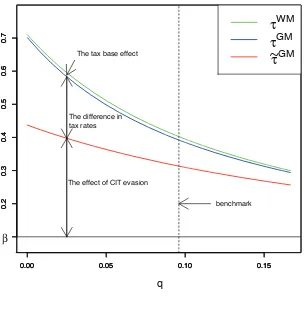
Finally, we conduct a robustness check of the main result with respect to audit rateq.
Insert Figure 1 here.
Figure 1 illustrates the result. Indeed, the level of the optimal CIT rate changes according to q. However, for the various alternative values ofq, we can confirm that the effect of CIT evasion is the dominant factor of the high optimal CIT rate relative to the output elasticity of public services.
30
6
Conclusion
This study investigates the optimal CIT in an endogenous growth model with productive public services, incorporating tax evasion by monopolistically competitive firms of intermediate goods.
We show that the growth- and welfare-maximizing CIT rates are higher than the output elas-ticity of productive public services. Thus, in view of tax evasion by firms, CIT should be higher
than the output elasticity of public services. This is mainly because the effect of CIT evasion mitigates the negative effect of CIT on growth and increases the benefit of raising the CIT rate
for the provision of productive public services.
29As we mentioned in the calibration section, the estimations ofβ lie in the neighborhood of0.10in existing
empirical studies. Although the quantitative performance of the model heavily depends onβ, the range considered here is sufficiently wide to keep the model quantitatively plausible.
30In particular, considerq= 0.089. This is the value chosen in Fullerton and Karayannis (1994). Table 5 shows
Under the plausible parameter values, our numerical exercises show that the effect of CIT evasion is significantly large and the optimal level of the CIT rate is much higher than the output
References
[1] Abiad, A., Furceri, D., and Topalova, P. (2016) The macroeconomic effect of public invest-ment: evidence from advanced econmics.Journal of Macroeconomics50, 224–240.
[2] Ag´enor, P.R. (2008) Health and infrastructure in a model of endogenous growth. Journal
of Macroeconomics30, 1407–1422.
[3] Ag´enor, P.R., and Neanisdis K. C. (2015) Innovation, public capital, and growth. Journal
of Macroeconomics44, 252–275.
[4] Aghion, P., U. Akcigit., J. Cag´e, and W. R. Kerr (2016) Taxation, corruption, and growth.
European Economic Review86, 24–51.
[5] Aghion, P., and P. Howitt (1998)Endogenous Growth Theory, MIT University Press,
Cam-bridge, MA.
[6] Allingham, M., and A. Sandmo (1972) Income tax evasion: a theoretical analysis.Journal
of Public Economics1, 323–338.
[7] Axtell, R. L. (2001) Zipf Distribution of U.S. Firm Sizes.Science293, 1818–1820.
[8] Barro, R. J. (1990) Government spending in a simple model of endogenous growth.Journal
of Political Economy98, 103–125.
[9] Barro, R. J. and X. Sala-i-Martin (2004) Economic Growth, 2nd edition. Cambridge, MA: MIT Press.
[10] Benassy, J. P. (1998) Is there always too little research in endogenous growth with expanding product variety? European Economic Review42, 61–69.
[11] Bom, P.R.D., and J.E. Ligthart (2014) What have we learned from three decades of research on the productivity of public capital? Journal of Economic Surveys28, 889–916.
[13] Chang S.-H., and Chang J.-J. (2015) Optimal government spending in and economy with imperfectly competitive goods and labor markets.Southern Economic Journal82, 385–407.
[14] Chatterjee, S., and S.J, Turnovsky. (2012) Infrastructure and inequality.European Economic
Review56, 1730–1745.
[15] Chen, B. L. (2003) Tax evasion in a model of endogenous growth. Review of Economic
Dynamics6, 381–403.
[16] Esfahani, H.S., and Ram´ırez, M.T. (2003) Institutions, infrastructure, and economic growth.
Journal of Development Economics70, 443–477.
[17] Fullerton, D. and M. Karayannis (1994) Tax evasion and the allocation of capital.Journal
of Public Economics95, 25–607.
[18] Futagami, K., Y. Morita, and A. Shibata (1993) Dynamic analysis of an endogenous growth
model with public capital.Scandinavian Journal of Economics95, 607–625.
[19] Ghosh, S., and U. Roy (2004) Fiscal policy, long-run growth, and welfare in a stock-flow
model of public goods.Canadian Journal of Economics37, 742–756.
[20] Glomm, G., and B. Ravikumar. (1994) Public investment in infrastructure in a simple
growth model.Journal of Economic Dynamics and Control18,1173–1187.
[21] Internal Revenue Service (2016) Federal Tax Compliance Research: Tax Gap Estimates for
Tax Years 2008-2010. Downloadable at https://www.irs.gov/pub/irs-soi/p1415.pdf.
[22] Internal Revenue Service (2017) IRS Data Book 2017, downloadable at
https://www.irs.gov/pub/irs-soi/17databk.pdf.
[23] Kafkalas, S., P. Kalaitzidakis, and V. Tzouvelekas (2014) Tax evasion and public
expendi-tures on tax revenue services in an endogenous growth model.European Economic Review
70, 438–453.
[25] Kamps, C. (2006) New estimates of government net capital stocks for 22 OECD countries, 1960–2001. IMF Staff Papers, 53, 120–150.
[26] Johannesen, N. (2010) Imperfect tax competition for profits, asymmetric equilibrium and beneficial tax havens.Journal of International Economics81, 253–264.
[27] Jones, L.E., Manuelli, R. and P. Rossi (1993) Optimal taxation in models of endogenous growth.Journal of Political Economy98, 1008–1038.
[28] National Tax Agency (2016) The 141th National Tax
Agency Annual Statistics Report FY 2015. Downloadable at http://www.nta.go.jp/publication/statistics/kokuzeicho/h27/h27.pdf.
[29] National Tax Agency (2017) National Tax Agency Report 2017. Downloadable at https://www.nta.go.jp/english/Report pdf/2017e.pdf.
[30] Peretto, P. F. (2007a) Corporate taxes, growth and welfare in a Schumpeterian economy.
Journal of Economic Theory137, 353–382.
[31] Peretto, P. F. (2007b) Schumpeterian growth with productive public spending and distor-tionary taxation.Review of Development Economics11, 699–722.
[32] Romer, P. (1986) Increasing returns and long-run growth.Journal of Political Economy94, 1002–1037.
[33] R¨oller, L.-H., and Waverman, L. (2001) Telecommunications infrastructure and economic development: A simultaneous approach.American Economic Review91, 909–923.
[34] Rotemberg, J. and Woodford, M. (1999) Oligopolistic Pricing and the Effects of Aggregate Demand.Journal of Political Economy100, 1153–1207.
[35] Roubini, N. and Sala-i-Martin, X. (1995) A growth model of inflation, tax evasion, and financial repression.Journal of Monetary Economics35, 275–301.
[36] Shioji, E. (2000) Public capital and economic growth: A convergence approach.Journal of
[37] Turnovsky, S.J. (1997) Fiscal policy in a growing economy with public capital.
Macroeco-nomic Dynamics1, 615–639.
Appendix
A
Proof of Lemma 1
Suppose that a firm declares its profit truthfully (π˜i,t = πi,t). Then, (7) can be rewritten as
πe
i,t = (1−τ)πi,t. This is maximized atpi,t =wt/(αb). From (6), we know that the firm’s true
profit is given by πi,t = (1−α)pi,tx(pi,t). Thus, if a firm setting the price at p˜i,t declares its
operating profit truthfully, (8) holds for the firm.
B
Proof of Proposition 1
Proof of (i): Sinceπ˜i,t ≤πi,t, (7) shows thatπi,te = {1−q(1 +s)τ}πi,t− {1−q(1 +s)}τπ˜i,t.
Thus, if1−q(1 +s)<0,πe
i,t increases with˜πi,t. Therefore, firms declare the largestπ˜i,t, which
is equal toπi,t because ofπ˜i,t ≤πi,t.
Since all firms declare their true profit, we have πe
i,t = (1 −τ)πi,t. The maximization of
πe
i,t = (1−τ)πi,t yieldsp˜i,t = wt/(αbi). We can obtain the true profit by substitutingp˜i,t into
(6). The expected after-tax profit follows from πe
i,t = (1−τ)πi,t. Sinceπ˜i,t = πi,t holds in (9),
we have˜τ =τ.
Next, if1−q(1 +s) = 0, we obtainπe
i,t = (1−τ)πi,t. In this case, the expected
after-tax profit is indifferent between whether a firm declares its profit truthfully. The maximization of πe
i,t = (1− τ)πi,t yields the same results as in the case of truth-telling firms, π˜i,t = πi,t,
˜
pi,t =wt/(αbi), andτ˜=τ.
Proof of (ii): We first prove the following lemma.
Lemma 2: Suppose1−q(1 +s)> 0. If a firm sets the price atp˜i,t, then the declared profit of the firm satisfies(8).
Proof of Lemma 2: To prove this lemma, we consider (a) firms that declare their operating profits truthfully and (b) firms that declare their operating profits dishonestly.
(a) Consider firms that declare their operating profits truthfully. Lemma 1 shows that the declared profit of these firms satisfies (8).
(b) We next consider the following two types of dishonest firms: those that do not declare (8) and those that declare (8).
Assumption (i), this firm is audited with probability one, q¯ = 1. Thus, the expected after-tax profit of this firm is given by
˜˜
πi,te =πi,t−τπ˜˜i,t −1×(1 +s)τ (
πi,t−π˜˜i,t )
. (B.1)
We next consider a dishonest firm that declares (8). From Assumption (ii), this firm is audited with a probability lower than one, q¯= q ∈ [0,1). The expected after-tax profit of this type of dishonest firms is given by
˜
πi,te =πi,t−τπ˜i,t−q(1 +s)τ(πi,t−π˜i,t). (B.2)
Supposeπ˜e
i,t <π˜˜ei,tholds. This implies that a dishonest firm declaresπ˜˜i,t, which is not equal
to (8). Using (B.1) and (B.2), we rearrangeπ˜e
i,t <π˜˜i,te as follows:
πi,t−τπ˜i,t−q(1 +s)τ(πi,t−π˜i,t)< πi,t−τ˜˜πi,t−(1 +s)τ (
πi,t−π˜˜i,t )
,
⇔ (1 +s)(1−q)πi,t−[1−q(1 +s)]˜πi,t < sπ˜˜i,t,
⇒ (1 +s)(1−q)πi,t−[1−q(1 +s)]˜πi,t < sπi,t,
⇔ [1−q(1 +s)]πi,t <[1−q(1 +s)]˜πi,t.
The third line uses the factπ˜˜i,t ≤πi,t. If1−q(1 +s)>0, the inequality in the last line indicates
π < π˜i,t, which contradictsπ˜˜i,t ≤πi,t. Thus, dishonest firms declare (8). Lemma 2 is proved.
From Lemma 2, we have thatπe
i,t = (1−τ˜)πi,t = [1−q(1 +s)τ]πi,t−[1−q(1 +s)]τπ˜i,t,
whereπ˜i,tis given by (8). Firms maximize thisπi,te by choosingpi,t. The first-order condition is
given by
∂πe i,t
∂p˜i,t
=LY,t(αA) 1 1−αG
α
1−α t p˜
− 1
1−α i,t
×
{
1−q(1 +s)τ
(1−α)bi (
−αbi+
wt
˜
pi,t )
+ [1−q(1 +s)]τ α
}
= 0 (B.3)
Since1−q(1 +s) > 0holds, we have that0 <(1−α)[1−q(1 +s)]τ < [1−q(1 +s)]τ <
hence, p˜i,t > wt/(αbt). If we substitute (11) into (6), we obtain (12). Fromπi,te = (1−τ˜)πi,t
and (12), we obtain (13).
Here, let us define
γ(τ)≡Γ(τ)−1
= 1−(1−α)[1−q(1 +s)]τ
1−q(1 +s)τ (<1). (B.4)
Substituting (8) and (12) into (9), we have
˜
τ
τ = [1−q(1 +s)]
1−α
1−αγ(τ)+q(1 +s) (B.5)
First, we can easily show that τ < τ˜ because of[1−q(1 +s)] 1−α
1−αγ(τ) +q(1 +s)−1 = [1−
q(1 +s)][ 1−α
1−αγ(τ) −1
]
<0, whereγ(τ)<1and1−q(1 +s)>0.
Second, from the definition ofγ(τ)and (B.5), lim
τ→0τ˜ = 0
and ˜τ|τ=1 =
1 +αq(1 +s) 1 +α , and
therefore, we haveτ˜∈(0,1+αq1+(1+α s)].
C
Relationship between
τ
˜
and
τ
From (B.4), we obtain
γ′
(τ) =−(1−α)[1−q(1 +s)]
[1−q(1 +s)τ]2 <0, (C.1)
dγ(τ)
dq =
(1−α)(1−τ)τ(1 +s)
[1−q(1 +s)τ]2 >0, (C.2)
or bothΓ′
(τ) > 0anddΓ(τ)/dq < 0. From (B.5) and (C.1), we obtaind(τ /τ˜)/dτ > 0. From (B.5), (C.2), andγ(τ)<1, we obtaind(τ /τ˜)/d(q(1 +s))<0.
Finally, we provedτ /dτ >˜ 0. From (B.5),
dτ˜
dτ =
[1−q(1 +s)](1−α)
[1−αγ(τ)]2 [1−αγ(τ) +ατ γ
′
(τ)] +q(1 +s) (C.3)
Thus, we have ddτ˜τ >0, if and only if
1−αγ(τ) +ατ γ′
(τ)>−[1−αγ(τ)]
2q(1 +s)
[1−q(1 +s)](1−α) (C.4)
Fromγ′
(τ)<0andγ′′
(τ)<0, dτd[1−αγ(τ) +ατ γ′
(τ)] =−αγ′
(τ) +ατ γ′′
indicates that the LHS of (C.4) is decreasing inτ. Furthermore, the RHS of (C.4) is decreasing in τ because of γ(τ) < 1 and γ′
(τ) < 0. Thus, dτd˜τ > 0 for anyτ ∈ (0,1)if the minimum value of the LHS of (C.4),1−αγ(1) +ατ γ′
(1), is larger than the maximum value of the RHS,
−[1−αγ(0)]2q(1+s)
[1−q(1+s)](1−α). Usingγ(0) = 1,γ(1) =αandγ ′
(1) = − 1−α
1−q(1+s), we obtain
1−αγ(1) +ατ γ′
(1)−
{
−[1−αγ(0)]
2q(1 +s)
[1−q(1 +s)](1−α)
}
= (1−α)[1−αq(1 +s)]
1−q(1 +s) >0, (C.5)
and therefore, ddττ˜ >0for anyτ ∈(0,1).
D
Derivation of equilibrium conditions
The price level of firmiandj whose productivity isbi andbj isp˜i,t = αbΘiwtandp˜j,t = αbΘjwt,
whereΘ = 1(Γ(˜τ))for1−q(1+s)≤(>)0. Combining these with (3) yields pi,t
pj,t = (
xi,t
xj,t
)α−1
=
bj
bi. Thus, we havexi,t =
(b
j
bi
) 1
α−1
xj,t. This together with (1), (2), and (3) rewritesp˜i,t = αbΘiwt
into
xi,t =
α2L Y,t
(1−α)Θb
1
α−1 i
∫
b1−ααdF(b)Nt
. (D.1)
From (19) and (D.1), we obtain labor employed in the final good sector as follows:
LY,t =
(1−α)Θ
(1−α)Θ +α2L. (D.2)
Substituting (D.2) into (D.1) leads to
x(˜pi,t) = [
α2
(1−α)Θ +α2 ]
b
1 1−α i ∫
b1−ααdF(b)
L Nt
. (D.3)
From (1) and (3), we obtain ∫0Ntpi,txi,tdi = αYt. Combining
∫Nt
0 pi,txi,tdi = αYt with
πe
i,t = (1 − τ˜) (1−αΘ
−1
) ˜pi,tx(˜pi,t), we obtain the total expected after-tax operating profit,
Nt ∫
πe
i,tdF(b) = (1−τ˜)(1−αΘ
−1
)αYt. By combining the total expected after-tax operating
profit with (5), we obtain the gross interest rate
Rt−1 =
(1−τ˜)(1−αΘ−1
)αYt
ηNt
Combining πi,t = (1 − αΘ−1)˜pi,tx(˜pi,t) with
∫Nt
0 pi,txi,tdi = αYt, the budget constraint
of the government (17) is rewritten into Gt +Mt = ˜τ(1− αΘ−1)αYt. Dividing both sides
of the final good market clearing condition, Yt = Ct + ηNt+1 +Gt +Mt, by Nt and using
Gt+Mt = ˜τ(1−αΘ−1)αYtyield
Nt+1
Nt
= 1
η
{ [
1−˜τ(1−αΘ−1)
α] Yt Nt −
Ct
Nt }
, (D.5)
and substituting (D.4) into (15), we obtain
Ct+1
Ct
=
[
(1−˜τ) (1−αΘ−1
)α
(1 +ρ)η
Yt+1
Nt+1
]1/σ
. (D.6)
Substitutingπi,t = (1−αΘ−1) ˜pi,tx(˜pi,t)into (18) reduces toGt = [1−Q(q)]˜τ(1−αΘ−1)αYt.
Combining it with (1), (D.2), and (D.3), we obtain Yt
Nt = Ω(˜τ). Substituting
Yt
Nt = Ω(˜τ) into
(D.5) and (D.6) and dividing (D.6) by (D.5) leads to (20).
E
Proof of Proposition 2
Let us define the right-hand side (RHS) of (20) as ϑ(zt) ≡ η
1−σ1[(1−τ˜)(1−αΘ−1)αΩ(˜τ)/(1+ρ)]1/σzt [1−τ˜(1−αΘ−1)α]Ω(˜τ)−zt .
Here, note that the denominator ofϑ(zt): [1−τ˜(1−αΘ−1)α]Ω(˜τ)−zt must be positive, that
is, zt < z¯ ≡ [1−τ˜(1− αΘ−1)α]Ω(˜τ), otherwise Nt eventually equals to zero from (D.5): Nt+1
Nt = 1
η {[1−τ˜(1−αΘ
−1
)α] Ω(˜τ)−zt}. WhenNt = 0, both output and consumption equal
to zero, which violates the first order condition of the representative household.
The properties ofϑ(zt)forzt∈[0,z¯)are as follows:
ϑ(0) = 0, lim
zt→z¯ϑ(zt) = +∞,
ϑ′
(zt) =
η1−1
σ[(1−τ˜)(1−αΘ−1)αΩ(˜τ)/(1 +ρ)]1/σ[1−τ˜(1−αΘ−1)α]Ω(˜τ)
{[1−τ˜(1−αΘ−1)α]Ω(˜τ)
−zt}2
>0,
ϑ′
(0) = η[(1−τ˜) (1−αΘ
−1
)α(1 +ρ)−1
η−1
Ω(˜τ)]1/σ [1−τ˜(1−αΘ−1)α] Ω(˜τ) , zlim
t→z¯ϑ ′
(zt) = +∞
ϑ′′
(zt) =
2η1−1
σ[(1−τ˜)(1−αΘ−1)αΩ(˜τ)/(1 +ρ)]1/σ[1−τ˜(1−αΘ−1)α]Ω(˜τ)
{[1−τ˜(1−αΘ−1)α]Ω(˜τ)
−zt}3
>0. (E.1)
(E.1) indicates that ϑ(zt)is monotonically increasing and convex function of zt and takes zero
On the other hand, the left-hand side (LHS) of (20) represents45◦
line. Thus, we find that a unique steady statezˆ∈(0,z¯), which is unstable exists if and only ifϑ′
(0) <1holds. From (D.5), (D.6) andYt/Nt = Ω(τ),Ct,Nt, andYtgrow at the same constant rate,Ct+1/Ct=Nt+1/Nt=
Yt+1/Yt = ˆg in the steady state.
The rest of this appendix shows that the TVC (16) ensures ϑ′
(0) < 1. (23) and the asset market clearing condition, Wt = ηNt+1 together with the assumption N0 = 1 transform the
TVC (16) into limt→∞
ˆ
z−σˆgt(1−σ)
(1+ρ)t = 0. To satisfy the TVC, 1 > (1 + ρ)
−1
ˆ
g1−σ
must holds.
1>(1 +ρ)−1
ˆ
g1−σ
and (23) together with (11−−ττ˜˜(1)(1−−ααΘΘ−−11))αα <1lead toϑ
′
(0) <1.
F
Proof of Proposition 3
F.1 Proof of 1
In this case, since each firm does not evade CIT,Θ = 1and˜τ =τ. Then, by (21) and (23), we obtainτ˜GM =τGM =αimmediately.
F.2 Proof of 2
In the beginning, note that the decision of optimal announced CIT rate is equivalent to that of the optimal effective CIT rate. This is becauseτ˜is the function ofτ from (B.5), andτ˜is strictly increasing inτ,dτ /dτ >˜ 0, for anyτ ∈(0,1], as shown in Appendix C.
Because the growth rate converges to0asτ goes to0by the construction of the model, the growth rate is maximized at1or some interior point in(0,1).
First, we prove that the growth-maximizing effective CIT is higher thanαwhen it is an interior point in(0,1). From the definition ofΩ(˜τ)and (D.6), growth maximization with respect toτ˜is equivalent tomax
˜
τ f(˜τ) = ln(1−˜τ)˜τ
α
1−α[1−αγ(τ)] 1 1−αγ(τ)
[
γ(τ) 1−α+α2γ(τ)
] 1
1−α
, subject to (B.5):
˜ τ
τ = [1−q(1 +s)] 1−α
1−αγ(τ) +q(1 +s). The first derivative off(˜τ)is
f′
(˜τ) =
[
− 1 1−˜τ +
α
1−α
1 ˜
τ
| {z }
≡Ψ1(˜τ)
]
+ α 1−α
dτ dτ˜γ
′
(τ)
[
1
γ(τ)− 1
1−αγ(τ)−
α
1−α+α2γ(τ)
| {z }
≡Ψ2(τ)
]
.
(F.1) It is obvious thatΨ1(˜τ) = −1−1τ˜ +
α 1−α
1 τ =
α−τ˜
sign ofΨ2(τ)is negative forτ˜≤α.
signΨ2(τ) = [1−αγ(τ)][1−α+α2γ(τ)]−γ(τ)[1−α+α2γ(τ)]−αγ(τ)[1−αγ(τ)]
=−α3γ(τ)2−(1−α)[(1 + 2α)γ(τ)−1] (F.2)
Here, signΨ2(τ) < 0 for γ(τ) > 1+21α. Furthermore, (B.4) and (B.5) indicate that γ(τ) is
increasing inq(1+s)and whenq(1+s) = 0,γ(τ) = 1−(1−α)τ,τ = 1−τ˜ατ˜andγ(
˜ τ 1−α˜τ) =
1−τ˜
1−ατ˜
hold. From 1−τ˜
1−ατ˜ −
1 1+2α =
α−τ˜+α(1−τ˜)
(1−ατ˜)(1+2α) > 0, we obtainγ(
˜ τ 1−ατ˜) =
1−˜τ
1−ατ˜ >
1
1+2α for ˜τ ≤ α.
Thus, signΨ2(τ)<0forτ˜≤α. CombiningΨ1(˜τ)≥0andΨ2(˜τ)<0forτ˜≤αwithγ′(τ)<0
((B.5)) and ddττ˜ > 0, we obtain f′
(˜τ) > 0for τ˜ ≤ α. From the discussion so far, we find that
˜
τGM > αholds.
Next, we consider the case of the corner solution of growth-maximization: τGM = 1.
As-sumingq(1 +s)> α(1+α)−1
α additionally, we ensure that˜τGM > αbecauseτ˜|τ=1 =
1+αq(1+s) 1+α .31
G
Proof and intuition of Proposition 4
(i) Proof of 1
The maximization condition of social welfare is ∂U∂τ = 0. By (26), this is equivalent to
[
1−(1 +ρ)−1
ˆ
g1−σ]∂zˆ
∂τ + (1 +ρ)