Munich Personal RePEc Archive
Deaths in the Family
Borooah, Vani
University of Ulster
May 2018
Chapter 2: Deaths in the Family
Abstract
The purpose of this chapter is to evaluate the relative strengths of economic and social status in determining deaths in households in India. The first part of the chapter focuses on the “age at
death” using National Sample Survey data for 2004 and 2014. The purpose was to ask if, after controlling for non-community factors, the fact that Indians belonged to different social groups,
encapsulating different degrees of social status, exercised a significant influence on their age at death? The existence of a social group effect would suggest that there was a “social gradient” to health
outcomes in India. The second part of the chapter, using data from the Indian Human Development Survey of 2011, investigated the determinants of infant and child mortality. The overriding concern now is gender bias with girls more likely to die than boys before attaining their first (infant) and fifth
(child) birthdays. As this study has shown, gender bias in infant and child mortality rates is, with singular exceptions, a feature of all the social groups. In conducting this investigation, the chapter
addresses for India an issue which lies at the heart of social epidemiology: estimating the relative strengths of individual and social factors in determining mortality outcomes.
JEL: D53 I12, O15
1 2.1. Introduction
The publication of the Black report (Black et. al., 1980) spawned a number of studies in
industrialised countries which examined the social factors underlying health outcomes. The
fundamental finding from these studies, particularly with respect to mortality and life expectancy, was
the existence of “a social gradient” in mortality: “wherever you stand on the social ladder, your
chances of an earlier death are higher than it is for your betters” (Epstein, 1998). The social gradient
in mortality was observed for most of the major causes of death: for example, Marmot (2000) showed
that, for every one of twelve diseases, the ratio of deaths (from the disease) to numbers in a Civil
Service grade rose steadily as one moved down the hierarchy.
Since, in the end, it is the individual who falls ill, it is tempting for epidemiologists to focus
on the risks inherent in individual behaviour: for example, smoking, diet, and exercise. However, the
most important implication of a social gradient to health outcomes is that people’s susceptibility to
disease depends on more than just their individual behaviour; crucially, it depends on the social
environment within which they lead their life (Marmot, 2000 and 2004). Consequently, the focus on
inter-personal differences in risk might be usefully complemented by examining differences in risk
between different social environments.
For example, even after controlling for inter-personal differences, mortality risks might differ
by occupational class. This might be due to the fact that while low status jobs make fewer mental
demands, they cause more psychological distress than high status jobs (Karasek and Marmot, 1996;
Griffin et. al., 2002; Marmot, 2004) with the result that people in higher level jobs report significantly
less job-related depression than people in lower-level jobs (Birdi et.al., 1995).
In turn, anxiety and stress are related to disease: the stress hormones that anxiety releases
affect the cardiovascular and immune systems with the result that prolonged exposure to stress is
likely to inflict multiple costs on health in the form of inter alia increased susceptibility to diabetes,
2
and Marmot, 1999). So, the social gradient in mortality may have a psychosocial basis, relating to the
degree of control that individuals have over their lives.1
The “social gradient to health” is essentially a Western construct and there has been very little
investigation into whether, in developing countries as well, people’s state of health is dependent on
their social status. For example, in India, which is the country studied in this chapter, we know from
studies of specific geographical areas that health outcomes differ systematically by gender and
economic class (Sen, Iyer, and George, 2007). In addition, local government spending on public
goods, including health-related goods, is, after controlling for a variety of factors, lower in areas with
greater caste fragmentation compared to ethnically more homogenous areas (Sengupta and Sarkar,
2007).
Considering India in its entirety, two of its most socially depressed groups - Adivasis2 and the
Scheduled Castes (Dalits)3
- have some of the worst health outcomes: for example, as Guha (2007)
observes, 28.9 percent of Adivasis and 15.6 percent of Dalits have no access to doctors or clinics and
only 42.2 percent of Adivasi children and 57.6 percent of Dalit children have been immunised. Of
course, it is possible that the relative poor health outcomes of India’s socially backward groups has
less to do with their low social status and much more to do with their weak economic position and
with their poor living conditions. The purpose of this chapter is to evaluate the relative strengths of
economic and social status in determining the health outcomes of persons in India. In other words,
even after controlling for non-community factors, did the fact that Indians belonged to different social
groups, embodying different degrees of social status, exercise a significant influence on the state of
their health?
The first health outcome is that of “age at death” and the question here is whether, after
controlling for non-social factors, there was a significant difference between persons from different
1 Psychologists distinguish between stress caused by a high demand on one’s capacities – for example, tight
deadlines – and stress engendered by a low sense of control over one’s life.
2 There are about 85 million Indians classified as belonging to the “Scheduled Tribes”; of these, Adivasis
(meaning original inhabitants”) refer to the 70 million who live in the heart of India, in a relatively contiguous hill and forest belt extending across the states of Gujarat, Rajasthan, Maharashtra, Madhya Pradesh,
Chhattisgargh, Jharkhand, Andhra Pradesh, Orissa, Bihar, and West Bengal (Guha, 2007).
3 The Scheduled Castes (or, Dalits), who number about 18 million, refer to those who belong to the formerly
3
social groups in the age at which they died. The second health outcome concerns deaths of infants and
young children. The relevant question here is the relative strength of factors that determined the rates
of infant and of child mortality – defined as the proportion of live births that did not survive their first
(infant mortality) and fifth years (child mortality). Anticipating the results presented in subsequent
sections of this chapter, the central conclusion with respect to infant and child deaths is that the social
gradient is supplemented by a “gender bias” in infant survivals – with males more likely to survive
their first and fifth years than females – allied to a “geographic gradient” by which the size of the
gender bias in infant and child survivals depended on where in India the births occurred. This gender
bias affects all the social groups, and two of the five regions, distinguished in this chapter.
In broad terms, the adverse female to male ratio in South Asian countries stems from the
unequal treatment of women.4 This could take the form of “natal inequality” where the preference for
sons, in conjunction with modern techniques to determine the gender of the foetus, results in
sex-selective abortions. This type of inequality is particularly prevalent in countries of East and South
Asia (Sen, 2001). It could also take the form of “mortality inequality” whereby there is, relative to
boys and men, a general neglect of girls and women in respect of factors that contribute to physical
well-being: for example, girls and women could be relatively deprived in terms of their diet and in
terms of their access to, and utilisation of, health care facilities (Borooah, 2004). Natal inequality and
mortality inequality then combine to ensure that there are fewer women than men in countries where
such forms of gender discrimination are particularly marked. Bongaarts and Guilmoto (2015)
conclude, however, that, in spite of the recent rise in prenatal selection, excess mortality has been, and
is expected to remain, the dominant cause of missing females.
2.2 Health Data from the National Sample Survey for India
The age at death of persons was analysed using data from the 60th Round (January-June 2004)
and the 71st Round (January-June 2014) of the specialist Morbidity and Health Care Surveys of the
National Sample Survey (NSS).5 Hereafter, these are referred to in the chapter as, respectively, the
4 The female to male ratio is substantially below unity in several developing countries: in 2015, it was 0.94 in
4
71st NSS and the 60th NSS. 6 The 60th NSS surveyed 73,911 (grossed up, 1,982,395) households and
the 71st Round surveyed 65,975 (grossed up, 2,479,214) households. An item of particular interest to
this study was the construction of the social groups with each person in the estimation sample being
placed in one, and only one, of these groups. The NSS categorised persons by four social groups
(Scheduled Tribes (ST); Scheduled Castes (SC); Other Backward Classes (OBC); and ‘Others’ and
simultaneously by eight religion groups (Hindus; Islam; Christianity; Sikhism; Jainism; Buddhism;
Zoroastrianism; ‘Other’). Combining the NSS ‘social group’ and ‘religion’ categories, we subdivided
households into the following groups which are used as the basis for analysis in this chapter:
1. Scheduled Tribes (ST). These comprised 9.1 percent of the grossed up 2,479,214 households
in the 71st NSS round and 8.3 percent of the grossed up 1,982,395 households in the 60th NSS:
approximately 85.5 percent of these households were Hindu and 9.3% were Christian.7
2. Scheduled Castes (SC). These comprised 18.6 percent of the grossed up 2,479,214
households in the 71st NSS and 20.1 of the grossed up 1,982,395 households in the 60th NSS
and 94% of the households in this category in the 71st NSS were Hindu.8
3. Non-Muslim Other Backward Classes (NMOBC). These comprised 36.8 percent of the
grossed up 2,479,214 households in the 71st NSS and 35.7 percent of the grossed up
1,982,395 households in the 60th NSS and 97 percent of the households in this category in the
71st NSS were Hindu.
4. Muslims. These comprised 12.5 percent of the grossed up 2,479,214 households in the 71st
NSS and 10.8 percent of the grossed up 1,982,395 households in the 60th NSS.9
5. Non-Muslim upper classes (NMUC). These comprised 23 percent of the grossed up 2,479,214
households in the 71st NSS round and 25.1 percent of the grossed up 1,982,395 households in
the 60th NSS; 93.4 percent of the households in this category in the 71st NSS were Hindu.
6 It is important to draw attention to the fact that all the results reported in it are based upon grossing up the
survey data using the observation-specific weights provided by the NSS for each of the surveys.
7 Figures relate to the 71st Round. The 60th Round figures are similar and not shown. This category also included
3,063 Muslim households. Since Muslim ST persons are entitled to reservation benefits these households have been retained in the ST category.
8 This category also included some Muslim households. Since Muslims from the SC are not entitled to SC
5
In addition to information about the social group of the households, the Surveys also provided
information about the households’ living conditions. Listed below is information about these
conditions that was reported in both the 60th and the 71st Rounds and the variables constructed for the
purposes of this study from this information:
1. The first component of living conditions related to the quality of the latrines used by the
deceased: the variable “latrine” was assigned the value 1 if the latrines were flushing toilets or
emptied into a sceptic tank; and 0 otherwise.
2. The second component of living conditions related to the quality of the drains: the variable
“drain” was assigned the value 1 if the drains associated with the deceased’s home were
underground or were covered pucca; and 0 otherwise.
3. The third component of living conditions related to the quality of the source of drinking
water used by the deceased: the variable “water source” was assigned the value 1 if the source
of drinking water was from a tap; and 0 otherwise.
4. The fourth component of living conditions related to the nature of the cooking fuel used by
the deceased’s household: the variable “cooking fuel” was assigned the value 1 if the cooking
fuel was gas, gobar gas, kerosene, or electricity; and 0 otherwise.
2.3 The Age at Death in Households
Each household was asked if there had been a death (or deaths) in the household in the
previous 365 days and particulars of these deaths: 2,395 households (grossed up to 34,857households)
and 1,716 households (grossed up to 35,766) households reported that there been such deaths for,
respectively the 71st and 60th NSS. 10 The specific information that this study was interested in was
the age at death of the person concerned and specifically, whether the age at death varied with respect
to the five social groups distinguished in this study: Scheduled Tribe (ST), Scheduled Caste (SC),
Non-Muslim Other Backward Classes (NMOBC), Muslims, and Non-Muslim Upper Class (NMUC).
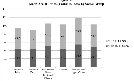
<Figure 1>
10 Of the 1,716 households in the 60th Round, reporting deaths in the previous year: 1,634 households reported a
6
Figure 1 shows that, in the 71st NSS (2014), the mean age at death was highest for persons
from NMUC households (63.2 years) and lowest for persons from ST households (46 years).11 In the
10 years between the 60th and 71st Round, the mean age at death had increased for all households
reporting a death: from: 43.3 to 46 years for SC households; 49.7 to 55.3 years for NMOBC
households; 43.6 to 59.4 years for Muslim households; and 54.5 to 63.2 years for NMUC households.
Overall, the mean age at death increased by nearly seven years in the 10 year period 2004 to 2014,
from 48.3 in the 60th round to 54.8 years in the 71st round.
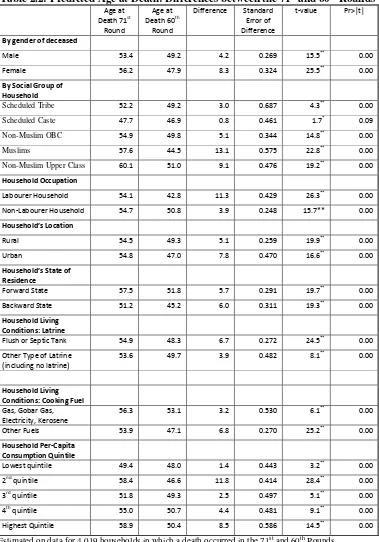
<Table 2.1>
Table 2.1 shows the results from a regression of the age at death of persons from households
in which a death (or deaths) occurred in the 71st Round (2,384 sample households, grossed up to
34,853 households ) and the 60th Round (1,708 households, grossed up to 33,598 households) using
the following explanatory variables:
1. The gender of the deceased
2. The social group of household (defined earlier) in which the death occurred
3. Whether the household, in which the death occurred, was a ‘casual labourer’ household or,
else, was self-employed or in regular salaried employment.
4. Whether the household, in which the death occurred, lived in a rural or urban area.
5. Whether the household, in which the death occurred, lived in a ‘forward’ or a ‘backward’
state.12
6. The quality of the household’s latrine and cooking fuel, as discussed above.
7. The quintile of monthly household per capita consumption expenditure (HPCE) to which the
household belonged from lowest (=1) to highest (=5).
11 All the figures in Figure 1 relate to households whose social group was defined in terms of one of the five
categories: ST, SC, NMOBC, Muslim, and NMUC. Of the 2,395 households which reported a death in the 71st round, and of the 1,716 households which reported a death in the 60th round, social group was defined for, respectively, 2,384 and 1,708 households.
12 For the 71st Round: Forward States were Himachal; Punjab; Chandigarh; Haryana; Delhi; West Bengal;
Gujarat; D&D; D&N Haveli; Maharashtra; AP; Karnataka; Goa; Kerala; TN; Pondicherry; Telangana;
Backward States were: Uttaranchal; Rajasthan, UP, Bihar; Sikkim; Arunachal; Nagaland; Manipur; Mizoram;
7
The results from the estimated equation are presented in Table 2.1 in the form of the predicted
age at death (PAD) from the estimated regression coefficients of the ‘age at death’ equation where
these predictions relate to the average age at death.13 It should be emphasised, in respect of the
predictions shown in Table 2.1, that the relationship between social group and the age at death was
analysed on a ceteris paribus basis that is after controlling for the effects of the variables 1-5, above.
Consequently, the PAD for the five social groups shown in Table 2.1 will, and do, differ from the
sample ages at death shown in Figure 2.14 It should also be emphasised that, in the estimation, each
observation in the sample was weighted by its corresponding weight as provided by the NSS.
The second column of Table 2.1 shows that, for the 71st Round, after controlling for other
variables, NMUC households had the highest PAD (60.5 years) followed by Muslim households (58
years), followed by NMOBC households (55.2 years), followed by ST households (52.6 years) with
SC households predicting the lowest ADD (48 years). These PAD for each social group (say, NMUC)
was computed by assuming that all the 2,383 households in the 71st (or, as the case may be, the 60th)
round were from that social group (NMUC), the values of the other attributes being as observed in the
sample. Applying the NMUC coefficient applied to the household attributes yielded the age of death
for deaths in each of the 2,383 households. The mean of these ages was the PAD for this social group
(NMUC) under this scenario: this was 60.5 years for the 71st round and 50.3 years for the 60th round.
The PAD for the other social groups were computed in similar fashion. Since the only factor that was
different between these five ‘social group’ scenarios was the households’ social group (ST, SC,
NMOBC, Muslims, and NMUC), the observed differences between these five PAD were entirely the
result of differences in the households’ social group.
The marginal PAD, shown in column 3 of Table 2.1, are the differences between the PAD of
the ST, SC. NMOBC, and Muslim households and that of (the reference) NMUC households. Column
4 shows the standard error associated with these marginal probabilities and the t values – obtained by
dividing the marginal probability (shown in column 3) by its standard error (shown in column 5) – are
13 Following the advice of Long and Freese (2014).
14 For example, if living in a ‘forward’ state raises the average age at death and if ST households are
8
shown in column 5. Lastly, column 6 shows, under the null hypothesis that the marginal probability
was zero, the probability of obtaining a t-value in excess of the (absolute value of) calculated value.
The fact that these were less than 5% shows that all the social group marginal PAD, for both the 71st
and the 60th NSS, were significantly different from zero. In other words, the PAD for households
from the four social groups (ST, SC, NMOBC, and Muslims) were all significantly lower than for
NMUC households in 2014 and in 2004.
For both the 71st and the 60th NSS and, the difference in the PAD was significantly different
for Muslim households compared to NMOBC households (58 versus 55.2 years for the 71st round and
43.8 versus 49.1 years for the 60th round) and between households from the Scheduled Tribes and the
Scheduled Castes (52.6 versus 48 years for the 71st round and 48.5 versus 46.1 years for the 60th
round. The PAD of female deaths was significantly higher than that of male deaths in the 71st round
(56.4 versus 53.6 years) but significantly lower (47.3 versus 48.6 years) in the 60th round.
The non-social group variables showed that, compared to being a labourer, a non-labouring
job significantly increased the PAD: by 0.6 years in the 71st NSS and by 8.0 years in the 60th NSS. 15
Similarly, compared to living in a ‘forward’ state, living in a ‘backward’ state significantly reduced
the PAD by 6.3 years in the 71st NSS and by 6.6 years in the 60th NSS. Compared to living in a rural
area, living in an urban area significantly reduced the PAD by 2.3 years in the 60th NSS but, in the 71st
NSS, there was no significant difference between the PAD in rural and urban locations. Lastly, in
terms of living condition, the most pernicious effect on the age at death in households was the type of
cooking fuel that it used: in both the 71st and the 60th Rounds, the age at death was significantly lower
in households that used fossil fuel for cooking instead of gas or electricity.
A noticeable feature of the PAD from the 71st and the 60th Rounds is that, in the 10 years
separating the two rounds, the predicted ages at death increased for all the groups
For the ST from 48.5 to 52.6 years
for the SC from 46.1 to 48 years;
for the NMOBC from 49.1 to 55.2 years;
9
for Muslims from 43.8 to 58 years
for the MUC from 44.3 to 48.5 years
for the NMUC from 50.3 to 60.5 years
However, from a policy perspective, the relevant issue is whether these improvements were
statistically significant or whether they could be accommodated within a ‘no change’ null hypothesis.
In order to answer this question we re-estimated the ‘age at death’ equation, specified in Table 2.1,
jointly over all the relevant observations for the 71st round and 60th Rounds (a total of 4,019
observations on households which reported a death) and then tested whether the PAD was
significantly different between the two rounds.
<Table 2.2>
Columns 2 and 3 of Table 2.2 show the PAD for, respectively, the 71st and the 60th NSS while
column 4 records the difference; column 5 shows the standard error the difference and column 6
shows the t-value associated with difference, computed by dividing the difference by its standard error
and column 7 shows the probability of obtaining a t value great than under the null hypothesis that the
difference was zero. These PAD for the 71st NSS, for NMUC households, were computed by
assuming that all the 4,019 households in the combined sample were NMUC from the 71st NSS (that
is, the 71st NSS coefficient for NMUC applied to their attributes) and computing the PAD under this
scenario: this was 60.1 years (column 2). Similarly, the PAD for the 60th NSS for the NMUC
households were computed by assuming that all the 4,019 households in the combined sample were
NMUC from the 60th NSS (that is, the 60th NSS coefficient for NMUC applied to their attributes) and
computing the PAD under this scenario: this was 51 years (column 3). The difference between the
two rounds in their PAD for NMUC households was 9.1 years (column 4) and, as the t-value in
column 6 shows, this was difference significantly different from zero.
Table 2.2 shows that the PAD was significantly higher in 2014 than in 2004 for households
from all the social groups, except the SC for which there was no significant difference between the
PAD from the two rounds. For labourer and non-labourer households the PAD was significantly
higher in the 71st, compared to the 60th, Round (54.1 versus 42.8 years for labourer households and
10
higher for rural households, and for urban households, in the 71st, compared to the 60th, Round (54.5
versus 49.3 years for rural households and 54.8 years versus 47 years for urban households). Lastly,
the PAD was significantly higher for households in forward states, and for households in backward
states, in the 71st, compared to the 60th, Round (57.5 versus 51.8 years for households in forward
states and 51.2 years versus 45.2 years for households in backward states).
2.4. Infant and Child Deaths
A number of empirical studies have examined demographic outcomes in India and in other
countries with respect to fertility and infant and child mortality rates (inter alia Caldwell, 1979 and
1986; Subbarao and Rainey, 1992; Murthi et. al., 1995; Borooah, 2000). However, a weakness of
these studies is that while they purported to examine the behaviour of individuals, they were, in fact,
based on data pertaining to geographical units. For example, Murthi et. al., (1995) and Borooah
(2000) were both based on district-level data. The dangers of inferring individual behaviour from an
analysis of aggregate data were recognised, nearly half a century ago, by Theil (1954): “when models
of individual behaviour are estimated from variation in average behaviour and average conditioning
variables for large aggregates …[then] the properties of the estimates depend upon many tenuous
aggregation assumptions”. But, given the paucity of large sets of data relating to individuals,
researchers sought exculpation in the fact that there was no alternative.
Parikh and Gupta (2001) enquired into the effectiveness of female literacy in reducing fertility
in the two Indian states of Andhra Pradesh and Uttar Pradesh, using unit record data for ‘ever
married’ women from the National Family Household Survey’s 1992-93 data set. In a similar vein,
Borooah (2003) examined the determinants of fertility and infant survivals using unit record data from
a survey of 33,000 rural households for 1993-94, commissioned by the Indian Planning Commission,
funded by a consortium of United Nations agencies, and carried out by the National Council of
Applied Economic Research.16 In so doing, both sets of authors noted that, to the best of their
knowledge, these data had not been used for the multiple regression analysis of the relationship
between literacy and fertility.
16 This Survey, described in Shariff (1999) was the precursor to the Survey data used in this chapter, discussed
11
These observations then point to a general problem that vitiates empirical studies of
demographic outcomes India: when they are cast in a multiple regression mould, their results are
derived from aggregate data; on the other hand, when they are based on unit record data they do little
more than present bi-variate cross-tabulations17. This chapter, like that of Parikh and Gupta (2001)
and Borooah (2003), addresses this general problem by marrying data on individuals to the methods
of econometrics. However, over and above these studies, its innovation is that it is based on data on
individual births and individual infant/child deaths to mothers rather than, as for example in Borooah
(2003), their total number of births and infant/child deaths.
Mustafa and Odimegwu’s (2008) in their study of infant mortality in Kenya drew attention to
a number of variables that could influence infant deaths ranging from: the socioeconomic (education,
income, location (rural/urban), province of residence, ethnicity, and religion of the mothers); the
demographic (age of the mother at the time of birth; the sex of the child); and the biological (birth
order, birth size, breast feeding, place of delivery). 18
Consequently, there were eight variables which were hypothesised to play a significant role in
determining the likelihood of an infant or child death:
1. The child’s gender: male or female. The small number of females compared to males in
India is well known and has been commented upon extensively (Dreze and Sen, 1996; Sen,
2001; Trivedi and Timmons, 2013). Although natal inequality, brought about through
sex-selective abortions, and mortality inequality, engendered by the relative neglect of girls, both
combine to ensure that there are fewer women than men, the excess mortality of girls over
boys has been, and is expected to remain, the dominant cause of an adverse sex ratio
(Bongaarts and Guilmoto, 2015).
2. The birth order of the child. Even 100 years ago it was observed that the chances of infant
survival decreased with birth order (Woodbury, 1925) and Puffer and Serrano (1975) have
17 See, for example, the chapters in Jeffery and Basu (1996). See also Bose (2001) on this point.
18 See León-Cava et. al. (2002) for a review of the benefit of breast feeding. From these variables, this study had
12
drawn attention to birth order, along with birthweight and maternal age, as being one of three
important determinants of infant mortality.
3. The social group of the mother’s household: Scheduled Tribe (ST), Scheduled Caste (SC),
non-Muslim Other Backward Classes (NMOBC), Muslims, non-Muslim Upper Classes
(NMUC).
4. The region in which the mother’s household resided: North, Central, East, West, and South
(defined in the subsequent section). The findings of this study are echoed in the “official”
statistics which establish considerable inter-state variations in the IMR in India ranging, for
2013, from highs of 54 (per 1,000 live births) for Assam and Madhya Pradesh, 51 for Odisha,
and 50 for Uttar Pradesh to lows of 12 for Kerala, 21 for Tamil Nadu, and 24 for
Maharashtra.19
5. The location of the mother’s household: rural or urban.
6. The highest level of education of a household adult: none, primary, secondary, higher
secondary, graduate and above. In terms of its effect on the IMR, most studies focus on the
education of the mother and hypothesise that the higher the mother’s education, the better her
feeding and care practices towards her children (Caldwell, 1979 and 1986; Hobcraft, 1993).
However, in the estimation results reported in this chapter, the importance of education
stemmed not so much from that of the mother but from the highest education of a household
adult. The reason for this might be that Indian women lacked ‘autonomy’ in several areas
and, in particular, in the care of their children. For example, as the Indian Human
Development Survey for 2011 (discussed below) showed, 79 percent of mothers had to take
permission from another adult in the household in order to visit the health centre and 57
percent of mothers said that their husbands had the most say in deciding what to do when the
child was sick.
7. The household’s per capita consumption by quintile: lowest, 2nd quintile, 3rd quintile, 4th
quintile, highest quintile.
13
8. The mother’s state of health: good/acceptable; poor.
2.5. The Data for Infant and Child Deaths
The data for this part of the study, on infant and child mortality, are from the India Human
Development Survey (hereafter, IHDS-2011) which relates to the period 2011-12.20 This is a
nationally representative, multi-topic panel survey of 42,152 households in 384 districts, 1420 villages
and 1042 urban neighbourhoods across India. Each household in the IHDS-2011 was the subject of
two hour-long interviews. These interviews covered inter alia issues of: health, education,
employment, economic status, marriage, fertility, gender relations, and social capital. The
IHDS-2011, like its predecessors for 2005 and 1994, was designed to complement existing Indian surveys by
bringing together a wide range of topics in a single survey. This breadth permits analyses of
associations across a range of social and economic conditions.
The data in IHDS-2011 is organised in terms of ‘files’. In the context of infant and child
deaths – respectively, death occurring before the first and fifth birthdays - a particularly valuable
feature of the IHDS-2011 is its birth history file in which it recorded the birth history of 36,794
mothers – drawn from 33,595 households – in respect of their live births, the birth gender, the
“location” of each of their children in terms of living with the respondent, living elsewhere, or dead
and, in the event that the child was dead, its age at death.21 From this data, an infant death was said to
have occurred if a woman reported that her child was dead and that the child had survived for less
than 12 months; similarly, a child death was said to have occurred if a woman reported that her child
was dead without reaching its fifth birthday. The IHDS recorded 111,151 live births, from 36,794
mothers living in 33,595 households and, of these births, 1,449 resulted in infant deaths and 2,825
resulted in child deaths. This yielded an infant mortality rate (IMR) of 13 infant deaths per 1,000 live
births and a child mortality rate (CMR) of 25.4 child deaths per 1,000 live births. Although these
20 Desai et. al.(2015).
14
figures understate the IMR and CMR for India, what is of relevance for this study is not so much the
levels of these figures but, rather, their relative differences between the various groups delineated. 22
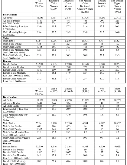
<Table 2.3>
Table 2.3 shows that both the IMR and the CMR differed between the social groups (defined
earlier in the chapter) with mothers from the Scheduled Tribes (ST) and the Scheduled Castes (SC)
recording the highest IMR and CMR – respectively, 14.3 and 17.5 for IMR and 33.2 and 33.9 for
CMR - and mothers from the non-Muslim Upper Classes (NMUC) recording the lowest IMR and
CMR of, respectively, 10.1 and 16.0. Table 2.3 also pointed to a gender bias in infant and child
mortality with both the IMR and the CMR being lower for male, than for female, births, with none of
the social groups being exempt from this bias: for the 36,794 mothers in their entirety, the male and
female IMR were, respectively, 12.1 and 14.1 while the male and female CMR were 22.8 and 28.2,
respectively.
In order to capture the regional dimension to infant and child deaths, the sample was
subdivided by mothers living in: the North (comprising the states of Jammu & Kashmir, Delhi,
Haryana, Himachal Pradesh, Punjab (including Chandigarh), and Uttarakhand); the Centre (Bihar,
Chhattisgarh, Madhya Pradesh, Jharkhand, Rajasthan, and Uttar Pradesh); the East (Assam, Orissa,
West Bengal); the West (Gujarat and Maharashtra); and the South (Andhra Pradesh, Karnataka,
Kerala, and Tamil Nadu). Table 2.3 shows that the IMR was lowest in the West and the South
(respectively, 3.9 and 5.1) and highest in the Centre (20.9) and, in similar vein, the CMR was lowest
in the West and the South (respectively, 8.8 and 8.1) and highest in the Centre (43.0)
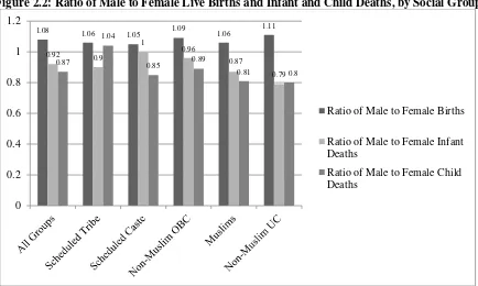
<Figures 2 and 3>
Figure 2 shows that the number of male births exceeded the number of female births: the
all-India ratio of the number of male to female births was 1.08 and this ratio was greater than one for
every social group. On the other hand, Figure 2 also shows that the number of male infant and child
deaths was smaller than the corresponding number of female deaths: the all-India ratio of the number
of male to female infant deaths was 0.92 and the ratio of the number of male to female child deaths
22 The IMR for India in 2013 was 40 (per 1,000 births) and the CMR in 2012 was 52 (per 1,000 births) as
15
was 0.87. Furthermore, this gender disparity in infant and child deaths was particularly marked for
the NMOBC, Muslims, and the NMUC. Figure 3 shows that the ratio of the number of male to
female births was greater than one for every region; however, when it came to infant and child deaths,
the number of male deaths was markedly smaller than that of female deaths in two regions, the North
and the Centre, but in the West and in the South the number of male infant and child deaths exceeded
the corresponding number for females.
In addition to the birth history file, the IHDS-2011 also had two further files which are
relevant to this study. The first was the Eligible Women’s file. The IHDS-2011 interviewed all
‘eligible’ women (EW) – that is ever-married women between the ages of 15 and 49 – from every
household and the eligible women’s file contained fairly detailed information on the circumstances
(both demographic and household), attitudes, and beliefs of these women and the constraints that they
faced within their households in terms of their autonomy of action, in particular with respect of their
children. Of these 39,523 EW, 2,729 did not have any children and hence were excluded from the
birth history file.
The third file in IHDS-2011 related to the household – inter alia its social group, its location,
its state of residence, the highest educational level of its adult males and females, its monthly per
capita consumption, its location (rural, urban), its state of residence. Merging the birth history file
with the EW and the household files yielded information for the 36,794 mothers on (i) their birth
history (from the birth history file); (ii) on their circumstances, attitudes, beliefs, and degree of
autonomy (from the EW file); and (iii) on their household circumstances (from the household file).
2.6 Estimation of the Infant and Child Mortality Equations
Suppose there areN (live) births (indexed i=1…N) to M mothers (indexed j=1…M) such that
the dependent variable, y takes the value 1 if the condition is present (birth i results in an infant or
child death: yi=1) and the value 0 if the condition is absent (birth i survives through infancy or
childhood:yi=0). If Pr[yi=1] and Pr[yi=0] represent, respectively, the probabilities of an infant
16
function of K variables (indexed k=1…K) which take values, X Xi1, i2...XiK with respect to birth i,
i=1…N:
1
Pr[ 1]
log
1 Pr[ 1]
K i
k ik i i k
i
y
X u Z
y = β
= = + =
− =
∑
(2.1)where: βk is the coefficient associated with variable k, k=1…K.
From equation (2.1) it follows that:
ˆ ˆ 1 Pr[ 1] 1 i i i i z X
i z X
e e e y e β β + = = =
+ (2.2)
where, the term ‘e’, in the above equation represents the exponential term.
A novel feature of the estimation was that the gender variable was allowed to interact,
separately, with the birth order of the child, the social group variable, and with the regional variable.
This allowed the probability of gender bias in infant and child deaths to be different between the birth
orders, the social groups and between the regions. To appreciate the difference between an
‘interacted’ and a ‘non-interacted’ equation consider the following equations for a variable Y which is
explained by two explanatory variables X and Z, for observations indexed i=1…N, without and with
interaction between X and R.
(
)
i i i
i i i i i
Y X R
Y X R X R
α β γ
α β γ φ
= + +
= + + + × (2.3)
In the first equation of equation (2.3) - without the interaction termXi×Ri - the marginal
change in Yi, given a small change in the value of the variable Xi , is β: the marginal effect, ∂ ∂Yi Xi
, is independent of the value of the variable Ri . In the second equation - with the interaction term
i i
X ×R - the marginal change in Yi, given a small change in the value of the variable Xi , is β φ+ Ri:
the marginal effect,∂ ∂Yi Xi, depends on the value of the variable Ri . If interaction effects are
significant then an equation which neglects them would be under specified.
The logit estimates showed that, for infant deaths, two of the three possible interactions
between sex at birth and birth order, one of the four possible interactions between sex at birth and a
17
household’s region of residence, were significantly different from zero. For child deaths, all three
possible interactions between sex at birth and birth order, one of the four possible interactions
between sex at birth and a household’s social group, and three of the four possible interactions
between sex at birth and a household’s region of residence, were significantly different from zero.
Taken together, these results implied that, had these interactions been neglected, the infant and child
mortality equations would have been under-specified.
<Tables 2.4 and 2.5>
However, the logit estimates, that is the βk of equation (2.1), themselves do not have a natural
interpretation – they exist mainly as a basis for computing more meaningful statistics and the most
useful of these are the predicted probabilities (of infant deaths) defined by equation (2.2).
Consequently, as Long and Freese (2014) suggested, results from the estimated equation were
computed, from the estimated logit coefficients of the infant and child mortality equations, as the
predicted probabilities of, respectively, infant and child deaths. These are shown in Table 2.4 as the
predicted infant mortality rate (PIMR), defined as predicted infant deaths per 1,000 births, and in
Table 2.5, as the predicted child mortality rate (PCMR), defined as predicted child deaths per 1,000
births.23
The PIMR and PCMR associated with births in the different variable groups shown in Tables
2.4 and 2.5, respectively, were computed through a series of simulations. The PIMR and PCMR of
male births was computed by first assuming that all the 108,517 births were male but with their
non-gender attributes – birth order, region, location, highest education of household adult, consumption
quintile, mothers’ health status – unchanged at observed values. Then the male coefficient was
applied to this synthetic sample of 108,517 male births in order to compute the male PIMR, shown in
Table 2.4 as 12.4 infant deaths per 1,000 births, and the male PCMR, shown in Table 2.5 as 23.5 child
deaths per 1,000 births.
The female PIMR and PCMR were computed similarly but this time assuming that all the
108,517 births were female, with non-gender attributes as observed. Applying the female coefficients
23 For example a predicted probability of 0.4 of an infant death translated as a predicted IMR of 40 per 1,000
18
to this synthetic sample of 108,517 female births, the female PIMR was 14.2 infant deaths per 1,000
births (Table 2.4) and the female PCMR was 28.5 child deaths per 1,000 births (Table 2.5). Since the
only difference between the male and female ‘synthetic’ samples was the gender at birth, the
difference between the two PIMR (12.4 and 14.2) and between the two PCMR (23.5 and 28.5) could
be attributed entirely to gender difference.24
The marginal PIMR and PCMR, shown in column 3 of Tables 2.4 and 2.5 represent,
respectively, the differences between the PIMR and the PCMR of the category in question and that of
the reference category. For example, in the gender grouping, males are the reference category and the
value of 1.8 in column 3 of Table 2.4 is the difference between the female (14.2) and male (12.4)
PIMR; similarly, the value of 5.0 in column 3 of Table 2.5 is the difference between the female (28.5)
and male (23.5) PCMR. Dividing these marginal PIMR and PCMR by their standard errors yields
their respective z-values (column 4 of Tables 2.4 and 2.5); these show whether the marginal PIMR
and PCMR were significantly different from zero in the sense that the likelihood of observing these
values, under the null hypothesis of no difference was (as shown by the p-values in column 5 of
Tables 2.4 and 2.5) greater or less than 5 (or 10) percent. The difference between the female-male
PIMR and between the male-female PCMR were, with z-values of 2.7 (Table 2.4) and 5.2 (Table 2.5),
significantly different from zero.
Table 2.4 also shows that, with the NMUC as the reference group, it was only the PIMR of
the Scheduled Tribes (ST) and the Scheduled Castes (SC) that were significantly higher than the
PIMR of the reference group of the non-Muslim Upper Classes (NMUC); the PIMR of the other
groups –the non-Muslim OBC and Muslims - were not significantly different from that of the NMUC.
In the context of child mortality, Table 2.5 shows the PCMR of the ST, the SC, and Muslims were
significantly higher than the PCMR of the reference group of the NMUC while the PCMR of the
NMOBC was not significantly different from that of the NMUC.
In terms of regions, the estimates, shown in Tables 2.4 and 2.5, suggest that the PIMR and
PCMR were lowest in the West (respectively, 4.2 and 9.9) and in the South (respectively, 5.2 and 8.4)
24 In computing these probabilities, all the interactions between gender and social group and gender and region
19
and highest in the Centre (respectively, 20.2 and 40.7). With the North as the reference region, both
the PIMR and PCMR were significantly lower in the East, the West, and the South and significantly
higher in the Centre (column 3 of Tables 2.4 and 2.5).
The highest level of education of a household adult significantly affected the chances of both
infant and child survival. As Tables 2.4 and 2.5 show, both the PIMR and PCMR fell for successively
higher education levels from highs of 16.6 (PIMR) and 33.2 (PCMR) when no adult in a household
had any education to lows of 7.6 (PIMR) and 14.1 (PCMR) when at least one of the household adults
was a graduate. After controlling for education, monthly per-capita household consumption
expenditure (HPCE) did not exercise a significant influence on infant and child mortality except,
perhaps surprisingly, the PIMR and PCMR were lowest for births in the lowest decile of HPCE
compared to births in the higher deciles. Lastly, as Tables 2.4 and 2.5 show, the state of a mother’s
health exercised a significant influence on the (predicted) survival chances of her infants and children:
the PIMR and PCMR were significant lower for mothers in good to fair health compared to those in
poor to very poor health.
Gender Bias in Infant and Child Deaths
The issue of the PIMR and PCMR, discussed above in the context of Tables 2.4 and 2.5, is
separate from whether the PIMR and PCMR were significantly different between male and female
births: underlying a low PIMR and PCMR might be significant differences between the predicted
survival chances of male and female births while, on the other hand, a high PIMR and PCMR might
go hand-in-hand with an absence of gender bias. Since, in the estimated equations, the sex at birth
variable was allowed to interact with the birth order, the social group, and the regional variable, it is
possible to test, in respect of these three variables whether the PIMR and the PCMR were
significantly different between male and female births. The results of these tests are shown in Tables
2.6 and 2.7. The second and third columns of Tables 2.6 and 2.7 show, respectively, the male and
20
PCMR (Table 2.7) while the fourth column in each Table shows the z-values associated with these
differences.25
<Tables 2.6 and 2.7>
These show that the PIMR and PCMR were not significantly different for the first birth: the
z-values associated with the male-difference of 0.7 in the PIMR, and 1.3 the PCMR, of the first birth
were, respectively, 0.6 (Table 2.6) and 0.7 (Table 2.7). However, for the second birth onwards, the
female PCMR was significant higher than the male PCMR and, for the fourth (and higher) birth, the
female PIMR, too, was significant higher than the male PIMR.
In terms of social groups, it was only for the non-Hindu OBC (NMOBC) and the non-Hindu
Upper Classes (NMUC) that the female PIMR was higher than the male PIMR; for the other three
groups – the ST, the SC, and Muslims – there was no significant difference between the male and
female PIMR. Gender bias in child mortality rates (shown in Table 2.7), however, existed in all the
social groups, with the exception of the ST, with the PCMR for males being significantly lower than
for females among the SC, the NMOBC, Muslims, and the NMUC.
In terms of the regions, it was only for the North and the Centre that there was clear evidence
of gender bias in male and female survivals. The male PIMR and PCMR for the North was, at 10.4
and17.7, respectively, significantly lower than its female PIMR and PCMR of 15.5 and 26.0,
respectively; for the Centre, the male PIMR and PCMR of 19.0 and 36.8, respectively, were both
significantly lower than its female PIMR and PCMR of 21.6 and 44.9, respectively. There was no
significant difference between male and female PIMR, and between male and female PCMR, for the
East and for the West. For the South, the gender bias in mortality rates was reversed with the male
PIMR and PCMR significantly exceeding their female counterparts.
The fact that the predicted survival probabilities of male infants and male children being
greater than that of their female counterparts is due to “son preference” among households in India.
As Borooah and Iyer (2005) point out, one way to think about this is that just as sons bring ‘benefits’
to their parents, daughters impose ‘costs’. Complementing a desire to have sons is a desire not to
25 The fifth column of Tables 2.6 and 2.7 shows the probability of exceeding the observed z-value on the null
21
have daughters so that the desire for sons tends to increase family size while the fear of daughters
limits it. The evidence from IHDS-2011 is that women whose first child was a son had, on average,
fewer births than women whose first child was a daughter (2.9 compared to 3.1) and that women
whose first and second children were sons had, on average, fewer births than women whose first and
second children were daughters. This suggests that the desire for sons and the fear of daughters
operate in sequence to limit family size: first the family tries to have sons and this expands family size
but, once this has been achieved, the fear of daughters limits family size.
2.7 Conclusions
This chapter investigated whether there was a social gradient to health in India with respect to
two health outcomes: the age at death and the rates of infant and child mortality per 1,000 live births.
In terms of age at death, the evidence suggested that the age at death was significantly higher in
households living in a forward state (compared to living in a backward state) and was significantly
lower in labourer (compared to non-labourer) households. The age at death in households was
significantly affected by their living conditions: in particular, in both the 71st and the 60th rounds, the
age at death was significantly lower in households that used fossil fuel for cooking instead of gas or
electricity and, in the 70th round, the age at death was significantly lower in households which did not
have a flushable toilet.
However, even after controlling for these “group independent” factors, the social group to
which people in India belonged had a significant effect on their health outcomes. Compared to
households from the non-Muslin Upper Classes, the predicted age at death in India in 2014 – after
imposing all the controls - was nearly eight years lower for ST households, nearly 13 years lower for
SC households, 5 years lower for non-Muslim OBC households, and nearly three years lower for
Muslim households. Notwithstanding the fact that in the decade between 2004 and 2014, the
predicted age at death rose for all the groups, inter-group disparities in the age at death remained
stubbornly durable.
There can be little doubt, therefore, that, on the basis of data from the NSS samples, the
analysis in this chapter offered prima facie evidence of a social group bias to health outcomes in
22
there are important health-related attributes of individuals (smoking, diet, taking exercise, the nature
of work) which are not - and, indeed, given the limitations of the data, cannot – be taken account of.
All these factors are included in the package of factors termed “unobservable”. If these unobservable
factors were randomly distributed among the population this, in itself, would not pose a problem.
However, there is evidence that there may be a group bias with respect to at least some of these
factors. For example, if hard physical work is more inimical to health than sedentary jobs, then of
males aged 25-44 years, 42 percent of ST and 47 percent of SC, compared to only 10 percent of
persons from the non-Muslim Upper Class, worked as casual labourers (Borooah et. al. 2007).
There is a natural distinction between inequality and inequity in the analysis of health outcomes.
Inequality reflects the totality of differences between persons, regardless of the source of these
differences and, in particular, regardless of whether or not these sources stem from actions within
a person's control. Inequity reflects that part of inequality that is generated by factors outside a
person's control. In a fundamental sense, therefore, while inequality may not be seen as
“unfair”, inequity is properly regarded as being unfair. The point about group membership is
that while it may not be the primary factor behind health inequality, it is the main cause of health
inequity. This chapter's central message, conditional on the caveats noted earlier, is that
belonging to the ST, the SC, or being Muslim in India seriously impaired, using the
language of Sen (1992), the capabilities of persons to function in society.
The findings with respect to infant and child deaths is that it was only the predicted IMR for
the Scheduled Castes that was significantly higher than that for the reference category of non-Muslim
Upper Classes with the predicted IMR for the other social groups not significantly different from the
that of the reference group. The contours of a social gradient to mortality begin to emerge, however,
with respect to child deaths: now the predicted CMR for three groups - the Scheduled Tribes, the
Scheduled Castes, and Muslims – were all significantly higher than that for the reference category of
non-Muslim Upper Classes.
However, the overriding worry with respect to infant and child mortality is gender bias with
23
study has shown, gender bias in infant and child mortality rates is, with stray exceptions26, a feature of
all the social groups. In addition, there is significant gender bias in favour of boys in two – the North
and the Centre - of the five regions of this study. At least part of this excess mortality stems from the
neglect of the girl child and, as Borooah (2004) showed, some of this neglect stemmed from the
inferior diet offered to girls compared to boys and from parental laxity in fully immunising their
daughters compared to their sons. In this context, the Indian Prime Minister, Narendra Modi’s call to
“Beti Bachao” (save a daughter) acquires a special urgency.
24 References
Birdi, K., Warr, P., and Oswald, A. (1995), “Age Differences in Three Components of
Employee Well-Being,” Applied Psychology, 44: 345-73.
Black, D, Morris, J., Smith, C. and Townsend, P. (1980), Inequalities in Health: A Report of a
Research Working Group, London: Department of Health and Social Security.
Bongaarts, J. and Guilmoto, C. Z. (2015), “How Many More Missing Women? Excess
Female Mortality and Prenatal Sex Selection, 1970–2050”, Population and Development Review,
41: 241–269.
Borooah, V.K. (2000), “The Welfare of Children in Central India: Econometric Analysis and
Policy Simulation”, Oxford Development Studies, 28: pp. 263-87.
Borooah, V.K. (2003), “Births, Infants and Children: an Econometric Portrait of Women and
Children in India”, Development and Change, 34: 67-103.
Borooah, V.K. (2004), “Gender Bias among Children in India in their Diet and Immunisation
Against Disease”, Social Science and Medicine vol. 58, pp. 1719-1731.
Borooah, V.K. and Iyer, S. (2005), “Religion, Literacy, and the Female-to-Male Ratio”,
Economic and Political Weekly, 60: 419-428.
Borooah, V.K, Dubey, A., and Iyer, S. (2007), “The Effectiveness of Jobs Reservation: Caste,
Religion, and Economic Status in India”, Development & Change, 38: 423-455.
Brunner, E. and Marmot, M., (1999), “Social Organisation, Stress and Health”, in M. Marmot
and R. Wilkinson (eds), The Social Determinants of Health, New York: Oxford University Press, pp.
17-43.
Caldwell, J.C. (1979), “Education as a Factor in Mortality Decline: an Examination of
Nigerian Data”, Population Studies, 33: 395-413.
Caldwell, J.C. (1986), “Routes to Low Mortality in Poor Countries”, Population and
Development Review, vol. 12, pp. 171-220.
Desai, S., Dubey, A., and Vanneman, R. (2015). India Human Development Survey-II
University of Maryland and National Council of Applied Economic Research, New Delhi. Ann Arbor,
25
Dreze, J. and Sen, A.K. (1996), Economic Development and Social Opportunity, New Delhi:
Oxford University Press.
Epstein, H. (1998), “Life and Death on the Social Ladder”, The New York Review of Books,
XLV: 26-30.
Griffin, J.M., Fuhrer, R., Stansfeld, S.A., and Marmot, M. (2002), “The Importance of Low
Control at Work and Home on Depression and Anxiety: Do These Effects Vary by Gender and Social
Class, Social Science and Medicine, 54: 783-98.
Guha, R. (2007), “Adivasis, Naxalities, and Indian Democracy”, Economic and Political
Weekly, XLII: 3305-3312.
Hobcraft, J. (1993), “Women’s Education, Child Welfare and Child Survival: A Review of
the Evidence”, Health Transition Review, 3: 159-173.
Karasek, R., Marmot, M. (1996), “Refining Social Class: Psychosocial Job Factors”, chapter
presented at The Fourth International Congress of Behavioral Medicine, Washington, D.C., March
13-16.
León-Cava, N., Lutter, C., Ross, J. Martin, L. (2002), Quantifying the Benefits of Breast
Feeding: A summary of the Evidence, Washington D.C: Pan American Health Organization.
Long, J.S., and Freese, J. (2014), Regression Models for Categorical Dependent Variables
using Stata, Stata Press: College Station, Tx.
Marmot, M. (1986), “Does Stress Cause Heart Attacks”. Postgraduate Medical Journal, 62:
683-686.
Marmot, M. (2000), “Multilevel Approaches to Understanding Social Determinants”, in L.
Berkman and I. Kawachi (eds), Social Epidemiology, Oxford University Press: New York, pp.
349-367.
Marmot, M. (2004), Status Syndrome: How Our Position on the Social Gradient Affects
Longevity and Health, London: Bloomsbury Publishing.
Murthi, M., Guio, A-C, and Dreze, J. (1995), “Mortality, Fertility and Gender Bias in India”,
26
Mustafa, H.E. and Odimmegwu, C. (2008), “Socioeconomic Determinants of Infant
Mortality in Kenya: Analysis of Kenya DHS 2003”, Journal of Humanities and Social Sciences, 2:
1-16.
Parikh, K. and Gupta ,C. (2001), “How Effective is Female Literacy in Reducing Fertility?”,
Economic and Political Weekly, XXXVI: 3391-98.
Puffner, R.R. and Serrano, C.V. (1975), Birthweight, Maternal Age, and Birth Order: Three
Important Determinants of Infant Mortality, Scientific Publication No 294, Washington D.C.: Pan
American Health Organization.
Sen, A.K. (2001), ‘The Many Faces of Gender Inequality’. Frontline, 18: October 27- 9
November.
Sen, G., Iyer, A., and George, A. (2007), “Systematic Hierarchies and Systemic Failures:
Gender and Health Inequalities in Koppal District”, Economic and Political Weekly, XLII: 682-690.
Sengupta, J., Sarkar, D. (2007), “Discrimination in Ethnically Fragmented Localities”,
Economic and Political Weekly, XLII: 3313-3322.
Subbarao, K. and Rainey, L. (1992), Social Gains from Female Education: a Cross-National
Study, Policy Research Working Chapters WPS 1045, Population and Human Resources Department,
Washington, DC: World Bank.
Tendulkar, S. (2007), “National Sample Surveys” in K. Basu (ed), The Oxford Companion to
Economics in India, New Delhi: Oxford University Press, pp. 367-370.
Theil, H. (1954), Linear Aggregation of Economic Relations, North Holland: Amsterdam.
Trivedi, A. and Timmons, H. (2013), “India’s Man Problem”, The New York
Times, https://india.blogs.nytimes.com/2013/01/16/indias-man-problem/?_r=0&login=email (accessed
18 May 2017).
Wilkinson, R.G. and Marmot, M. (1998), Social Determinants of Health: The Solid Facts,
World Health Organisation: Copenhagen.
Woodbury, R.M. (1925), Causal Factors in Infant Mortality: a Statistical Study Based on
Investigations in Eight Cities, Children’s Bureau Publications No 142, Washington D.C.: Government
28 Figure 2.1
Mean Age at Death (Years) in India by Social Group
Source: NSS 60th and 71st NSS, Health File
44.6 43.3 49.7 43.6 54.5 48.3
49.5 46
55.3
59.4
63.2
54.8
0 20 40 60 80 100 120 140
Scheduled Tribe
Scheduled Caste
Non-Muslim Other Backward
Classes
Muslim Non-Muslim Upper Classes
All
2014 (71st NSS)
29
Table 2.1: Predicted Age at Death from Regression Equations, 71st and 60th NSS Round
71st NSS (2014)+
Conditioning Variable Age at Death Marginal Change Standard error
of marginal change
t value Pr>|t|
By gender of deceased
Male 53.6
Female 56.4 2.8 0.271 10.3** 0.00
By Social Group of Household
Scheduled Tribe 52.6 -7.9 0.547 -14.5** 0.00
Scheduled Caste 48.0 -12.5 0.455 -27.4** 0.00
Non-Muslim OBC 55.2 -5.2 0.394 -13.3** 0.00
Muslims 58.0 -2.5 0.469 -5.3** 0.00
Non-Muslim Upper Class [R] 60.5
Household Occupation
Labourer Household [R] 54.3
Non-Labourer Household 54.9 0.6 0.339 1.8* 0.07
Household’s Location
Rural[R] 54.7
Urban 55.0 0.3 0.368 0.8 0.40
Household’s State of Residence
Forward State [R] 57.7
Backward State 51.4 -6.3 0.282 -22.3** 0.00
Household Living Conditions: Latrine
Flush or Septic Tank [R] 55.3
Other Type of Latrine (including no latrine) 54.0 1.3 0.359 3.6** 0.00
Household Living Conditions: Cooking Fuel
Gas, Gobar Gas, Electricity, Kerosene [R] 56.4
Other Fuels 54.0 -2.4 0.383 -6.2** 0.00
Household Per-Capita Consumption Quintile
Lowest quintile 49.4 -9.5 0.500 -19.1** 0.00
2nd quintile 58.4 -0.6 0.468 -1.2 0.22
3rd quintile 51.8 -7.1 0.504 -14.1** 0.00
4th quintile 55.1 -3.9 0.469 -8.3** 0.00
30 Table 2.1 (continued)
60th NSS (2004)++
Conditioning Variable Age at Death Marginal Change Standard error
of marginal change
t value Pr>|t|
By gender of deceased
Male 48.6
Female 47.3 -1.301 0.3 -4.11** 0.00
By Social Group of Household
Scheduled Tribe 48.5 -1.8 0.663 -2.7** 0.01
Scheduled Caste 46.1 -4.1 0.507 -8.2** 0.00
Non-Muslim OBC 49.1 -1.2 0.429 -2.8** 0.01
Muslims 43.8 -6.5 0.569 -11.4** 0.00
Non-Muslim Upper Class [R] 50.3
Household Occupation
Labourer Household [R] 42.6
Non-Labourer Household 50.6 8.0 0.376 21.3** 0.00
Household’s Location
Rural [R] 48.6
Urban 46.3 -2.3 0.442 -5.3** 0.00
Household’s State of Residence
Forward State [R] 51.2
Backward State 44.6 -6.6 0.327 -20.1** 0.00
Household Living Conditions: Latrine
Flush or Septic Tank [R] 49.2
Other Type of Latrine (including no latrine) 47.8 -1.5 0.501 -2.9** 0.00
Household Living Conditions: Cooking Fuel
Gas, Gobar Gas, Electricity, Kerosene [R] 52.9
Other Fuels 47.0 -5.9 0.546 -10.9**
Household Per-Capita Consumption Quintile
Lowest quintile 47.3 -2.4 0.588 -4.1** 0.00
2nd quintile 45.9 -3.8 0.583 -6.5** 0.00
3rd quintile 48.6 -1.1 0.565 -2.0** 0.05
4th quintile 50.0 0.3 0.561 0.5 0.64
Highest Quintile [R] 49.7
+Estimated on data for 2,384 households in which a death occurred in the 71st NSS, after grossing up ++Estimated on data for 1,708 households in which a death occurred in the 60th NSS, after grossing up.
[R] denotes the reference category.
** Significant at 5%; * significant at 10%.
[image:32.595.66.531.82.447.2]31
Table 2.2: Predicted Age at Death: Differences between the 71st and 60th Rounds
Age at Death 71st
Round
Age at Death 60th
Round
Difference Standard
Error of Difference
t-value Pr>|t|
By gender of deceased
Male 53.4 49.2 4.2 0.269 15.5** 0.00
Female 56.2 47.9 8.3 0.324 25.5** 0.00
By Social Group of Household
Scheduled Tribe 52.2 49.2 3.0 0.687 4.3** 0.00
Scheduled Caste 47.7 46.9 0.8 0.461 1.7* 0.09
Non-Muslim OBC 54.9 49.8 5.1 0.344 14.8** 0.00
Muslims 57.6 44.5 13.1 0.575 22.8** 0.00
Non-Muslim Upper Class 60.1 51.0 9.1 0.476 19.2** 0.00
Household Occupation
Labourer Household 54.1 42.8 11.3 0.429 26.3** 0.00
Non-Labourer Household 54.7 50.8 3.9 0.248 15.7** 0.00
Household’s Location
Rural 54.5 49.3 5.1 0.259 19.9** 0.00
Urban 54.8 47.0 7.8 0.470 16.6** 0.00
Household’s State of Residence
Forward State 57.5 51.8 5.7 0.291 19.7** 0.00
Backward State 51.2 45.2 6.0 0.311 19.3** 0.00
Household Living Conditions: Latrine
Flush or Septic Tank 54.9 48.3 6.7 0.272 24.5** 0.00
Other Type of Latrine (including no latrine)
53.6 49.7 3.9 0.482 8.1** 0.00
Household Living Conditions: Cooking Fuel
Gas, Gobar Gas, Electricity, Kerosene
56.3 53.1 3.2 0.530 6.1** 0.00
Other Fuels 53.9 47.1 6.8 0.270 25.2** 0.00
Household Per-Capita Consumption Quintile
Lowest quintile 49.4 48.0 1.4 0.443 3.2** 0.00
2nd quintile 58.4 46.6 11.8 0.414 28.4** 0.00
3rd quintile 51.8 49.3 2.5 0.497 5.1** 0.00
4th quintile 55.0 50.7 4.4 0.481 9.1** 0.00
Highest Quintile 58.9 50.4 8.5 0.586 14.5** 0.00
Estimated on data for 4,019 households in which a death occurred in the 71st and 60th Rounds. ** Significant at 5%; * significant at 10%.