Munich Personal RePEc Archive
The Unusual Trading Volume and
Earnings Surprises in China’s Market
Chong, Terence Tai Leung and Wu, Yueer
The Chinese University of Hong Kong
5 February 2018
Online at
https://mpra.ub.uni-muenchen.de/92162/
The Unusual Trading Volume and Earnings Surprises in China’s Market
CHONG, Terence Tai Leung
WU, Yueer
Department of Economics, The Chinese University of Hong Kong
5/2/2019
Abstract
This study examines the empirical relationship between unusual trading volume
and earnings surprises in China's A-share market. We provide evidence that an
unusually low trading volume contains negative information about firm fundamentals.
Moreover, unusual trading volumes could predict abnormal returns close to the
earnings announcement date. The degree of and changes in the divergence of opinion
could explain this result. Our study provides an insight into China's market, where
short sales are strictly forbidden. We report a strong relationship that is quite different
from that described in most studies on the United States market. The differences in
the findings are likely due to differences in the nature of the market, which is
consistent with Miller (1977).
I. Introduction
Gervais, Kaniel and Mingelgrin (2001) examined the relationship between
extreme trading activity and the evolution of stock prices. They found that unusually
high or low trading volumes, measured over a day or a week, are often followed by
relatively high or low stock returns. Inspired by this study, many other researchers
have examined the impacts of unusual trading volume, such as changes in visibility
and short-selling constraints. Most studies focused on stock markets in developed
countries, especially in the United States. However, there has been little
characterization of these trends in the Chinese market. This study explored the
relationship between unusual trading volume and earnings surprises for individual
stocks in China.
First, we empirically examined whether extreme trading activities play an
informational role to predict earnings surprises in China’s market. Unusually high and
low trading volume might indicate significant, unexpected earnings. In contrast to
what has been observed in the United States, stocks with unusually high trading
volume may experience lower returns, and those with unusually low trading volume
may experience higher returns close to the earnings announcement date in China. This
is because the high-volume return premium, a significant component of the United
States stock market, does not exist in China, which is a difference in the nature of the
market. Stocks that are subject to divergent opinions and short-selling constraints may
be biased upwards and thus experience negative return near an earnings
2
United States, stocks with unusually low trading volume prior to earnings
announcements may have relatively lower unexpected earnings in terms of standard
unexpected earnings (SUE). SUE is closely related to firm fundamentals, which can
be considered as cash flow. Unusually low trading volume indicates low divergence
of opinion and a consensus that there are relatively worse firm fundamentals because
under short-selling constraints, agents who are informed of bad news incline to avoid
trading. My findings suggest the drivers and the mechanisms of earnings surprises in
terms of cash flow and market expectations are different.
The ability of an unusually high trading volume to predict higher return is
similar in the stock markets of some developed countries, especially the United States.
Gervais, Kaniel and Mingelgrin (2001) used data from 1963 to 1996 to examine the
high-volume premium in the United States market. Chen, Firth and Rui (2001)
examined the markets of nine developed regions and found a positive correlation
between trading volume and stock price change from 1973 to 2000. Mayshar (1983)
postulated that holders of a specific stock are more optimistic about its prospects; an
unusually high volume suddenly would increase the visibility of the stock, leading to
higher demand from and price expectations of its holder.1 In China, however, an
unusually high trading volume signals a higher return, and unusually low trading
volume predicts a lower return. The opposite effect might suggest another explanation.
Banerjee and Kremer (2010) found that unusually high volume indicates a greater
divergence of opinion about stock prospects. Miller (1977) hypothesized that prices of
1
stocks without short-selling are biased upwards if there is high divergence of opinion.
Berkman, Dimitrov, Jain, Koch and Tice (2009) found that if earnings announcements
reduce differences of opinion and overvaluation; stocks with high difference of
opinion and stricter short-selling constraints often experience a decline in price
around the earnings announcement date. By the same logic, it could be deduced that if
the views about a stock with lower difference of opinion before the earnings
announcement become more divergent after the announcement, the stock tends to
have a higher excess return relative to the market close to the earnings announcement
date.
For unusually low trading volume, Diamond and Verrecchia (1987) argue that
prohibiting traders from short-selling increases the time needed for the market price to
adjust to private information, especially if it is bad news. Thus, under short-selling
constraints, the instantaneous price of a stock might not reflect the market expectation
of all agents. If some agents receive bad news, they may be inclined not to trade, thus
decreasing trading volume. Akbas (2016) invoked this argument and provided
evidence from the United States market that an unusually low trading volume signals
weak firm fundamentals. The negative relationship between an unusually low trading
volume and firm fundamentals becomes more significant for firms with severer
short-selling constraints.
Earnings announcements are scheduled regularly every quarter. The
management of the firm tries to convey relevant information about expected cash
4
earnings, quarterly announcements also provide substantial details that could help
investors acquire better understanding of the firm’s prospects. Thus, this information
could be used to examine whether any signal received prior to the announcement date
contains information about firm fundamentals.
The primary contribution of this study is to examine if an unusual trading
volume predicts earnings surprises in China’s market. We present evidence that an
unusually low trading volume predicts lower cash flow and a higher return, and an
unusually high trading volume predicts a lower return, which is partly different from
the relationship observed for the markets in the United States and most developed
countries. Additionally, we improve the existing methodology by using a fixed effect
regression to analyze panel data and focusing on each individual stock rather than
portfolios, making the results more reliable.
It is important to study the Chinese market for several reasons. First, the
Chinese equity market has expanded rapidly recently. From January 2000 to
December 2017, the number of stocks increased from 1,206 to 3,567, and the total
market capitalization has exceeded 8.7 trillion dollars. Since China’s stock market has
become an important part of the global economy and is incorporated into the global
capitalization market through Qualified Foreign Institutional Investor (QFII), insights
into the Chinese stock market may help global investors make better decisions.
There are strict short-selling constraints for the A-share market.2 Although there are a
few options for index futures, there are no futures or options for individual stocks.
Also, individual investors constitute the majority of market participants for China’s
stock market, but institutional investors are more prominent participants in the stock
market of the United States. This discrepancy in markets might lead to different
results.
The formal analysis of the relationship between unusual trading volume and
earnings surprises in China may reveal whether trading volume provides any
information about expected future returns in emerging markets. The rest of the paper
is organized as follows. Section 2 presents the methodology and the model. Section 3
describes the data set and the variables. Section 4 presents and analyzes the regression
results. Section 5 summarizes and presents the conclusions.
II. Methodology
Akbas (2016) started with the quarterly weighted Fama and MacBeth (1973)
regressions, in which the dependent variable is earnings surprises. In this method, the
cross-sectional coefficient of unusual trading volume is estimated for each quarter,
and then the weighted average of all coefficients is determined.3
, , , , , ,
(1)
2
Firms issue two types of shares: A-share and B-share. Class A shares are priced and traded in RMB and among Chinese citizens, while class B shares are traded in foreign currencies. Since the B-share stock market is much smaller than the A-share stock market, our study focuses on A-share stocks.
3
6
̅ ∑ (2)
In equation (1), i denotes each firm, and q refers to each quarter.
refers to surprises in earnings, measured by standard unexpected earnings (SUE) and
cumulative abnormal return (CAR). and are dummy variables,
denoting whether the trading volume of a firm i is unusually high or unusually low.
are other control variables which might influence the earnings surprises. In
equation (2), is the weight of estimator in quarter q, and ̅ is the weighted
average of all s.
Though this method could be used to study as many firms as possible, it only
considers the impact of time. In addition, the calculation of significance for the
weighted average estimator ̅ is based on the standard deviation of its distribution.
However, the standard deviation can only be calculated under the assumption that the
values of s in each interval are uncorrelated with each other, which cannot be
satisfied strictly.
To solve this problem, we performed a two-way fixed effect regression using
the panel data, fixing the time as well as the individuals. The model is the same as that
presented in equation (1). , is measured by the standardized unexpected
earnings, SUE, and the cumulative abnormal return, CAR, which is explained in the
next chapter.4
4
III. Data and Variables A. Sample
The main sample data, retrieved from the Wind Database, were for China’s
A-share stocks that were traded on the Shanghai Stock Exchange (SSE) and the
Shenzhen Stock Exchange (SZSE) between January 2008 and December 2017, over a
total of ten years. The use of a longer period causes the scale of the sample to shrink.
Moreover, this period includes a steady state (from March 2011 to July 2014), a
bullish period (from July 2014 to June 2015) and a bearish period (from June 2015 to
February 2016). The Wind Database is a reliable database widely used in the Chinese
financial industry. The trading interval of the data is a calendar quarter. Thus, there
are 40 intervals for the ten years of data. After removing stocks with missing data and
defining financial firms, about 1,200 stocks were selected for analysis. Since there
were only 1,494 listed companies in the A-share market until the end of 2007, the
fraction of coverage exceeded 78%, thereby roughly representing the majority of the
market.
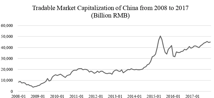
[image:9.612.115.485.514.685.2]
Figure 1 presents the trend of tradable market capitalization from January 2008 to 0
10,000 20,000 30,000 40,000 50,000 60,000
2008-01 2009-01 2010-01 2011-01 2012-01 2013-01 2014-01 2015-01 2016-01 2017-01 Tradable Market Capitalization of China from 2008 to 2017
8
December 2017.
Note: Average monthly data from the Wind Database are used.
B. Earnings Surprises
Following Akbas (2016), we have adopted two different methods to measure
earnings surprises: standardized unexpected earnings using historical accounting
information (SUE) and a stock’s cumulative abnormal return (CAR).5
Let i be each firm and q be each quarter. SUE is the unexpected earnings
divided by price, as specified in the following equation:
(3)
Unexpected earnings, , are constructed by a rolling seasonal random walk
(SRW) model: . In equation (3), EPS is the earnings per
share before extraordinary items are disclosed by the announcement of firm i during
quarter q. Livnat and Mendenhall (2006) also used the SRW model rather than a time
series model to measure earnings surprises. Next, is divided by to
obtain , the standardized unexpected earnings. is the price per share for
firm i at the end of the quarter q-4. This method has certain advantages. Since the
current price of a stock is positively correlated with future cash flows or earnings, this
method eliminates the impact of price. Second, most firms disclose EPS each quarter,
5
leading to a sufficiently large sample. Also, SUE directly reflects a firm’s
fundamental information, so that we can potentially obtain some information related
to future earnings prospects from the unusual trading volume.
To construct the cumulative abnormal return, CAR, we subtract the average
value-weighted market return, , from firm i’s average compounded stock return,
. The windows of market return and stock return are both a three-day interval
around the earnings announcement date. Let t be the earnings announcement date. It
should be noted that t of each quarter might differ from firm to firm. Thus, we first
calculate the daily CAR:
1 1 1 1 1 1
(4)
Once the daily CAR is calculated, the quarterly cumulative abnormal return,
, can be filtered from the daily time series, according to the time series
of earnings announcement dates of each firm. Compared with SUE, CAR
encompasses opinions about the price of the whole market. Thus, the regression
results might provide insight into better prediction of future price movements.
However, CAR also has limitations and can be affected by many factors other than
cash flow prospects.
C. Unusual trading volume
10
formation period and that of a reference period to determine if a firm should be
marked as a high-volume or a low-volume stock for the United States market. Lo and
Wang (2000) argued that trading turnover, defined as shares traded divided by shares
outstanding of a company, is a better measure of trading behavior than share volume,
dollar volume, or other alternatives. Different from the onefold setting of formation
period and reference period, we tried different length and start dates of the two
periods to obtain different signals. A stock is categorized as a high-volume or a
low-volume stock, depending on whether the average daily turnover of the formation
period of the stock exceeds a certain benchmark. Dummy variables, and
, will be assigned the value 1 if a firm falls into the high-volume group or the
low-volume group, respectively, otherwise it will be assigned 0. Using dummy
variables rather than continuous variables enables us to separately measure the
unusually high trading volume and unusually low trading volume. This method is also
more sensitive to the thick tail of the turnover distribution.
Table I
Parameters Value
Formation Period [-6, -2]
Reference Period [-61, -12]
Threshold for D_HIGH Top 20%
Threshold for D_LOW Bottom 20%
Table I displays the original parameters of D_HIGH and D_LOW, with the
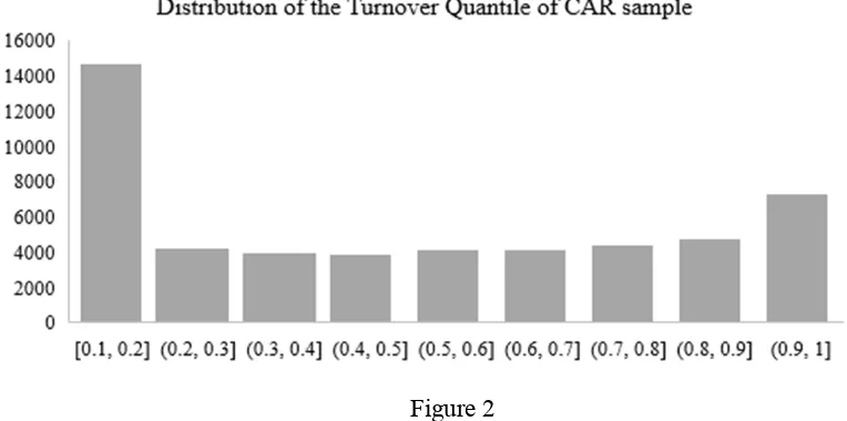
Figure 2
In Figure 2, QTL is the quantile of average daily turnover of the formation
period in the time series of average daily turnover of the reference period. Figure 2
shows the thick-tail property of turnover quantiles, confirming the need to use
D_HIGH and D_LOW instead of QTL.
D. Other Control Variables
Many studies have found that the size of a firm influences its market return
(Banz, 1981; Fama and French, 1992). Thus, a firm’s market equity (ME), which is
the price multiplied by outstanding shares, is included in this analysis. Also, the ratio
of a firm’s previous quarter-end book value of common equity (BE) to its market
equity (ME) is considered. Logged ME and BM values are used to avoid the
skewness of their distributions, and firms with negative BE are excluded. Following
12
return of the reference period ([-61, -12]) and the formation period ([-6, -2])6 right
before the earnings announcement date, respectively. IVOL, the standard deviation of
daily return over the 10-day period [-11, -2], is also included. Next, following
Nofsinger and Sias (1999), we identified a strong positive correlation between
institutional ownership and stock returns. Thus, IO, the ratio of the firm’s institutional
ownership, is considered. If a firm has an occasionally missing IO but has previously
reported the values before and after the gap, we fill in the missing information with a
linearly interpolated IO value. TURNR, the average turnover over the reference
period [-61, -12], is also included. Finally, the earnings surprise in the previous
interval is incorporated and marked with LAG.
E. Divergence of Opinion Measures
Berkman et al. (2009) used three proxies to measure difference of opinion,
DISP, RETVOL, and TURN. DISP is the standard deviation of analysts’ forecasts of
EPS. However, the analysis of EPS in the Wind Database is updated only yearly for
the annual report, and these records are also incomplete. Thus, DISP is not considered
in this analysis, but the other two proxies, RETVOL and TURN, are used. RETVOL
is the standard deviation of the excess daily return relative to the market return around
the earnings announcement date. TURN is the average daily turnover surrounding a
quarterly announcement. RETVOL and TURN reflect direct information about the
6
divergence of opinion of market participants, since the price and the quantity of
equity reflect the valuation of all agents.
IV. Estimation A. Summary Statistics
We constructed two subsamples, the SUE sample and the CAR sample,
according to the method employed to measure earnings surprises. The two
subsamples extend from the start of 2008 to the end of 2017, giving a total of 40
quarters. The SUE sample includes 1,180 A-share stocks, with 47,200 observations in
total. The CAR sample includes 1,283 A-share stocks, with 51,320 observations in
total. This difference in the number of observations is because of the fact that some
firms do not release earnings announcements every season, which results in missing
SUE data. We next excluded firms that fell into the categories of “Banks” and
“Non-bank Financials” according to the SWS industry classification.7 To calculate
the panel data statistics, we obtained cross-sectional statistics of each quarter and took
the time-series average. The crucial independent variables, D_HIGH and D_LOW,
are included but not presented in the table because they are dummy variables. In these
two samples, the formation period is [-5, -1], and the reference period is [-55, -6]. If
the average daily turnover of the formation period exceeds the 80th quantile of the
average daily turnover time series of the 10-week reference period, D_HIGH is
7
14
marked as 1. If the average daily turnover of the formation period is less than the 20th
quantile of the reference period, D_LOW is marked as 1.8
Table II
Panel A: SUE Sample
Sample Period: 2008 Q1 - 2017 Q4 (40 Quarters)
Number of Stocks: 1,180
Number of Observations: 47,200
Mean Median STD Min P_25 P_75 Max
SUE 0.125% 0.036% 3.239% -29.942% -0.639% 0.695% 37.922%
logSIZE 22.216 22.072 0.897 20.077 21.572 22.711 26.741
logBM -1.420 -1.409 0.861 -4.742 -2.003 -0.814 1.760
IO 40.448 40.027 20.059 0.107 25.606 54.901 100.268
RETR 3.964% 2.038% 17.195% -54.326% -6.146% 11.900% 141.015%
RETF -0.186% -0.384% 5.965% -34.086% -3.831% 3.047% 35.725%
TURNR 0.021 0.018 0.016 0.000 0.012 0.027 0.140
IVOL 0.448 0.312 0.531 0.000 0.180 0.539 8.051
QTL 0.529 0.510 0.305 0.100 0.268 0.790 1.000
8 Akbas (2016) uses 20% as the threshold to determine D_HIGH and D_LOW values; Gervais, Kaniel and Mingelgrin (2001) use 10% as the threshold.
Panel B: CAR Sample
Sample Period: 2008 Q1 -2017 Q4(40 Quarters)
Number of Stocks: 1,283
Number of Observations: 51,320
Mean Median STD Min P_25 P_75 Max
CAR -0.090% -0.159% 1.589% -11.670% -0.942% 0.671% 9.084%
logSIZE 22.197 22.044 0.927 20.053 21.542 22.697 27.480
logBM -1.453 -1.464 0.870 -4.742 -2.047 -0.843 1.980
IO 40.207 39.884 20.541 0.095 25.103 54.989 106.409
RETR 3.896% 1.972% 17.255% -55.876% -6.231% 11.892% 143.811%
RETF -0.204% -0.402% 6.003% -35.539% -3.838% 3.022% 36.298%
TURNR 0.022 0.018 0.016 0.000 0.012 0.028 0.149
IVOL 0.458 0.318 0.545 0.000 0.183 0.553 8.254
[image:17.612.112.504.179.405.2]QTL 0.527 0.510 0.305 0.100 0.260 0.790 1.000
Table II presents the time-series averages of summary statistics of dependent
and independent variables in each quarter. Panel A describes the SUE sample. SUE is
equal to the difference in EPS between quarter q and quarter q-4 divided by the price
per share in quarter q-4. It is presented in percentage form. Panel B shows the
statistics for the CAR sample. CAR is defined as the average compounded return of
the stock around the earnings announcement date subtracted by that of the market.
Both samples span 10 years, 40 quarters from 2008 Q1 to 2017 Q4. CAR is also
presented in percentage form. Other control variables are also included in both panels.
To determine logSIZE, we multiplied the price per share by the share number. logBM
is the log of the ratio of the book value to the equity market value. Defining the
16
-12] as RETR and the stock return over the period [-6, -2] as RETF. These are both
presented as percentages. TURNR is the average turnover for the same period as
RETR. IVOL is the standard deviation of daily return over the period [-11, -2]. Since
D_HIGH and D_LOW are dummy variables, they are not included and are replaced
by QTL. QTL is the quantile of the average turnover of the formation period in the
average turnover of the reference period and is presented in percentage form.
All variables are quite similar except SUE and CAR. The mean of SUE is 0.125%
and that of CAR is -0.090%. This indicates that the two methods capture different
parts of the earnings surprises. SUE captures more information about firm
fundamentals, and CAR better reflects the opinions of market participants.
Moreover, the correlation between SUE and CAR is quite low. Since the stock
pool of the SUE sample is a subset of that of the CAR sample, we use the stock lists
of the SUE sample as the pool and calculate the correlation coefficients between SUE
and CAR. As observed in Table III, the correlation coefficient of the whole time
period is about 0.03, and the time-series average of the quarterly correlation
coefficients is 0.057. The low correlation suggests that the current cash flow might
not be an important factor for investors to determine the value of their stocks. This is
also different from the situation in the United States.9
9
Table III
Total Correlation Coefficient 0.0297
Time-series Average of Quarterly Correlation Coefficients 0.0570
B. Portfolio Analysis
RETVOL and TURN express differences of opinion of the market in the form
of price and relative quantity. The periods are the 10-day periods [-10, -1] prior to the
earnings announcement date. The correlation coefficients between the whole time
series of RETVOL, TURN, and QTL of stocks in the CAR sample are displayed in
Table IV.
Table IV
RETVOL TURN QTL
RETVOL 1 0.49 0.35
TURN 0.49 1 0.46
QTL 0.35 0.46 1
To further explore the relation between divergence of opinion and extreme
trading volume, stocks in the CAR sample are analyzed by portfolio type. In each
quarter, stocks fall into five categories, V1 to V5, according to QTL.10 All stocks
marked as D_HIGH fall into V5, and all stocks marked as D_LOW fall into V1.
10
18
∆ and ∆ represent the differences over period [1,10] and period [-10,
-1], reflecting the change in divergence of opinion close to the release of the earnings
announcement.
Panel A of Figure 3 shows a linear pattern. Stocks with higher QTL tend to
experience a higher degree of divergence of opinion than those with lower QTL. Both
trends of RETVOL and TURN substantiate the explanation that stocks with greater
divergence of opinion also tend to have higher volume.
Panel B provides additional support for this explanation. Opinions concerning
stocks with higher divergence of opinion would decline around the earnings
announcement date. However, stocks with a relatively lower difference of opinion
tend to experience a divergence of opinion around the earnings announcement date.
This pattern of divergence of opinion around the earnings announcement date
helps to explain the regression results of the CAR sample, the reason for the positive
signal of unusually low trading volume, and the negative signal of unusually high
[image:20.612.121.499.562.728.2]trading volume.
Figure 3
1.54 1.77
1.96 2.24
2.93 1.05 1.73 2.09 2.60 3.95 0 0.5 1 1.5 2 2.5 3 3.5 4 4.5
V1 V2 V3 V4 V5
Panel A: Average RETVOL and TURN in Turnover Quantiles
Figure 3 displays time-series averages of the measure for divergence of opinion
for portfolios. Stocks are classified into five groups to represent five intervals of
turnover quantiles. In panel A, RETVOL is the standard deviation of excess daily
return relative to the market return over the [-10, -1] window prior to the earnings
announcement date. TURN is the average daily turnover over the same period as
RETVOL. TURN and ∆ are multiplied by 100 in order to fall in the similar
range of RETVOL and ∆ . In panel B, ∆ is the difference between
the RETVOL over the [1, 10] window and the [-10, -1] window. We used the CAR
sample for this analysis, which includes 1,283 stocks and is larger and more complete
than the SUE sample.
C. Estimation
1. Regression for the CAR sample
In Table V, the dependent variable is CAR. Fixed effect regressions are
0.36
0.19
0.06
-0.12
-0.53 0.40
0.20
0.06
-0.17
-0.50 -0.6
-0.4 -0.2 0 0.2 0.4 0.6
V1 V2 V3 V4 V5
Panel B: Average Difference of RETVOL and TURN in Turnover Quantiles
20
performed. To present the results more clearly, CAR and CARlag values are
multiplied by 100 and denoted as CAR’ and CARlag’. RETR and RETF are
multiplied by 100 and denoted as RETR’ and RETF’. Linear transformation does not
change the results or the significance of the regressions. Both estimates of the
two-way fixed effect regression and the one-way fixed effect regression for D_HIGH
are negative and significant at the 1% level, while the estimates of the two-way fixed
effect regression and the one-way fixed effect regression for D_LOW are both
positive and significant at the 5% level.
This result is different from that predicted for the United States market and
refutes the explanation of visibility, which claims that an extremely high trading
volume would increase the visibility of the stock, leading to a rise in the stock
prospects of optimistic holders. However, the unusually high volume indicates a wide
divergence of opinion about the prospects of the stock. Due to short-sale constraints,
the prices of these stocks are upwardly biased according to Miller’s (1977) theory.
Therefore, stocks may experience negative return around the earnings announcement
date if the divergence of opinion subsides, which is the reason for the negative
coefficient of D_HIGH. Also, stocks with increased divergence of opinion experience
a positive return, which explains the positive coefficient of D_HIGH.
In conclusion, the results shown in Table V confirm that a change in the
difference of opinion leads to a movement in price close to the earnings
announcement date. In this process, an unusual trading volume indicates the degree of
reflected by cumulative abnormal return.
Table V
Unusual trading volume and CAR’
Two-Way Fixed Effect One-Way Fixed Effect
CAR’ CAR’
CARlag’ 0.037*** 0.062***
(0.0000) (0.0000)
logSIZE -27.401*** -4.453***
(0.0000) (0.0000)
logBM 1.838 2.608***
(0.3196) (0.0023)
D_HIGH -17.094*** -16.836***
(0.0000) (0.0000)
D_LOW 4.022** 3.512**
(0.0266) (0.0493)
IO 0.340*** 0.108**
(0.0000) (0.0103)
RETR’ -0.081* -0.119***
(0.0549) (0.0045)
RETF’ -0.541*** -0.490***
(0.0000) (0.0000)
TURNR -504.096*** -550.413***
(0.0000) (0.0000)
IVOL -1.056 -2.318*
(0.4504) (0.0675)
Adjusted R2 0.027 0.024
22
column represents the two-way fixed effect regression, fixing the time as well as the
individuals. The second column is the one-way fixed effect regression, fixing the time
only. CAR’ is computed by subtracting the average compounded return of the market
from that of the stock around the earnings announcement date and then multiplying
by 100. CARlag’ is the CAR’ value from the previous quarter. D_HIGH and D_LOW
are dummy variables. These variables are equal to 1 if the daily average turnover of
the formation period is in the top or bottom 20% of the 10-week daily average
turnover series, otherwise they are 0. The p-values are presented under the coefficient
estimates. *, **, and *** indicate statistical significance at the 10%, 5%, and 1%
levels, respectively.
2. Regression for the SUE sample
Similar to the regression performed on the CAR sample, SUE and SUElag are
multiplied by 100 and denoted as SUE’ and SUElag’. Also, RETR and RETF are
multiplied by 100 and denoted as RETR’ and RETF’. In the data presented in Table
VI, it is obvious that the coefficients of D_LOW are both negative. For both two-way
and one-way fixed effect regressions, this value is statistically significant at the 10%
level. Stocks with an unusually low trading volume ahead of the earnings
announcement date are prone to have lower standard unexpected earnings, which
means deteriorated cash flow quality. This effect was not explained by firm size,
volatility, or SUE in the previous quarter.
However, the coefficient of D_HIGH remains insignificant for stocks in
China’s market. This is the same finding as that of Ferhat (2016) for stocks in the
United States. The fact that high volume stocks do not play an informational role to
predict surprises in a firm’s cash flows could be explained by high divergence of
opinion. Market participants have different expectations of stock prospects, so
unusually high trading volume does not have strong predictive power.
D_LOW is accompanied by less divergence of opinion and a consensus about
relatively lower standard unexpected earnings. Thus, it could be concluded that
unusually low trading volume contains unfavorable information about the future cash
flow of the stock. However, after the EPS of a specific quarter is disclosed, the market
digests this piece of information, and there may be an overshoot of the stock price,
leading to positive return. This is consistent with the positive coefficients of D_LOW
24
Table VI
Unusual trading volume and SUE
Two-Way Fixed Effect One-Way Fixed Effect
SUE’ SUE’
SUElag’ 0.366*** 0.373***
(0.0000) (0.0000)
logSIZE -0.168*** -0.004
(0.0015) (0.8444)
logBM -0.163*** -0.004
(0.0001) (0.8373)
D_HIGH 0.038 0.043
(0.3974) (0.3220)
D_LOW -0.080* -0.085**
(0.0530) (0.0345)
IO 0.001 0.001
(0.4023) (0.1708)
RETR’ 0.007*** 0.007***
(0.0000) (0.0000)
RETF’ 0.012*** 0.011***
(0.0000) (0.0000)
TURNR -0.251 -0.364
(0.8445) (0.7511)
IVOL 0.144*** 0.110***
(0.0000) (0.0002)
Adjusted R2 0.152 0.166
Table VI presents the fixed effect regression results of the SUE panel data. The
individuals. The second column is the one-way fixed effect regression, fixing the time
only. SUE, equals the difference in EPS between quarter q and quarter q-4 divided by
the price per share in quarter q-4. SUElag’ is the SUE’ in the previous quarter.
D_HIGH and D_LOW are dummy variables. They are equal to 1 if the daily average
turnover of the formation period is in the top or bottom 20% of the 10-week daily
average turnover series, otherwise they are equal to 0. The p-values are presented
under the coefficient estimates. *, **, and *** indicate statistical significance at the
10%, 5%, and 1% levels, respectively.
D. Alternative Definition of Unusual Trading Volume
To check the robustness of the regressions above, we repeated the regressions
by using different reference periods and formation periods to define new values of
D_HIGH and D_LOW. Other variables, RETF’, RETR’, TURNR, and IVOL were
also adjusted according to the new parameters. RETF’ and RETR’ represent the return
over the formation period and the reference period, respectively, and are multiplied by
100. TURNR is the return over the reference period. The window of IVOL is twice
the length of the formation period and ends on the day immediately prior to the
26
Table VII
Panel A: SUE regressions
Two-Way Fixed Effect One-Way Fixed Effect
Reference
Period
Formation
Period D_HIGH D_LOW D_HIGH D_LOW
[-65, -11] [-5, -1] 0.032 -0.081* 0.039 -0.085**
(0.4788) (0.0529) (0.3743) (0.0367)
[-72, -13] [-6, -1] 0.052 -0.080* 0.059 -0.086**
(0.2415) (0.0537) (0.1752) (0.0343)
[-70, -15] [-7, -1] 0.016 -0.083** 0.023 -0.087**
(0.7090) (0.0422) (0.5913) (0.0301)
Panel B: CAR regressions
Two-Way Fixed Effect One-Way Fixed Effect
Reference
Period
Formation
Period D_HIGH D_LOW D_HIGH D_LOW
[-65, -11] [-5, -1] -19.807*** 4.633** -19.097*** 4.012**
(0.0000) (0.0118) (0.0000) (0.0268)
[-72, -13] [-6, -1] -17.991*** 3.481* -17.207*** 3.181*
(0.0000) (0.0570) (0.0000) (0.0773)
[-70, -15] [-7, -1] -14.208*** 3.681** -13.391*** 3.394*
Table VII presents the respective coefficients of D_HIGH and D_LOW in the
case of alternative unusual trading volume definitions. The first and the second
columns in the panel specify the new definitions of reference period and formation
period. For example, [-65, -11] means we take the 55-day period, ending 11 days prior
to the earnings announcement date, as the reference period. The parameter for
calculating RETR’, D_HIGH, and D_LOW is adjusted accordingly. The coefficients
of D_HIGH and D_LOW and their p-values are presented respectively for the SUE
panel and the CAR panel.
We extended the windows of the reference period and the formation period. The
results are presented in Table VII and suggest that the coefficient of an unusually low
trading volume in the SUE regression remain statistically significant at a slightly
lower significance level as the window is extended. As for the CAR sample, the
coefficient for unusually high trading volume retains statistical significance at the 1%
level, while that for unusually low trading volume, in general, remains statistically
significant only at a higher significance level (10%). Generally speaking, the relation
between unusual trading volume and earnings surprises is robust.
V. Conclusion
In this study, we investigated the relationship between an unusual trading
28
constraints are strictly enforced, and market efficiency is lower than that in developed
countries. In terms of stock return, stocks with unusually low trading volumes tend to
experience positive returns, and stocks with unusually high trading volume are more
prone to have negative returns around the earnings announcement date. This could be
explained by Miller’s (1977) theory that the price of stocks with a higher divergence
of opinion is upwardly biased. In China’s market, stocks with an unusually high
trading volume typically have higher divergence of opinion prior to the earnings
announcement date and are likely to experience convergence of opinion around that
date, leading to relatively lower returns compared to the market. The situation is
opposite for stocks with an unusually low trading volume.
Our analysis reveals that unusually low trading volume contains negative
information about firm fundamentals, as measured by a standard earnings surprise.
According to Diamond and Verrecchia (1987), in a market with short sale constraints,
informed agents choose not to trade if they privately receive bad news. Also, low
trading volume is related to low divergence of opinion. Positive return is a correction
of the overshoot caused by consensus opinion of the stock’s poor future cash flow.
The relationship between an unusually low trading volume and cumulative
abnormal return (CAR) is robust to changing definitions of the reference period and
the formation period, as well as different definitions of unusually high or low trading
volume or other control variables like RETF, RETR, TURNR, and IVOL. The
relationship between unusually low trading volume and standard unexpected earnings
References
Akbas, F. (2016). The calm before the storm. The Journal of Finance, 71(1), 225-266.
Banz, R. W. . (1981). The relationship between return and market value of common
stocks. Journal of Financial Economics, 9(1), 3-18.
Banerjee, S., & Kremer, I. (2010). Disagreement and learning: Dynamic patterns of trade. The Journal of Finance, 65(4), 1269-1302.
Berkman, H., Dimitrov, V., Jain, P. C., Koch, P. D., & Tice, S. (2009). Sell on the news: Differences of opinion, short-sales constraints, and returns around earnings announcements. Journal of Financial Economics, 92(3), 376-399.
Chen, G. M., Firth, M., & Rui, O. M. (2001). The dynamic relation between stock returns, trading volume, and volatility. The Financial Review, 36(3), 153-174.
Diamond, D. W., & Verrecchia, R. E. (1987). Constraints on short-selling and asset price adjustment to private information. Journal of Financial Economics, 18(2), 277-311.
Fama, E. F., & French, K. R. (1992). The cross-section of expected stock returns. The
Journal of Finance, 47(2), 427-465.
Fama, E. F., & MacBeth, J. D. (1973). Risk, return, and equilibrium: Empirical tests.
Journal of Political Economy, 81(3), 607-636.
30
The Journal of Finance, 56(3), 877-919.
Kaniel, R., Ozoguz, A., & Starks, L. (2012). The high volume return premium:
Cross-country evidence. Journal of Financial Economics, 103(2), 255-279.
Livnat, J., & Mendenhall, R. R. (2006). Comparing the post–earnings announcement drift for surprises calculated from analyst and time series forecasts. Journal of Accounting Research, 44(1), 177-205.
Lo, A. W., & Wang, J. (2000). Trading volume: definitions, data analysis, and
implications of portfolio theory. The Review of Financial Studies, 13(2), 257-300.
Mayshar, J. (1983). On divergence of opinion and imperfections in capital markets.
The American Economic Review, 73(1), 114-128.
Miller, E. M. (1977). Risk, uncertainty, and divergence of opinion. The Journal of
Finance, 32(4), 1151-1168.
Nofsinger, J. R., & Sias, R. W. (1999). Herding and feedback trading by institutional