The Evolution of Inefficiency in USDA’s
Forecasts of U.S. and World Soybean
Markets
MacDonald, Stephen and Ash, Mark and Cooke, Bryce
World Agricultural Outlook Board, USDA
September 2017
Online at
https://mpra.ub.uni-muenchen.de/87545/
The Evolution of Inefficiency in USDA’s Forecasts of U.S. and World Soybean Markets
Stephen MacDonald (USDA/WAOB), Mark Ash, and Bryce Cooke (USDA/ERS)
Abstract
We derive a set of stylized facts about USDA’s soybean supply and demand forecasts and draw
implications from these results for efforts to improve the accuracy of these forecasts. USDA’s short run soybean supply and demand forecasts are inefficient, with several key variables significantly biased throughout much of the annual forecast cycle. Bias and other characteristics have varied significantly over recent decades, and evaluation efforts intended to guide forecast improvement need to focus on very recent sample years and seasonally disaggregated data. USDA should expand the information set used in its forecasting of U.S. soybean yields, take note of its mid-season downward bias in its Brazilian
production forecasts, and shift the weight of its early-season focus for China’s soybean consumption estimates towards forecasts of growth rates and reduce the weight it applies to forecasting consumption and trade by China in terms of levels. During 2004-2015, downward-biased U.S. production forecasts and upward-biased foreign excess supply forecasts resulted in downward-biased U.S. export forecasts
throughout much of USDA’s annual forecasting cycle. Twenty years earlier, this downward bias was confined to the end of the forecasting cycle, whereas U.S. soybean ending stock forecasts have been upward biased for decades across much of the forecasting cycle. The forecasts for U.S. soybean exports are also characterized by smoothing, with strong correlation between month-to-month forecast revisions towards the later months of USDA’s annual forecasting cycle.
Disclaimer—Views and conclusions expressed in this draft are the responsibility of the authors alone and do not reflect the opinions or policy of any other entity or institution.
Introduction
Soybeans are the world’s leading oilseed crop, and are processed to produce protein meal for livestock feeding and vegetable oils for human consumption and industrial use. Soybeans are one of the most important field crops in the United States and typically account for about 10 percent of total cash receipts in U.S. agriculture. At $41 billion in 2014, U.S. farmers’ cash receipts for soybeans were exceeded by only two other individual commodities: cattle and corn (USDA/ERS, 2016).
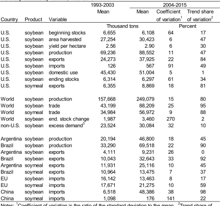
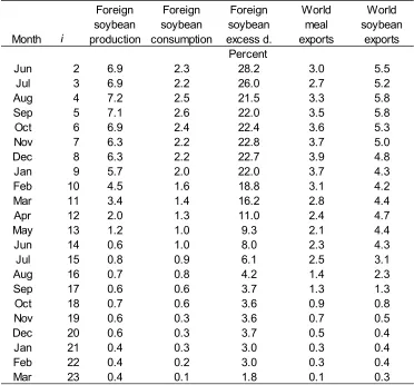
Soybeans has been one of the fastest growing major field crops for several decades, most recently boosted by soaring demand from China. The United States was the world’s leading producer for decades starting in the 1960s, but has been overtaken by South America. World soybean production and consumption is more geographically concentrated than it is for grains or cotton, with the United States, Argentina, and Brazil in 2015/16 accounting for 83 percent of production (89 percent of exports) and China and the European Union (EU) accounting for 75 percent of world imports (Table 1).
The U.S. Department of Agriculture is the source of a broad range of statistics concerning past, present, and future developments in U.S. and world agriculture. USDA has been providing the public with market information since the 1860s in order to improve the efficiency of agricultural markets and reduce
baseline forecasts for the next 10 marketing years. This forecast is updated and published the following February. More prominently, USDA’s monthly reports of U.S. production and world-wide demand and output for grains, oilseeds, and cotton play a crucial role in price discovery on futures markets in the United States and elsewhere. USDA’s National Agricultural Statistics Service (NASS) publishes its Crop Production estimates for the current year for these commodities from August to January, and the World Agricultural Supply and Demand Estimates (WASDE) incorporates these estimates every month, and
extends the forecasts to other balance sheet variables—such as consumption and exports—and also adds geographically dis-aggregated production and consumption forecasts for the entire world. The impact of the information provided by USDA on futures markets has been demonstrated (Fortenbery and Sumner, 1993; Adjemian, 2012; Isengildina, et al. 2008). At least a subset of market participants have a very sophisticated understanding concerning USDA’s estimates, and markets have been shown to anticipate and accommodate to the inefficiencies embedded in USDA’s forecasts (Good and Irwin, 2006,
Isengildina, Irwin, and Good, 2013).
The U.S. demand forecasts and non-U.S. supply and demand the forecasts are the product of committees bringing together expertise from across USDA (Vogel and Bange, 1999). Each Interagency Commodity Estimates Committee (ICEC) is chaired by a member of the World Agricultural Outlook Board (WAOB) and includes representatives from a set of USDA agencies concerned with analyzing and implementing USDA programs.1 The historical data and forecasts developed by a committee consensus are: published
each month in the WASDE, are disseminated through PSD Online, are included in ERS’s Situation and
Outlook reports, are included in FAS’s World Markets and Trade reports, and form the basis of policy deliberations at USDA and other government agencies.
USDA’s Forecasting Cycle
Soybeans are a summer crop, and the U.S. marketing year for soybeans is September-August. Planting in the United States is most active from mid-May to mid-June and harvest during September-October. Planting in the largest producers competing with the United States—Argentina and Brazil—occurs over September-January and harvest there stretches from January to July. Exports from all of these countries are seasonal, with U.S. exports reaching a post-harvest peak during October-February and Southern Hemisphere exports peaking over April-August. Anticipating the length of these peaks is a critical component of USDA’s forecasting task.
The forecasting cycle has four distinct segments, distinguished by the information set available to USDA in each and the Departmental resources devoted to the forecasts. USDA forecasting activity is organized around the U.S. marketing year, with only a few forecasts before U.S. planting and the greatest share of USDA’s resources being devoted to these estimates during the period of U.S. crop development. To compare trade levels on a consistent annual basis, USDA converts the local marketing year data for Brazil and Argentina to an October-September trade year.
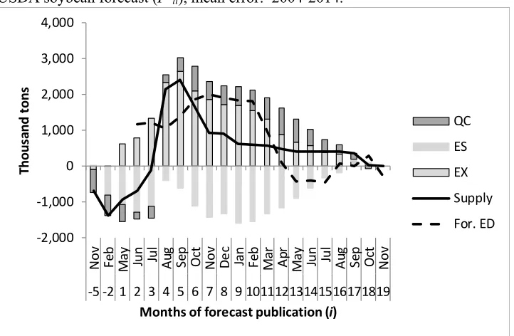
For each marketing year, USDA’s first short-run forecast is developed 10 months before the beginning of that marketing year during preparation of USDA’s long run outlook and of the President’s Budget for the next 5 years (fig. 1). Each November the ICEC develops forecasts for the U.S. balance sheet in the coming marketing year, but this forecast is typically not released until the following February at USDA’s
1Other agencies represented on USDA’s ICECs are: Agricultural Marketing Service (AMS), Economic Research
Agricultural Outlook Forum. This pre-planting forecast is included in the 10 year projections released at the Forum, and an updated forecast for this marketing year is also presented at the Forum. The
information set for these forecasts differs significantly from that for later segments of the forecasting cycle. Many months from finalization, estimates for many variables’ activity in the preceding marketing year are subject to adjustment with observed information. No NASS survey results of U.S. farmers’ spring-sown new-crop acreage intentions are yet available. Dramatic changes in crop prices and climatic conditions can quickly alter farmers’ crop decisions throughout this period. Measuring the forecast horizon (h) of these earliest forecasts as the last month of the marketing year, for November h = 22
months (1.8 years) and for February h = 19 months (1.6 years). These forecasts overlap with forecasts for
the previous marketing year that USDA simultaneously publishes with h = 10 months (November) and for h = 7 months (February). Following the convention used by ICEC members, we term these shorter
horizon forecasts for the previous year as “back-year” forecasts. The distant horizon forecasts are termed “out-year” forecast. This distinction holds through every month of the forecasting cycle that includes forecast for overlapping years, and the forecasts for any given marketing year eventually become back-year forecasts as USDA initiates a forecasting cycle for a new marketing back-year.
Continuous monthly updates of USDA’s forecasts commence in May, and May through July marks another short segment of USDA’s forecasting cycle. During these months, the WASDE includes forecasts
of U.S. production based on the March Prospective Plantings and June Acreage reports from NASS.
Publication of forecasts for the next marketing year in the WASDE start in May and include production
forecasts based on NASS area data and ICEC trend-based yield estimates. Forecasts for the rest of the U.S. balance sheet by the ICEC are also published monthly starting in May as well as for the rest of the world.2 In addition to more accurate estimates of the previous marketing year’s activities, USDA’s ICEC
also has in its information set at this time reports and forecasts from its overseas attaches in the Foreign Agricultural Service (FAS). USDA/FAS maintains offices in China, Argentina, and Brazil—and about 70 other countries—which provide intelligence to Washington-based members of the ICEC, as well as publicly disseminated reports and forecasts. Using information and insights from overseas-based USDA personnel, contacts in industry, public price data, remote-sensing data, meteorological analysis,
contractors for macroeconomic outlook, and a centralized repository of timely international monthly trade data through contractors, USDA maintains historical data and publishes forecasts for the supply and demand for soybeans and other products in over 100 countries. Although the flow of information is constant, the frequency of each source can vary significantly.
August-January marks a more intensive segment of USDA’s forecasting cycle for soybeans and similar crops, as NASS publishes its first estimate of the year’s U.S. crop in August and updates it throughout the harvest period. During these months, forecasts for other aspects of the U.S. balance sheet—and the forecasts for non-U.S. balance sheets—react to changes in the U.S. production forecast and to changes in market conditions around the world. From the beginning of this segment of the forecast cycle, the planting of the U.S. crop is a past event and the issue is no longer forecasting but discovering the actual level of planting activity. Similarly, by the end of this segment yield realization and harvest of the U.S. crop is complete, and the goal of statistical agencies is to reveal this level of past activity.
2May publication of USDA’s non-U.S. soybean forecasts for the coming marketing year has occurred since 2009.
The final segment of the USDA forecasting cycle for U.S. soybeans is February-November. During most of this period, U.S. production is known to within a relatively small margin, while Southern Hemisphere planting levels are discovered and then yield performance in the Southern Hemisphere is also determined. The proportion of the U.S. marketing year’s domestic consumption and export activity that must be forecasted diminishes as monthly reports from the U.S. Bureau of the Census and NASS for past activity accumulate. For example, since 1993, U.S. soybean exports averaged 72 percent complete for the year by March 1, although the range was between 60 percent and 87 percent. Similarly, trade and crush data from industry and government sources in Argentina, Brazil, and elsewhere accumulates as the year progresses, at a rate that varies from year to year.
The finalization of USDA’s estimates for U.S. activity during a given marketing year occurs several months after the marketing year’s conclusion. Ending stocks, trade, and crushing data for the last month of the marketing year (August) is not available before the September WASDE, and NASS typically
finalizes its estimate of the previous year’s U.S. production in October, partly by accounting for information in the stocks and utilization statistics.3 Soybean meal is analyzed on an October-September
year in the United States, so finalization of the U.S. soybean meal estimates occurs one month after the soybean finalization.
A similar process occurs in USDA’s estimates of Brazilian production at the end of the forecasting cycle. While Brazil has respected and timely domestic sources of forecasts and historical estimates of its soybean production, the final estimates from these sources are typically inconsistent with the information in the utilization data. USDA’s October-September estimates for Brazil and Argentina are typically not finalized until several months after the U.S. estimates due to a later ending of their local marketing years and difficulty in reconciling the data from different sources. Soybean stocks data are particularly hard to verify for both countries.
Previous Studies: Inefficiencies in USDA Soybean Forecasts
The importance of USDA’s forecasts to market equilibrium and public and private policy decisions has motivated many studies of USDA forecast performance and a number of studies with a focus on U.S. soybeans. Multi-commodity studies have found inefficiencies in USDA's long run (10-year) forecasts (GAO, 1988 and 1991), but most studies focus on the more widely followed USDA monthly forecasts with a much shorter horizon (h), at most a few months greater than one year (h = 1.3 years). We
summarize these studies first in terms of their findings and then by their methodologies.
Studies of short term USDA livestock forecasts have found inefficiencies in beef, pork (Bailey and Brorsen, 1998; Sanders and Manfredo, 2002), and poultry forecasts (Sanders and Manfredo, 2003). MacDonald (2002) and Isengildina-Massa, MacDonald, and Xie (2012) detected inefficiencies in USDA's cotton forecasts, and other studies have detected inefficiencies in orange, corn, wheat, soybean, and sugar forecasts (Baur and Orezen, 1994; Egelkraut et al., 2003; Botto et al., 2006; Isengildina, Irwin, and Good, 2006; Lewis and Manfredo, 2012). MacDonald examined USDA's trade forecasts (1992, 1999, and 2005) extending the commodities examined to horticultural products as well as livestock and grains, and also finding inefficiencies like bias and serial correlation. A recurring finding across a number of studies and
3Bureau of Census U.S. trade data for the last month of the marketing year was not consistently available for the
commodities is inefficiency in the month-to-month revisions in USDA’s forecasts, primarily
"smoothing," as USDA publishes forecasts whose monthly revisions are often positively correlated with earlier revisions (MacDonald and Isengildina-Massa, 2012a; Isengildina-Massa, Irwin, and Good, 2013).4
Results specific to soybeans have included findings of bias in USDA forecasts of U.S. soybean
production, exports, and ending stocks (USDA, 2004; IKI), and finding the absence of bias in U.S. ending stocks (Xao, Lence, and Hart, 2014—XLH henceforth). Other findings include: forecast smoothing in many parts of the balance sheet (MIM) and forecast smoothing in the production and yield forecasts (IIG). MacDonald (1999) found bias in USDA's oilseed value export forecasts, in contrast with a similar study using earlier data that found no such bias (MacDonald, 1992).
Volatility of the inefficiency measures over time was also found in other studies in addition to the two by MacDonald; that is the measured characteristics of USDA’s soybean forecasts were to some extent determined by the samples examined. Extension of the sample period end point from 1989 in MacDonald (1992) to 1998 in MacDonald (1999) revealed bias. Irwin, Scott, Sanders, Dwight, and Darrel Good (2014) (ISG henceforth) show downward bias in USDA's October soybean production forecasts in 2001-2012 but not in 1990-2000, and IKI show that inclusion of a 2006-2009 dummy in tests of soybean export forecast accuracy indicate downward bias associated with this later period that the authors conclude is not apparent in their overall 1984-2009 sample.
Note that in the 25 past studies of all agricultural commodities reviewed here, the number of years spanned in the historical samples analyzed ranged from 4 (MacDonald, 2005) to 53 (Baur and Orazem, 1994), with a median of 20 years.5
Methodological Similarities Among Past Studies
There are several ways to group past studies by methodology: 1) a clear majority of these studies aim to analyze non-overlapping forecasts, i.e. forecasts with horizons not exceeding the frequency of the forecasted variable, 2) a little more than half of these studies analyzed the forecasts in their published levels form (bushels, acres, ton, etc.), and the rest first applied a transformation into the growth rate forecasts implied by the published data (typically, percent), and 3) a little more than one-third of these studies calculate evaluation measures for aggregated months of the forecasting cycle—presenting a single statistic assessing the entire annual cycle, or an aggregation of a subset of the cycle’s months.
It is necessary to more fully explain the concept of overlapping forecasts before proceeding further. Overlapping forecasts are more complex to evaluate, but—as figure 1 indicates—are unavoidable in studies examining forecasts over the entire USDA forecasting cycle. For example, the cycle’s first forecast for U.S. soybean exports developed in November, 10 months before the start of a given marketing year, includes in its information set a forecast for the preceding marketing year. That preceding-year forecast has a 12 month horizon before the point when USDA can finalize its estimate.
4In the remainder of this paper, several past study references will be abbreviated: Bailey and Brorsen, 1998—BB;
Botto et al., 2006-- BIIG; Egelkraut et al., 2003--EGIG; Isengildina, Irwin, and Good, 2006--IIG; Isengildina-Massa, Karali, and Irwin, 2013—IMKI; Isengildina-Massa, MacDonald, and Xie (2012)--IMMX; MacDonald and
Isengildina-Massa, 2012a—MIM; Sanders and Manfredo, 2002, 2003, and 2008—SM1, SM2, SM3.
5Four studies examined quarterly forecasts, over a median of 15.5 years. In most cases, each quarter’s forecast was
Thus, the first forecast of the cycle is overlapping with a contemporaneous forecast for the previous year, and the same holds true for the following 7 revisions to this forecast spread over the following 12 months, until the previous year’s forecast is finalized.
Some of past studies examined were explicit in selecting to examine only non-overlapping forecasts, selecting a non-overlapping subset of a broader set of a variable’s forecasts. Others studies examined forecasts that were unequivocally non-overlapping, making no reference to the issue. A third group includes studies focused on U.S. production estimates that eliminated overlapping forecasts by
assumption. These studies assign the first January after the U.S. harvest as the point of finalization (BIIG; EGIG; Good and Irwin, 2006; IMIG; IMKI; ISG). Several of these studies examining U.S. production forecasts also evaluate forecasts of other balance sheet variables (BIIG; IMKI; ISG) over a span of the forecasting cycle that includes months with overlapping forecasts. None of these studies, or other studies evaluating forecasts over portions of the forecasting cycle with overlapping forecasts (BB, IMMX, MIM, SM3, and XLH), thoroughly address the impact of overlapping on their evaluation statistics. The impact of overlapping forecasts on the variance-covariance matrix of the evaluation tests is accounted for where appropriate in these studies, but other impacts of overlapping on the evaluation metrics have been overlooked.
Another group of studies are those that examine forecasts as growth rates, in percent, rather than
analyzing them in their published form as a level of activity, e.g. in tons or acres. An appropriate concern addressed by many past studies is accounting for the non-stationarity of the data used in the evaluations (Clements and Hendry, 1998), which is typically addressed by transforming errors from simple
differences to log differences or into percent differences. But the need to correct for spurious correlation is also sometimes addressed by transforming both forecasts and errors into period-to-period differences, or percent growth rates (MacDonald, 1992, 1999, 2002; SM1, SM2; IMMX; IMKI). Other studies motivate such a transformation intuitively (Clough, 1951; Gunnelson, Dobson, and Pamperin, 1972). SM3 use a hybrid approach that decomposes a forecast into a sum of a realized past level added to forecasted increases during subsequent periods.
Aggregation across the forecast cycle is generally undertaken by treating past forecasts as pooled or panel data (e.g. BB, BIIG, IIG, IKI, IMMX, XLH). An advantage of this approach is increased effective sample size, and the disadvantages include homogenizing parameter estimates across potentially different
forecast months and the need to account for correlations between forecast months and years. The expected seasonal similarity among forecast months’ characteristics suggests the loss of month-specific parameters would be acceptable in some contexts, and all the aggregating studies examined here apply strategies to correct their standard error estimates for the interactions between forecasts and for heterogeneous
variances. Correction strategies include using White’s estimator (IMMX, MIM), assuming a constant rate of decline in variance across the forecast cycle (BB, BIIG, XLH), and using the Karali and Thurman (2009) approach of constructing a feasible variance-covariance matrix from OLS residuals (IMKI).
Data
forecast. Over the study period, the countries accounted for 86 percent of global production, 58 percent of global imports, and 89 percent of global exports.
One contribution of this analysis is to drop this restriction and provide the first published analysis of forecasts overlooked in other studies. USDA’s first forecasts from 10 months before the start of the marketing year over 1997-2015 were drawn from USDA’s publications summarizing annual updates to the Department’s long run projections (USDA/OCE, 1998-2016), and the second forecasts disseminated 3 months later at USDA’s Agricultural Outlook Forum were drawn from the grains and oilseeds ICECs’ papers presented at the Forum (USDA/WFGOICEC, 1998-2016). The initial pre-season forecasts presented at USDA’s Outlook Forum over 1993-1996 were not available, but all forecasts published in the WASDE or disseminated with greater international detail elsewhere were collected for these years as
well.
Cornell University’s Mann Library’s comprehensive WASDE archive was the source of USDA’s initial
May WASDE U.S. forecasts over 1993-2009 and its initial June forecasts over 1993-2003; these
publications were also the source of the international marketing year trade forecasts by USDA for Argentina and Brazil over 1993-2002 (USDA/WAOB, 1993-2016). During 1993-2002, USDA’s
Economic Research Service (ERS) disseminated monthly an updated database of USDA’s global supply and demand estimates disaggregated by country, and ERS archives of these releases were drawn upon for this study (USDA/ERS, 1993-2002).6 Since 2002 USDA’s Foreign Agricultural Service (FAS) has
released these updates every month (USDA/FAS, 2002-16) and this study drew on ERS archives of these updates.
The characteristics of these data determined some aspects of our approach to analyzing the forecasts. It was noted earlier that soybean consumption, production, and trade has generally been growing rapidly in recent decades. Therefore, the expected means of these variables vary widely with time, and comparisons across multiple years of forecasts could be skewed by the behavior of forecasts for the years with the highest expected mean. Testing of the 27 variables examined in this study indicated that virtually every series had a mean that varied significantly over the sample studied.7 This motivated our decision to apply
a log transformation to the forecasts, resulting in forecast errors in percent form.
Testing of forecast errors over 1993-2014 revealed the presence of structural breaks in these time series, with a large number of these breaks concentrated around 2002. Sensitivity testing of some characteristics of the forecasts for U.S. production and exports showed some shifts around that time as well as a degree
6In those years, ERS’s database included local marketing year trade forecasts rather than international year forecasts
for these countries, necessitating use of Cornell’s WASDE archives for forecasts of South American trade.
7Data for 27 variables was tested for the presence of unit roots with and without deterministic trends using the
modification to the traditional Dicky-Fuller test developed by Elliot, Rothberg, and Stock (1996). Our concern was not strictly focused on the presence or absence of stationarity, but on variation in expected mean over time for any reason, including non-stationary. The generalized least squares test developed by Elliot, Rothberg, and Stock modifies the augmented Dickey-Fuller test, de-trending the data before testing. In nearly half the variables
of stabilization in years afterwards. Finally, 2004 marked the first year that USDA published its first international soybean forecasts in June rather than July, giving us a forecast cycle with a larger number of forecast months in the 2004-2014 period compared with samples beginning in earlier years. We therefore focused our analysis on USDA’s 2004-2014 forecasts, although we touch on results for longer samples, particularly in the course of sensitivity analysis, and extend the sample to 2015 for the U.S. forecasts.
Finally, the national composition of the EU varied over 1993-2016. Thus USDA replaced its forecasts and historical data of EU soybean trade with those for updated aggregations of countries in 1995, 2004, 2007, and 2013. For the months following each appearance of a new aggregation, we constructed updates to earlier forecasts based on older aggregations based on the average month-to-month revisions to EU totals for the most recent past years published when USDA updated its aggregations.
Forecast Data Notation
We use the following notation for this notation for a given variable’s forecasts:
Fit = USDA’s forecast for marketing year t published in month i.
To increase comparability with previously published forecast evaluation studies, we maintain the
traditional designation of the May pre-season forecast of each year as i = 1, even though it is not USDA’s
first forecast. For the earlier forecasts we then assign negative numbers as labels for the forecast months of November (i = -5) and February (i = -2) that occurred before the end of the previous marketing year (t
-1). These values for i are equivalent to i-12 for overlapping forecasts of marketing year t in November (i
= 7) and February (i =10).
For U.S. soybean variables,
i = -5, -2, 1, 2, … n ; n = 19; t = 1993-2015;
for U.S. soybean meal exports,
i = -5, -2, 1, 2, … n ; n = 20; t = 1993-2015;
and for non-U.S. variables,
i = 3, 4, … n ; n = 24; t = 1993-2003, i = 2, 3, … n ; n = 24; t = 2004-2008, i = 1, 2, … n ; n = 24; t = 2009-2014.
When i = n, the forecast is considered finalized and becomes the variable’s actual realization for that
marketing year:
Fnt = At.
Following transformation into natural logs, we use the convention of lower-case notation:
and first differences (annual change) are indicated using ’:
a’t = at ─ at-1, f ’it = fit ─ at-1, f ’nt = a’t.
Forecast error is the difference of the forecast from actual realized value:
eit = at – fit e’it = a’t – f ’it
To maintain consistency with the majority of past studies, we follow this convention even though it results in a counter-intuitive outcome: when a forecast is larger than the realized value, its error is negative. This convention is consistent with several important theoretic properties of forecasts, resulting in its widespread application (Clements and Hendry, 1998).
The transformation of forecasts into growth rates has been widely applied to address the impact of a variable’s trend on the calculation of important evaluation statistics, but the transformation has further implications for the analysis of overlapping forecasts. To see these implications, first note that when i = j
n-12, forecast error is the same for both the levels forecast ( fjt ) and the change forecast ( f ’jt ) (i.e., ejt = e’jt). But, when i = k < n-12, the error of fkt is the sum of the overlapping errors of f ’kt (the out-year forecast) and f ’k+12, t-1 (the back-year forecast), and ekt ≠ e’kt:
fit = f ’it + a t-1, i n-12
fit = f ’it + f i+12, t-1 i < n-12
fit = f ’it + f ’ i+12, t-1 + at-2 i < n-12
eit = at – fit
eit = (a’t + a t-1) – ( f ’it + a t-1) = a’t – f ’it = e’it i n-12 eit = (a’t + a’ t-1 + a t-2) – ( f ’it + f ’i+12, t-1 + a t-2) = (a’t – f ’it) + (a’t-1 – f ’i+12, t-1) = e’it + e’i+12, t-1 i < n-12 It similarly follows for i < n-12 that,
fi+1,t = f ’i+1,t + f ’ i+13, t-1 + at-2 , so
ri+1,t = fi+1,t ─ fit
ri+1,t = ( f ’i+1,t + f ’ i+13, t-1 + at-2) ─ ( f ’it + f ’ i+12, t-1 + at-2)
ri+1,t = ( f ’i+1,t ─ f ’it) + ( f ’ i+13, t-1 ─ f ’ i+12, t-1)
ri+1,t = r ’i+1,t + r’ i+13, t-1
This study’s primary focus is on f ’it and its associated e’it andr’it. But, we include calculations utilizing eit in appendix tables for some evaluation statistics. Our reasoning is that, even though it is only the change forecasts’ errors (e’it) that give information on USDA’s utilization of information specific to the early forecast cycle (i < n-12), the levels forecasts are what USDA publishes and their errors are the ones more
measurements increases understanding of the forecasting process, and the summed overlapping errors (eit
= e’it + e’i+12, t-1, when i < n-12) may be more important in some contexts and for some readers.
Methodology
We examine each month’s forecasts individually rather than using panel approaches to develop a single characterization across the entire forecast cycle (as in IMKI) or across subsets of months (as in IMMX). USDA publishes 21 versions of a given marketing year’s estimates for each U.S. balance sheet variable, and nearly as many versions of its foreign balance sheet estimates. With about 20 versions of about the same number of variables, more than 400 individual forecasts have to be analyzed if each month in the forecasting cycle is to be considered separately. Despite the resulting large number of forecasts, we retain the identity of each separate month in the forecasting cycle here for two reasons: the considerable
heterogeneity in even some temporally adjacent months, and the applied nature of our analysis.
Conclusions about USDA’s forecasts that address aggregates of forecast months run the risk of being too abstract to contribute to USDA’s efforts to improve the accuracy of its forecasts. The USDA’s forecasters update their forecasts each month, and are keenly aware of the variations in the available information set and analytical resources available in different months. Furthermore, both Isengildina et al (2008) and Adjemian (2012) have highlighted how soybean markets differ from those of other major field crops in responding to WASDE releases outside of the typically crucial window during the U.S. harvest when NASS production forecasts coincide with publication of the WASDE forecasts. It is therefore particularly crucial to maintain a temporally disaggregated approach in evaluating USDA’s soybean forecasts.
MAPE (mean absolute percent error) is the core summary statistic used here to characterize forecast performance.8 We utilize statistical tests to: 1) determine if USDA’s forecasts have increasing or
decreasing accuracy from month-to-month, 2) compare the forecasts in levels to a naïve forecast, 3) test the mean error for its difference from zero (bias), and 4) characterize patterns in USDA’s monthly forecast revisions. Additional analysis examines USDA’s record in forecasting directional change and serial correlation in errors across years. This additional analysis is used to develop deeper understanding of the behavior of selected forecasts. Finally, we also apply a rolling-window search strategy for
sensitivity analysis of the forecast bias tests to distinguish between permanent and evolving
characteristics of the USDA forecasts and to develop hypotheses regarding the sources of forecast bias.
To compare the change in accuracy of USDA’s forecasts from month to month, we apply the Diebold-Mariano test (Diebold and Diebold-Mariano, 2015) to determine in which months USDA’s accuracy improves or diminishes.. As a forecast’s horizon (h) diminishes, the information set available to the forecaster
increases. Thus, the accuracy of forecasts would be inversely proportional to the distance into the future of the events forecasted, and accuracy should improve as that distance diminishes.
The second statistical test is based on the Theil U statistic, which measures the ratio of a forecast’s errors to the ratio of the errors of a random walk, or naïve forecast (Hyndman and Koehlar, 2006). We apply the Diebold-Mariano test to determine the statistical significance of the forecast’s U statistic difference from 1. Forecasts whose accuracy surpasses a random walk’s have U statistic values less than 1 and those underperforming relative to that simple benchmark have U statistic values greater than 1.
8MAPE was chosen for its balanced treatment of unusually large errors. As a measure of central tendency, MAPE is
Bias in the mean of the forecast is the focus of our third test, using the variant of the traditional Mincer-Zarnowitz (1966) test. The more general inefficiency test of Mincer-Mincer-Zarnowitz relied on the regression,
a’t = αi + βi f ’it + εit
which, by assuming β= 1, can be transformed into Holden and Peel’s (1990) variant,
e’it = αi + εit ,
where the test of the significance of the difference of α = from zero becomes the test of forecast bias.
One revision characteristic examined is the relationship between sequential monthly revisions. Nordhaus (1987) introduced an efficiency test that does not rely on the determination of an actual realized value for a forecasted variable, examining the relationship among revisions in the sequence of forecasts addressing a given marketing year. If revisions are designated,
r’it = f ’it – f ’i-1 t
then revisions are inefficient if a non-zero coefficient (φi) describes the relationship between one month’s revision and the revision from the previous month:
r’it = αi + φir’i-1 t + εit
If the forecast is unbiased, then we can assume α = 0, but a biased forecast that met the low efficiency bar of reduced error with reduced distance from the forecast horizon could realize α ≠ 0. Both biased and unbiased forecasts could realize another form of inefficiency where φi ≠ 0. The more intuitive manifestation of such inefficiency occurs when φi > 0, and the forecast is therefore smoothed: new
information in one period is only partly accounted for in that period’s revision and tends to produce a later revision in the same direction. When φi < 0, responses to information in one period are associated with offsetting responses in a following period: rather than smoothed, the forecasts are reverting.9
Bias in revisions is another form of inefficiency, indicative of failure to anticipate predictable patterns of behavior. Biased revisions could be indicative of biased forecasts, since the average direction of revisions in a biased forecast is predetermined, but they are also useful information in their own right. A test for revision bias is whether αi ≠ 0 in,
r’it = αi + εit.
Overlapping forecast analysis introduces another dimension to the characterization of revisions. Testing for the significance of the correlation (ρ) between the simultaneous month-to-month revisions of different marketing years’ forecasts for a given variable does not necessarily test for an inefficiency, but can be useful information about forecasters’ utilization of information. Sample correlation in this case is calculated as:
ρ = Σ , , * Σ ∗ Σ , ,
/
To guard against the influence of outlying observations we take the precaution of only testing for the significance of the difference of ρ from zero when the null hypothesis of normality in the Shapiro-Wilk test cannot be rejected for both r’it and r’i+12 t-1.
Evaluation of directional accuracy for fit based on 2x2 contingency tables provides additional insight into forecast behavior, an approach with roots going back as far as Zarnowitz (1967). Using χ-squared tests with large samples and Fisher’s exact test in studies like this one, the test determines the probability that a forecaster’s share of directionally accurate predictions is independent of observed events, and therefore has value (Joutz and Stekler, 2000). In some instances in this study, the test could not be applied because either every year’s actual realization is in the same direction—as in China’s soybean imports—or the USDA’s forecast was in the same direction every year—as in forecasts for Argentine meal exports until i
= 10. Further, a preponderance of actual changes in one direction creates a high bar for USDA to demonstrate independence, with a greater than 90 percent directional accuracy share needed to reach or surpass 5 percent significance in the forecasts for several variables. To avoid these issues, we apply Fisher’s exact test on contingency tables for forecasts of the direction of change in the annual changes forecasted ( f ’it) to gain some insight into USDA’s forecasts of some variables.
Results
We first provide an overall summary of the results, and then give more detail for each evaluation
measure. We used a subset of the variables’ forecasts examined in this study to create summary statistics for each evaluation measure, for each month of the forecast cycle. The subset excluded U.S. area and yield, and excluded the geographically aggregated variables—such as world trade or foreign production— and the summary statistics are only calculated for forecast months when non-U.S. variables were forecast during 2004-15, i.e. no earlier than the first June of the forecast cycle, i = 2.
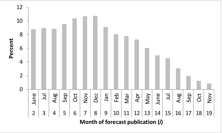
The median MAPE of our subset of forecasts ranges between 8.8 percent and 7.7 percent between June (i
= 2) and the following March (i = 10), and begins falling relatively steadily after December (i = 8) (fig.
2). The first forecast month with median MAPE that is less than or equal to half the level of i = 2 is the
second August (i = 16). Among the variables forecast, MAPE is generally greatest for variables with
relatively low levels of activity. Residually forecast variables—like U.S. ending stocks and foreign excess demand also have relatively high MAPE.
Theil U statistics reveal relatively few problems, with only 7 out of all of the forecasts examined ever realizing a U > 1 in any month. There are only 6 examples of variables whose USDA forecasts in any month are significantly less accurate than a naïve forecast and a maximum of two such variables—or 12 percent of the forecasts—in any given month (fig.3). Months i = 4 and i = 5 are the worst for USDA with
respect to evaluation using the Theil U statistic, and i = 6 is the last month when any USDA forecast is
significantly less accurate than a naïve forecast.
In the Diebold-Mariano testing of the monthly changes in MAPE, month i = 4 stands out as a forecast
Bias is the most broadly realized inefficiency found in this set of USDA soybean forecasts. At 47 percent, its share of affected forecasts (in month i = 10) is tied with smoothing as the highest of any
statistical test in any month. The last month any member of our subset realizes significant bias is i = 18,
but some aggregated variables are biased to the very end of the forecast cycle. In the detailed results by evaluation measure below and in the subsequent discussions, bias receives the most attention.
Smoothing is also broadly realized, but is less prevalent in the forecasts examined here than is bias. While the i = 13 peak of 47 percent of our subset of forecasts realizing smoothing matches the peak
month for bias, the prevalence of smoothing tends to be lower than bias in virtually any other month of the forecast cycle.
Mean Absolute Percent Error (MAPE)
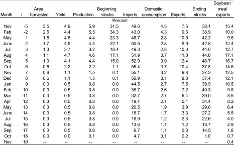
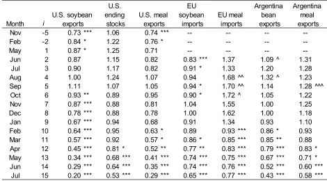
Two immediate observations about USDA’s forecasts ( f ’it) are derived by comparing the more general statistical characteristics of the forecasted variables (Table 1) with their 2004-2014 MAPE (Tables 2, 3 and 4). 10 One is the association of higher variability/trend-share ratios with larger errors, such as with
U.S. ending stocks. Another is that trade variables’ forecasts generally have higher MAPE than
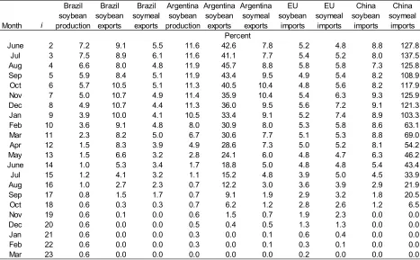
production variables’, but that a trade variable’s MAPE is generally inversely proportional to the volume of trade. Among the trade variables forecast, U.S. soybean imports and China’s soybean meal import forecasts have the highest MAPE (peaking at 50 and 128 percent respectively), and the lowest annual volume, less than 1 million tons annually over 2004-2014. Similarly, Argentina soybean exports MAPE surpassed 40 percent in some months—comparable to U.S. soybean ending stocks—but these exports averaged under 10 million tons over 2004-2014. U.S. and Brazil soybean export MAPE never exceeds 13 percent, and volume averaged 30-40 million tons. Note that forecasts of some variables representing highly aggregated data—such as total world trade—have very small MAPEs (2-5 percent) thanks to offsetting errors among their components (Table 4).
Early-cycle U.S. beginning stock forecasts have MAPE levels that exceed those of most other balance sheet variables even after the completion of the previous marketing year. Beginning stocks out-year forecasts for year t in i = 5 (September, f ’5t) are equivalent to back-year ending stocks estimates for the previous year (t-1) in their 16th month of revision (i = 17, f ’17,t-1). This means that even though the previous marketing year’s errors specific other balance sheet variables have been filtered out by
converting the levels forecasts to change forecasts, back-year errors still find their way into the out-year estimates through beginning stocks.
Comparing out-year beginning stocks’ annual-change forecasts ( f ’it) MAPE with the MAPE for levels forecast of stocks ( fit, Appendix table 1) shows they are virtually equivalent, appropriately, since the previous year beginning stocks forecasts ( f ’i+12,t -1) have virtually no error.11 Most other variables have higher MAPE for forecasts of levels, but the exceptions—e.g., Argentine soybean exports, U.S. ending stocks—are instructive. MAPE is only smaller for the out-year change forecast when the overlapping forecasts have a common directional error and correlation. Negative correlation of overlapping errors is
10See Appendix tables 1, 2 and 3 for the MAPEs of the levels forecasts (fit).
11 The past-year change error (e’i+12,t-1) included in the forecasts evaluated in the Appendix Tables ( fit) is from a
an important factor in explaining how the MAPE of a sum of overlapping errors (eit = e’it + e’i+12, t-1) can be smaller than the MAPE of one component of that sum (e’it).
Test of Theil U Statistics
The patterns observed in testing the fit Theil U statistics suggested that only a subset of forecast’s results warranted detailed discussion. For example, all three production forecasts examined had U statistics significantly below 1 in every month of the forecast cycle, as did every forecast of China’s imports; this is consistent with the large role that previous-year prices play in determining the level of production and the fact that China’s imports rose every year in the 2004-2014 sample.12 Table 5 is restricted to only the
forecasts with U statistics that exceeded 1 in any month.13 As was the case with MAPE, the Theil U
results for U.S. soybean ending stocks indicate this variable’s forecasts have the weakest performance of any balance sheet variable. USDA’s forecasts fail to prove statistically superior to a random walk until April (i =12). Earlier in the cycle (i = 4), the U ratio rises to nearly 30 percent above 1, but the variability
that makes forecasting this variable so difficult also prevents the superiority of the naïve forecast from reaching statistical significance.
The European Union (EU) soybean meal forecasts mirror the U.S. ending stock forecasts in that their Theil U rises from a little more than 1 at the start of the forecast cycle to about 1.3 during i = 4-6. An
important difference for the EU variable is that the naïve forecast is statistically superior to USDA’s. USDA’s forecasts for EU beans and meal imports don’t achieve statistical superiority over the naïve forecast until February and March (i = 10 and i = 11). Table 1 shows that the ratio of variability to trend is
relatively low for EU meal imports, and MAPE—at little more than 6 percent—is relatively low as that ratio often indicates, but compared with the naïve forecast benchmark, this is one of the most poorly performing forecasts.
Southern Hemisphere exports also show some months when USDA significantly under-performs relative to the naïve forecast. Argentine soybean and meal exports in months i = 4 and i =5 are examples of this
and will be examined again when reviewing the Diebold-Mariano testing of the month-to-month changes in USDA’s MAPE.
Monthly Patterns of Changing MAPE
Using the Diebold-Mariano test with a mean absolute error loss factor to compare 2004-2014 forecasts in logs from one month of the forecast cycle ( f ’it) with the same years’ forecasts published in the preceding month ( f ’i-1t) allows us to determine if the observed monthly change in MAPE is statistically significant. We observe that most latter months of the forecasting cycle are characterized by consecutive significant increases in accuracy (Tables 6 and 7), and also that accuracy declines in some months, particularly early in the forecast cycle. The longest continuous strings of consecutive monthly improvements in accuracy are 10 months (Argentina’s production) and 9 months (U.S. soybean exports and China soybean imports). Early-cycle August (i = 4) stands out as the month with the most variables’ forecasts realizing negative
12Note that Brazil’s 2004 production level was significantly affected by drought. Using the standard 2004-2014
sample USDA’s forecast was not superior to a random walk until well into the marketing year. Dropping the outlying year resulted in a sample believed to be more representative of likely future behavior.
13Appendix table 4 has the U statistics for the entire U.S. balance sheet. The remaining calculations are available
accuracy shocks. A total of 7 variables’ forecasts experience significant MAPE increases in August, compared with a total of 4 forecasts in July, and 3 such forecasts over the 3 months following August.
Earlier, we noted USDA’s U.S. ending stocks forecasts had high early-cycle MAPE and failed to
significantly surpass the naïve forecasts until late in the cycle. Diebold-Mariano testing shows the absence of month-to-month improvement in the ending stocks forecasts until i = 12 (April). The ending stocks
forecasts also stand out for a one-month decline in MAPE of 14 percentage points at virtually the end of the forecast cycle, i = 18. This one month improvement in accuracy exceeds even the largest MAPE ever
realized by several other variables at any point in the forecasting cycle. This highlights both the large initial magnitude of the errors in the ending stocks and the extent to which convergence to the actual realization tends to be postponed. A 2.5 percent mid-cycle deterioration in accuracy (January, i = 9) for
the U.S. ending stocks forecast also stands out: note that every other U.S. balance sheet variable significantly improved in that month during 2004-15, suggesting U.S. ending stocks are forecast as a residual. Accuracy deteriorates for some variables a little later than this, such as in U.S. domestic consumption and China’s imports, but these don’t exceed 0.2 percentage point increases in error.
A standout for early-season poor performance is the forecast for EU soybean meal imports, which experienced declining month-to-month accuracy in 5 out of 6 months from July to December. EU meal imports and U.S. meal exports were the only variables to experience 3 consecutive months of
significantly increasing MAPE; U.S. soybean exports and consumption each experienced 2 such consecutive months, concluding in i = 5 (September).
U.S. production forecasts in 2004-2015 experienced a 1.4 percent increase in MAPE in August (i = 4), a
development that seems counter-intuitive since by the beginning of August a number of the factors influencing U.S. yields have run their course and are no longer subject to error-prone forecasting. The statistically significant declines in MAPE realized through July (i = 3) are indicative of this process. No
significant improvement occurs in September, but a 2.2 percentage point decline in MAPE is realized in October, with further improvements in November and January. Notable as well is that non-trivial improvement occurs at the end of the forecasting cycle, 0.8 percent points in October and an additional small, but statistically significant, improvement of 0.1 percentage points in November. Recall that most forecast evaluations of U.S, production assume January (i = 9) marks the point of realization. Interactions
between balance sheet components were not the focus of most of these studies, which were focused exclusively on production or yields. But exploring the sources of later-cycle errors in USDA forecasts of ending stocks and exports must consider the errors implicit in multi-million ton revisions in USDA’s production estimates at the end of the forecast cycle. Marking January (i = 9) as the end point of the
forecasting cycle is akin to discarding important information about USDA’s soybean forecasts.
Comparing the Diebold-Mariano tests on the forecasts in levels form (Appendix tables 5 and 6) highlights a few characteristics of USDA’s forecasts. The levels forecasts ( fit) of U.S. soybean meal have accuracy deteriorating less in June (i = 2) than the change forecasts ( f ’it) do—and improve slightly in July (i = 3) while the change forecasts again deteriorate—because improvement in the previous year’s forecasts ( f ’
i+12, t-1 ) offsets some of the out-year deterioration. Similarly, the EU soybean meal import forecasts are
relatively unremarkable in their early-season accuracy deterioration when tested in levels form than when tested in change form for the same reason. USDA’s July (i = 3) forecast for Brazilian soybean production
was unchanged in levels from June in every year of the 2005-14 sample examined there, whereas the implied change forecast deteriorated in accuracy (slightly), reflecting the month i = 15 change in the
Bias in Forecast Means
At least one variable’s forecast in the U.S. soybean balance sheet was biased in every month over 2004-15, but bias in multiple variables’ forecasts was more common, often as many as 4 at one time (Table 8). U.S. trade variables are the most consistently biased, sustaining runs of consecutively biased months of 11 months (exports), 12 months (imports), and 13 months (meal exports). Bias in USDA’s forecasts of EU soybean meal imports was found for 16 consecutive months, but other-wise, non-U.S. variables realized much shorter stretches of sustained significant bias through the forecasting cycle. Sensitivity testing indicates sustained upward bias in U.S. ending stock forecasts since the early 1990s, and downward bias in the U.S. soybean export forecasts that has grown in magnitude and spread to
increasingly early portions of the forecast cycle in the most recent rolling-window samples. Shifts in signs and magnitude of bias in USDA’s forecasts of U.S. production and foreign excess supply coincided with the changes in bias in the U.S. export forecasts.
In the first months of USDA’s forecasting cycle during 2004-15, bias was virtually absent from the U.S. soybean balance sheet forecasts, confined exclusively to beginning stocks in November (i = -5) and then
to imports in February (i = -2). Mean error is relatively close to zero in these initial months for ending
stocks, soybean exports, and soybean meal exports, but rises in absolute terms and becomes significantly different from zero in a few months. Production mean error begins rising in month i = 3 but only becomes
significantly different from zero in month i = 4, and then becomes consistently unbiased in this sample.
Domestic use’s bias is confined to month i = 18. Note that the bias in soybean export forecasts also
persists until i = 18, the last of 11 consecutive months of downwardly biased forecasts.
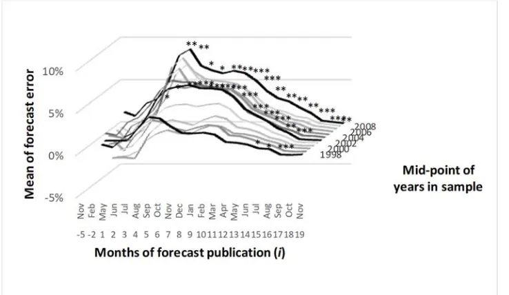
Sensitivity testing through rolling-window estimation of 12-year samples over 1993-2015 shows how bias in USDA U.S. soybean ending stock forecasts has persisted over decades in some months of the forecast cycle, and diminished in others (fig. 4). In the most recent sample period, 2004-2015, only one month before month i = 6 had an average error different from zero with at least 10 percent significance. Earlier,
in the 1997-2008 sample (centered in 2002), significant bias was observed in three early months, and in the oldest sample, bias was observed continuously from i = 1 to i = 11.14
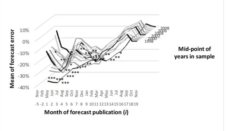
Applying the same rolling-window analysis of mean forecast error to 12-year samples of mean errors in the U.S. production forecasts shows that the 2004-2015 bias shown in Table 8 is a recent phenomenon (fig. 5). Confining our discussion to the same 3 representative samples used for ending stocks, we see significant differences from zero for only a few months, and only in the most recent sample. A few 12-year samples outside these 3 showed small negative bias in the late months of the cycle, but none of the large positive mean errors in the early-cycle months of the oldest sample were significantly different from zero in statistical testing.
The last U.S. balance sheet variable’s bias estimates we subject to sensitivity testing are those for soybean exports (fig.6). Over 1993-2015, bias was always present late in the forecast cycle, but in the oldest samples bias was absent from the forecasts of the earlier months. The sample with the largest and most extensive bias was the most recent one, 2004-2015. Comparison between figures 5 and 6 is suggestive of a link between the peak bias periods months of i = 4 and i = 5 in both the production and export forecasts,
14Samples for intermediate periods showed bias with magnitude and degree of persistence essentially consistent with
but fully understanding the intra-seasonal and year-to-year variation of USDA’s U.S. soybean export forecast bias requires still further examination. In the Discussion section of this paper, we address this issue further.15
Bias and USDA’s non-U.S. Forecasts
Most of the non-U.S. variables analyzed had significant bias in more than one month of the forecast cycle (Table 9).16 The greatest mean error difference from zero was observed in foreign excess demand (7.6
percent, i = 10), but this difference was not statistically significant. The largest significant mean errors
occur in i = 9, for EU soybean meal imports (-6.8 percent) and Argentina soybean meal exports (-6.2
percent). The 16 months of consecutive bias for 2004-15 forecasts of EU soybean meal imports was mentioned earlier. The next longest run of consecutively biased months for any variable is for foreign soybean production during the last 9 months of the forecasting cycle. Both world trade and China’s imports are downwardly biased for 6 consecutive months near the end of the forecasting cycle. In addition, foreign soybean production and consumption are biased downward during 2 of those months.
Sensitivity testing finds that upward bias in the EU and Argentina meal trade is a recent phenomenon, found only in the most recent samples and reversed in the very oldest samples. In contrast, forecasts of China’s soybean imports have been downwardly biased for decades, with the bias much larger in the oldest samples. But, in the 1990s when bias sometimes surpassed 30 percent, China’s role in world markets (prior to its WTO accession) was negligible. More recently, while China’s bias is much smaller in proportional terms, China has come to dominate both world trade and U.S. soybean exports. Since 2008/09, China has imported more U.S. soybeans than all remaining U.S. trade partners combined, so biased expectations regarding China’s imports has significant implications for forecasting U.S. exports.
Sensitivity testing of the mean error in foreign excess demand shows trends that likely reflect this growing role of China’s influence on USDA’s global soybean forecasts. Figure 7 shows the 1993-2014 mean error in rolling samples of a simulated measure of forecasted foreign excess demand. Note that while Table 9 shows excess demand errors averaging as much as 7.6 percent, figure 7 shows that the difference between USDA’s foreign consumption growth forecasts and its foreign production growth forecasts never exceeds 1.7 percent, but is statistically different from zero. Both estimates are consistent with mean errors for foreign excess demand in month i = 10 over 2004-2015 of 2-3 million tons, which
was also the range of the mean error in USDA’s U.S. soybean export forecasts over 2004-14 in the middle of the forecast cycle.
Bias and Overlapping Forecasts
15 Using the definition of domestic consumption used in the WASDE’s world balance sheets, we don’t observe
similar patterns in bias for USDA’s forecasts of U.S. domestic consumption. However, if we remove “residual” consumption from total consumption—leaving the sum of crush and seed use—we observe a number of late-cycle months with downward bias in the 2004-15 sample and a trend over time of an increasing number of months realizing bias.
16 Of the global variables analyzed, a smaller share was biased than was so for the U.S. variables. Less than half of
A common pattern emerges when comparing a variable’s mean error of forecasts in levels ( ) with its mean errors of forecasts of annual change ( ): the absolute value of the levels forecast errors (Appendix tables 7 and 8) are almost invariably at their largest at the beginning of the forecast cycle, but the change forecasts begin the cycle with smaller absolute mean errors. These mean errors ( ) then rise for several months before beginning to diminish. Even the variables whose levels forecasts ( fit) have the largest mean errors in absolute value terms have much smaller—and statistically insignificant—absolute values for their mean forecast errors in the first few months of the forecast cycle for their change forecasts ( f ’it).
The relationship between the pair of overlapping change forecasts of a variable and its out-year levels forecast is more apparent with forecast bias than it is for most forecast evaluation statistics. Bias in the out-year level forecast in sample years t to T is the sum of bias in the out-year change forecast over t to T
and the bias in the back-year change forecast over t-1 to T-1. Comparison of U.S. soybean import forecast
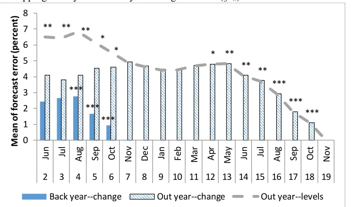
mean error in Table 8 and Appendix Table 7 is illustrative: = 31 percent, = 44 percent, and = 74 percent, approximately the sum of the first two.17 A graphical comparison for China soybean import
forecast mean error illustrates the point across several months of the forecast cycle (fig. 8). For the out-year, the levels forecast is significantly (10 percent significance level) biased during the first 5 months of the cycle, whereas the out-year change forecast is not significantly biased until nearly a year after the first estimate. The back-year estimate is biased in months i = 4 to i = 6, corresponding to the significant bias
for the out-year forecast in months i = 16-18.
Analysis of Forecast Revisions
Forecast revision behavior by USDA was examined 3 ways: measuring the relationships between sequential monthly revisions of forecasts for the same marketing year (smoothing or reversion), testing the mean of forecast revisions in a given month of the forecast cycle over the sample period (bias), and measuring the correlations between the simultaneous revisions of forecasts for marketing years t and t-1
in a given month.
Only one forecast showed a pattern of sustained smoothing or reversion throughout the forecast cycle, late-cycle forecasts for U.S. soybean exports. For the overall group of forecasts, testing showed only 7 of the 20 examined had at least 2 sequential months in the forecast cycle with either significant smoothing (φi > 0) or reversion (φi < 0). Other than the 7 forecasts included in Table 10, only one other forecast had more than 2 months of even non-sequential smoothing or reversion.18 U.S. domestic consumption and EU
soybean imports were the only variables whose forecasts ever tested for significant reversion in any month, and in each case the result was driven by an outlying observation, a problem highlighted in MacDonald and Isengildina-Massa (2012b).
The second December of the forecast cycle (i = 8) marks the beginning of a period when smoothing was
at its most widespread in the 2004-15 sample. Two or more variables tested for smoothing every month from months i = 8 to i = 14. March (i = 11) and May (i = 13) were peak months in this respect, with 5 and
6 forecasts realizing smoothing respectively. U.S. soybean export forecasts were the most consistently
17Recall that
7
′ has a sample of 2004-2015, while the comparable back year average embedded in 5
′ has
a sample of 2003-2014. Using the correct samples, ′5 + 7 ′ =
5
′ exactly.
18Forecasts of Brazilian soybean exports were smoothed in August (i = 4), December (i = 8), and in the following
August (i = 16).
smoothed, with 7 consecutively smoothed months (i = 9-15), and a total of 9 such months over the entire
forecast cycle. No other variable had more than 2 consecutive months of smoothing in this study. U.S. ending stocks was the variable with the next greatest number of smoothed months, 5 in total. Note that forecasts of production of soybeans in the United States were not smoothed in our findings, using a 5 percent threshold. USDA’s November (i = 7) forecasts came quite close, with a smoothing coefficient of
0.028 with a significance level of 5.2 percent.
In the tests for revision bias, the U.S. soybean export forecasts again stand out, with average revisions significantly different from zero in 6 out of the 8 last months of the forecasting cycle (Table 11). U.S. soybean exports’ revision bias is confined to the end of the forecast cycle, and is always upwards, whereas U.S. soybean meal export forecasts had both downwardly-biased early-cycle revisions and upwardly-biased revisions afterwards. Forecasts for China’s soybean imports were similar to the U.S. soybean export forecasts in the respect that they had upwardly biased revisions in 2 out of the last 3 months of the forecast cycle. The biggest downwardly biased revision in U.S. soybean meal forecasts coincides with a downwardly biased revision in production, in month i = 4. Both forecasts have
downwardly biased revisions in month i = 2, but the production bias in that month is extremely small.
Few of the variables studied here had one or more months with biased revisions, and the median number of variables with biased revisions in any given month over i = 3 to i = 21 is 1. Therefore, we do not
include comprehensive tables for all variables of this statistic, including only a subset of the U.S. results in Table 11, along with their associated overlapping forecast revision correlations.19 The months with
exceptional numbers of variables with biased revisions are i = 2 (with 6 such variables), i = 4 (5
variables), and i = 19 (4 variables). Note that an overwhelming majority of the instances of revision bias
are associated with U.S. variables, including all such instances in i = 2.
In contrast with revision bias, instances of significant correlation between revisions to overlapping forecasts are more common in the non-U.S. forecasts (Table 12) than in those for U.S. soybean variables. For both U.S. and non-U.S. variables, such correlations are exclusively negative, even though negative annual serial correlation in the actual year-to-year changes is not a characteristic of any of the variables studied here. Since neither is positive serial correlation statistically significant in the actual year-to-year changes for any variable (other than EU soybean imports), it is not immediately obvious that this
characteristic is an inefficiency. However, we can observe instances when the characteristic is associated with an increase in absolute mean error as the forecast cycle progresses. We can observe that the largest monthly deterioration in the accuracy of China’s soybean import forecasts in the forecast cycle occurs in i
= 7, and that month’s revision is correlated with the overlapping forecast revision in i = 19, which is a
biased revision. The i = 7 revision is not biased, but is unhelpful, the last in a string of increases in the
absolute value of the mean 2004-14 error that began 3 months earlier. The absolute value of the variable’s mean error peaks in month i = 7, and begins testing as bias 6 months later. Similarly, Argentine meal
exports’ revisions are negatively correlated with overlapping forecast revisions in every consecutive month from i = 3 to i = 6, a period of steadily rising absolute mean error to its peak. Mean error becomes
statistically different from zero 3 months later.
19Revision bias instances excluded are U.S. beginning stocks in i = 2 (-5.5 percent) and i = 5 (-4.0 percent); U.S.
Negative correlation of overlapping revisions of change forecasts is in one sense a function of rational forecasting strategy for levels forecasts. A rational appraisal of the information set available for early-cycle foreign variable forecasts leads to a small number of revisions in the months immediately following publication of USDA’s first out-year forecasts for these variables. At the same time, overlapping back-year forecast revisions are inevitable, and with out-back-year, early-cycle levels forecasts relatively fixed, negative correlation in the change forecasts is inevitable. Recall that,
ri+1,t = r’i+1,t + r’ i+13, t-1,
so, if ri+1,t = 0, then
r’i+1,t = ─ r’ i+13, t-1,
and a tendency to not revise fit results in the observed pattern. Since early-cycle U.S. variable forecasts in levels are typically revised about as much as late-cycle forecasts, we observe less of this negative
correlation in the overlapping forecast revisions for U.S. variables.
Directional Accuracy
In general, USDA’s production forecasts’ directional accuracy is distinguishable from a random outcome earlier in the forecast cycle than it is for other components of the balance sheet (Table 13), consistent with the earlier physical realization of the event being forecast. An exception here is Brazilian production forecasts, which have one of the latest realizations of consistent non-randomly correct forecasts, i = 21.
This is in part a function of the largely uni-directional nature of annual change in this variable (rising in 82 percent of the sample years), but also likely indicative of systemic issues in USDA’s Brazil soybean production forecasts, as evidenced by the mid-cycle downward bias.
Other problematic forecasts see similarly delayed realization of consistent, statistically significant directional forecast accuracy for USDA: EU soybean meal imports (i = 20) and U.S. soybean meal
exports (the longest delayed U.S. forecast, with i = 16).
Discussion
Evaluation can reveal forecasts with high error and/or significant inefficiencies, and a logical next step is thinking about measures to improve forecasts. But there is an implied intermediate step: understanding the sources of forecast error. Understanding the source of errors requires understanding the sources of the forecasts, which can be collected into three groups: the causes of the actual events forecasted, the
information set available about these events, and the interpretation of the information set to produce the forecast.
Focusing on the interaction between bias in the U.S. ending stock and export forecasts, we will develop a description of how the underlying physical processes of world soybean markets and USDA’s