A Fast Fourth Order Method for 3D Helmholtz Equation with Neumann Boundary

(1)

ISSN Online: 2161-1211 ISSN Print: 2161-1203

DOI: 10.4236/ajcm.2018.83018 Sep. 12, 2018 222 American Journal of Computational Mathematics

A Fast Fourth-Order Method for 3D Helmholtz

Equation with Neumann Boundary

Na Zhu, Meiling Zhao

School of Mathematics and Physics, North China Electric Power University Department Name of Organization, Baoding, China

Abstract

We present fast fourth-order finite difference scheme for 3D Helmholtz equ-ation with Neumann boundary condition. We employ the discrete Fourier transform operator and divide the problem into some independent subprob-lems. By means of the Gaussian elimination in the vertical direction, the problem is reduced into a small system on the top layer of the domain. The procedure for solving the numerical solutions is accelerated by the sparsity of Fourier operator under the space complexity of _{O M}

( )

3 _{. Furthermore, the} method makes it possible to solve the 3D Helmholtz equation with large grid number. The accuracy and efficiency of the method are validated by two test examples which have exact solutions.

Keywords

Helmholtz Equation, Fourier Transform, Neumann Boundary Condition

1. Introduction

Helmholtz equation appears from general conservation laws of physics and can be interpreted as wave equations. Helmholtz equation is widely applied in the scientific and engineering design problem. Many methods have been proposed for solving the Helmholtz equations, such as finite difference method [1], finite element method [2] [3] [4], spectral method [5] [6] and other methods [7] [8] [9]. However, the computational cost of the finite element method increases greatly for large wave number problems. Additionally, boundary element me-thod is limited to constant-coefficients problems. Finite difference schemes pro-vide the simplest and least expensive avenue for achieving high-order accuracy. Some high order algorithms are proposed in [10] [11] [12] [13]. In this paper, we derive a fourth-order finite difference scheme using 19 points for solving the

How to cite this paper: Zhu, N. and Zhao, M.L. (2018) A Fast Fourth-Order Method for 3D Helmholtz Equation with Neumann Boundary. American Journal of Computa-tional Mathematics, 8, 222-232.

https://doi.org/10.4236/ajcm.2018.83018

Received: July 28, 2018 Accepted: September 9, 2018 Published: September 12, 2018

http://creativecommons.org/licenses/by/4.0/

(2)

DOI: 10.4236/ajcm.2018.83018 223 American Journal of Computational Mathematics

three-dimensional Helmholtz equation.

The discretization of the fully three-dimensional Helmholtz equation contains a large number of unknowns and requires considerable memory space. The time and space complexity increase exponentially as the grid number increases. In the meantime, to maintain a given accuracy, the mesh must be refined as the wave number increases. Some parallel algorithms are presented in [14] [15]. However, this kind of parallel algorithms cannot settle the conflict between the grid num-ber and the performance of the computer hardware.

Fast Fourier transform is a powerful technique for solving the Helmholtz equ-ation both in two and three dimensions [16] [17]. However, fast algorithm in [18]

requires much computational cost. In light of this, we propose a fast algorithm for solving the three-dimensional Helmholtz equation. The fast operator applies inexpensive transformation to break the large discretization matrix into small and independent systems. Therefore, the equation in the whole region is divided into some small equations in the vertical direction. Meanwhile, the algorithm saves much memory space and requires less computational time due to the spar-sity of the fast operator. The problem is reduced on the aperture by introducing a Gaussian elimination and the Neumann boundary condition in the vertical di-rection.

The paper is outlined as follows. In Section 2, a fourth-order finite difference method for the Helmholtz equation is derived. In Section 3 and Section 4, a fast algorithm is proposed by the Fourier transformation and Gaussian elimination. Two numerical experiments of the fast fourth-order algorithm are presented in Section 5. The paper is concluded in Section 6.

2. Fourth-Order Finite Difference Method

The model problem is described as follows

(

)

2 _{, in}

, , , on \

f b x y z

k

φ φ

φ

= Ω

= ∆

∂Ω +

Γ

(1) in the cubic domain Ω_{with Neumann boundary condition}

( )

, , on ,

g x y n

φ

∂ ₌ _Γ

∂ (2)

where k is the wave number and Γ _{is one of the planes of domain.}

(

, , ,

) (

, ,

)

f x y z b x y z and g x y

(

,

)

are known function. The Helmholtz equa-tion is approximated by a fourth-order finite difference discretizaequa-tion with

h= ∆ = ∆ = ∆x y z and the partition

{

(

x y zi, ,j l

)

}

_{i j l}M_{, , 0}1,N1, 1L

+ + +

= .

The 19-points finite difference stencil with h yields the following linear system

(

)

(

)

(

)

( )

2 2 2

2 2 2 2 2 2 2 2 2 2

, , , , , ,

2

2 2 2 2 2 2 4

, , , ,

1

12 6

12

x y z i j l x y x z y z i j l i j l

i j l x y x z y z i j l

k h h _k

h

f f O h

δ δ δ φ δ δ δ δ δ δ φ φ

δ δ δ δ δ δ

 

+ + + + + + +

 

 

+ + + +

= ，

(3)

where 2_, 2

x y

δ δ

and 2

z

(3)

and

φ

i j l, , is the fourth-order finite difference solution of Equation (1). Moreover, we can write Equation (3) in the matrix form

(

)

(

)

(

)

2 2 2 2 2 1 12 6 , 12

M N L M N L M N L

M N L M N L M N L B

k h _A _I _I _I _A _I _I _I _A

h A A I I A A A I A k

h

F A I I I A I I I A F F

 

+ ⊗ ⊗ + ⊗ ⊗ + ⊗ ⊗ Φ

 

 

+ ⊗ ⊗ + ⊗ ⊗ + ⊗ ⊗ Φ + Φ + Φ

= + ⊗ ⊗ + ⊗ ⊗ + ⊗ ⊗ + (4) where

(

)

(

)

(

)

(

)

(

)

2 2 2

T

1,1,1 1,1, 1,2,1 1,2, 1, , , ,

T

1,1,1 1,1, 1,2,1 1,2, 1, , , ,

1 _{tridiag 1, 2,1 ,} 1 _{tridiag 1, 2,1 ,} 1 _{tridiag 1, 2,1 ,}

, , , , , , , , , , , , , , , , , , , ,

M N L

L L N L M N L

A A A

h h h

F f f f f f f

φ φ φ φ φ φ

= − = − = −

Φ =

=

   

the symbol ⊗ represents the Kronecker product. I I IM, ,N L and IMNL are

identity matrices, the subscripts denote their dimension. A AM, N and AL are

,

M M N N× × _and L L× _{tridiagonal matrices respectively.}Φ_B_and F_B are the boundary parts of Φ_and_F_.

3. Fast Algorithm for Three-Dimensional Helmholtz Equation

M

A and AN are all tridiagonal Toeplitz matrices. Fourier-sine transformation

can be applied to these matrices for accelerating the algorithm. Multiplying dis-crete Fourier-sine transformation matrices SM and SN on the both side of

M

A and AN, we have

(

)

(

)

1 1 2 2 1 2

Λ diag , , , , Λ diag , , ,

M M M M N N N N

S A S = = λ λ _ λ S A S = = µ µ _ µ _,

where

( )

(

)

2 2

₍

₎

,

4 1

2 _sin π _, _sin π _{,1 ,} _.

1 1 2 1

M i j i

M

ij i

S i j M

M M λ a M

+

 

= _ _ = − ≤ ≤

+  +  +

N

S and µ =t,t 1,2, , N can be defined in the similar way.

Therefore, multiplying SM⊗SN⊗IL on both side of Equation (4), we have

(

)

(

)

(

)

2 2 1 2 2 2

1 2 2 1

2

1 2

1 Λ Λ

12

Λ Λ Λ Λ

6

Λ Λ

2 ,

1

N L M L M N L

L M L N L B

N L M L M N L B

k h _I _I _I _I _I _I _A

h _I _I _A _I _A _k

h

F I I I I I I A F F

 

+ ⊗ ⊗ + ⊗ ⊗ + ⊗ ⊗ Φ

 

 

+ ⊗ ⊗ + ⊗ ⊗ + ⊗ ⊗ Φ + Φ + Φ

= + ⊗ ⊗ + ⊗ ⊗ + ⊗ ⊗ + (5) where

(

)

(

)

(

)

(

)

, , , .

M N L M N L

B M N L B B M N L B

S S I F S S I

S S I F S S I F

Φ = ⊗ ⊗ Φ = ⊗ ⊗

(4)

[image:4.595.243.505.68.348.2]

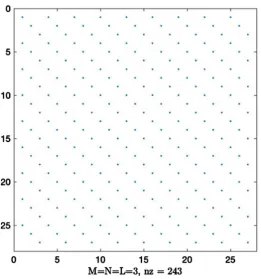
DOI: 10.4236/ajcm.2018.83018 225 American Journal of Computational Mathematics Figure 1. The sparse structure of SM⊗SN⊗IL with M N K= = =3.

3

M N K= = = , where

nz

means the number of the unknowns. Hence, the above equation can be transformed into a block tridiagonal matrix based on the structure of the fast operator. Equation (5) can be simplified as

(

)

(

)

(

)

, ,: , ,:

2 2 2

2 , ,:

2

, ,: , ,:

1

12 6

, 1,2, , ; 1,2, , .

12 i j i j

i L j L L i j L j L i L i j

i j i L j L L i j B B

k h _I _I _A h _I _A _A _k

h

F I I A F F i M j N

λ µ λ µ µ λ

λ µ

  

+ + + + + + + Φ

  

  

 

= + + + + − Φ =  = 

(6)

In this paper, we take Γ_{as the top surface of the domain and it can be} ex-tended to the general situations. Since the solutions on the other surfaces are al-ready known, we need to extract SB_top which contains the parts of

φ

i j L, , 1+ from

B

Φ _{, there follows}

(

)

(

)

( )

, ,

: :

, ,

, ,: 1 2 2 2 , , 1

2

, ,: ₁₂ , ,: i j 1i j ,

ij i j i j L i j L

i j i L j L L i j B B

P p p p a

h

F I I A F F

λ µ

+

Φ + + + Φ

+ + + + − Φ

= (7)

where

(

)

(

)

(

)

,

,,: ,:

2 2 2

2

2 2 2

T

1 2 2

(1)

2

,

1 ,

12 6

1

1 , , 0,0, ,1

2 6 .

1 ij i j top

ij i L j L L i j L j L i L L

B L

B B

k h h

P I I A I A A k I

k h h

S p p a

h

λ µ λ µ µ λ

 

= +_ _ + + + + + +

 

= Φ − = + = =

Φ 

(5)

First of all, constructing a LU-decomposition for Pij, i.e. P L Uij = ij ij, we have

(

)

(

)

( )

, ,: , ,:

, ,: 2 2 1 2 , , 1

2

, ,: ₁₂ , ,: i j 1i j .

ij ij i j i j L i j L

i j i L j L L ij B B

L U p p p a

h

F I I A F F

λ µ φ

λ µ

+

Φ + + +

= + + + + −Φ

(8)

Since 1

ij

L− _{is nonsingular, multiplying} 1

ij

L− _{on both side of Equation (8), we}

can obtain

(

)

(

)

( )

, ,: , ,:

1

, ,: 2 2 1 2 , , 1

2 1

, ,: ₁₂ , ,: i j 1i j .

ij i j i j ij L i j L

ij i j i L j L L i j B B

U p p p L a

h

L F I I A F F

λ µ φ

λ µ − + − Φ = + + +   + + + + −  

 Φ 

(9)

Consequently, the last equation of Equation (9) can be derived

, , , , 1 , , , 1,2, , ; 1,2, , ,

ij i j L ij i j L ri j L i M j N

α φ

+

β φ

+ = =  = 

₍₁₀₎

where

α

ij is the last element of Uij,

β

ij is the last element of

(

p2λi+p2µj+ p L1

)

⋅ ij La 2, and ri j L, , is the last element of

(

)

( ) ,: , ,: , 2 1 1

, ,: ₁₂ , ,: i j i j

ij i j h i L j L L i j B B

L F− ₊

λ

I ₊

µ

I ₊A F ₊F ₋_Φ _{. Combining} _{M N}_× _equations

analogously to Equation (10), we have

:,:,L :,:, 1L 1,

DαΦ +DβΦ + =R (11)

where

(

)

(

)

(

)

T

11 12 1 1 2

T

11 12 1 1 2

T

1 1,1, 1,2, 1, , 2,1, 2,2, 2, , ,1, ,2, , ,

diag , , , , , , , , ,

, , , , , , , , , , , , .

N M M MN

L L N L L L N L M L M L M N L

D D

R r r r r r r r r r

α β

α α α α α α

β β β β β β

= = =          

4. Discretization of Neumann Boundary Condition

The fourth-order finite difference discretization of Equation (2) can be ex-pressed as

( )

2

, , 2 , , 4

, , .

2 6

i j L i j L

zzz i j L

h _{O h}

n h

φ φ

φ + − _φ

∂

= − +

∂

Using the fourth-order substitution of φzzz we can derive

( )

2 2 2 2 2 2 2 2

2 2 2 2

, , 2 , ,

3

, , 1

1 1

6 6 6 6 6 6

2 , 1,2, , ; 1,2, , ,

3

x y i j L x y i j L

ij z i j L

k h h h k h h h

h

hg f i M j N

δ δ φ ₊ δ δ φ

+     + + + − + + +         = + = _ = _

or the matrix form

(

)

(

)

(

)

( )

2 2 2 2

2

:,:, 2 :,:,

3

:,:, 1. 1

6 6 6

2 3

MN M N M N L L B

z L

k h _I h _A _I h _I _A

h

hg f

+

  

+ + ⊗ + ⊗ Φ − Φ + Φ

(6)

( )

₍

₎

(

)

2 _T

2

0,1, 0,2, 0, , 1,1, 1,2, 1, ,

2 _T

1,0, 1, 1, 2,0, 2, 1, ,0, , 1,

, , , ,0,0, ,0, , , , ,

6

,0, , , ,0, , , , ,0, ,

6

B L L N L M L M L M N L

L N L L N L M L M N L

h b b b b b b

h b b b b b b

+ + + + + + Φ = +        

and bj j L, , =b x y z

(

i, ,j L

)

.

Multiplying SM ⊗SN on both side of Equation (12), we can obtain

(

)

(

)

(

)

( )

2 2 2 2

2

1 2 :,:, 2 :,:, 2

1 Λ ,

6 MN 6 N 6 M L L B

k h _I h _I h _I _R

+

  

+ + Λ ⊗ + ⊗ Φ − Φ = − Φ

  

  

  (13)

where

(

)

3

( )

( )2

₍

₎

( )2

2 M N 2 ₃ z :,:, 1L , B M N B

h

R = S ⊗S _ hg+ f ₊ _ Φ = S ⊗S Φ

  .

Moreover, replacing l with L+1_{in Equation (3), we have}

(

)

(

)

(

)

(

)

2 4 2 4 2 2

2 2 2 2 2 2

, , 1

2 2 2

2 2

, , 2 , ,

2

2 2 2 2 2 2 2

, , 1 , , 1

2 _{2 1}

12 3 6 12

1

12 6

, 12

x y x y i j L

x y i j L i j L

i j L x y x z y z i j L

k h h h _{k h} k h

k h h

h

h f f

δ δ δ δ φ

δ δ φ φ

δ δ δ δ δ δ

+ + + +     + + + + − +              + + + +  +        = _ + + + _   (14)

and the matrix form

(

)

(

)

(

)

(

)

( )

( ) ( )

(

)

2 4 2 4 2 2

:,:, 1

2 2 2

3 :,:, 2 :,:,

3 3

2

2 ₂ 5

12 3 6 6

1

12 6

,

M N M N M N MN L

MN M N M N L L B

B

k h h _A _I _I _A h _A _A k h _I

k h _I h _A _I _I _A

h F F

+

    

+ ⊗ + ⊗ + ⊗ − − Φ

    

    

 

  

+ +  + ⊗ + ⊗  Φ + Φ + Φ

     = + (15) where ( )

(

)

(

)

2 3 :,:, 1 2 2 :,:, 2 :,:, 2 12 12 6 6 .

M N M N M N MN L

M N M N L

h

F A A I A A I I F

h h I A A I F

h I A A I F

+ +   = _ ⊗ + ⊗ + ⊗ + _   − ⊗ + ⊗ − ⊗ + ⊗

Multiplying SM ⊗SN on both side of Equation (15), there follows

(

)

(

)

(

)

(

)

2 4 2 4 2 2

1 2 1 2 :,:, 1

2 2 2

1 2 :,:, 2 :,:, 3

2 _Λ _Λ _Λ _Λ ₂ 5

12 3 6 6

1 Λ Λ

12 6 ,

N M MN L

MN N M L L

k h h _I _I h k h _I

k h _I h _I _I _R

+

    

+ ⊗ + ⊗ + ⊗ − − Φ

    

    

 

  

+__ + _ + ⊗ + ⊗ _ Φ + Φ =

  

 

(16)

where 2

(

( )3 ( )3

)

3 B

(7)

Eliminating Φ:,:, 2L+ from Equation (13) gives

( )

(

2

)

1

:,:, 1L 2 :,:,L 3 2 B ,

C D R DB R−

+

Φ + Φ = − − Φ

(17) where

(

)

(

)

(

)

(

)

(

)

2 2 2 2

1 2

2 4 2 4 2 2

1 2 1 2

2 2 2

1 2

1 Λ ,

6 6 6

2 _Λ _Λ _Λ _Λ ₂ 5 _,

12 3 6 6

1 Λ Λ .

12 6

MN N M

N M MN

MN N M

k h h h

B I I I

k h h h k h

C I I I

k h h

D I I I

 

= +_ _ + Λ ⊗ + ⊗

 

   

=_ + _ ⊗ + ⊗ + ⊗ −_ − _

   

 

= +_ _ + ⊗ + ⊗

 

Combining Equation (11) and Equation (17) and derive a linear system

:,:, 1L ,

AΦ + =R

₍₁₈₎

where

( )

(

2

)

1 1 1

3 2 1

2 , B 2 .

A C= − DD D R R DB Rα− β = − − − Φ − DD Rα−

Finally, after deriving Φ:,:, 1L+ , we can obtain Φi j, ,: by substituting Φ:,:, 1L+ in

Equation (7). Multiplying SM⊗SN⊗IL, we can get the numerical solution of

the 3D Helmholtz equation.

5. Numerical Experiments

In this section, two numerical experiments are presented to test the validity and efficiency of the proposed method. Both experiments are implemented on MATLAB. All the equations are solved by the BiCG method. Equations in the two examples are solved in a cube Ω=

[ ] [ ] [ ]

0,1× 0,1× 0,1 _.

Example 1. Consider the following problem

(

)

( ) ( )

( )

(

)

(

)

sin π sin π

, , 2sinh 2π sinh 2π 1

sinh 2π

x y

u x y z = _ z + −z _₍₁₉₎

with

(

)

( ) ( )

(

)

( ) ( )

(

)

{ }

, , sin π sin π , 0, , , 2sin π sin π , 1, , , 0, 0,1 , 0,

u x y z x y z

u x y z y z

= =

 

= =



 ₌ _∈ ₌



0

f = _{and the corresponding Neumann boundary condition can be}

[image:7.595.206.540.77.368.2]

calcu-lated.

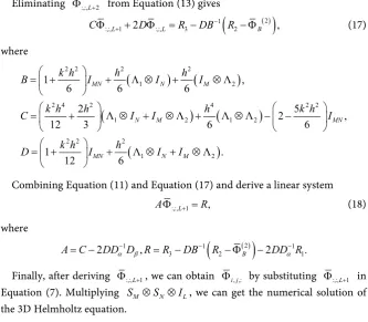
Table 1 fully corroborates the theoretical design rate of the convergence for the proposed method. We can see that a good accuracy (10−7_{) is achieved with a}

(8)

represent two different transform operators. As we can see from Table 1, the al-gorithm proposed in this paper saves much computational time and makes it possible to solve the equation with large grid number. Meanwhile, we give the numerical solutions of Equation (19) in the whole domain and numerical solu-tion on the face 1

2

z= in Figure 2 and Figure 3 respectively. Example 2.

(

)

( ) ( ) ( )

2 _{2π sin π sin π sin}2 _{, in ,}

0, on \ ,

u k u x y kz

u

+ = − Ω

= ∂Ω Γ

with the exact solution

( ) ( ) ( )

sin π sin π sin .

u= x y kz

₍₂₀₎

[image:8.595.208.539.325.705.2]

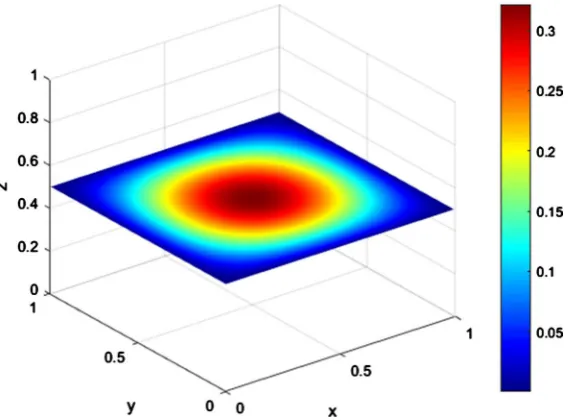
We give the figures of the numerical solutions U with different wave number in Figure 4 and Figure 5. As shown in Figure 4 and Figure 5, the solutions of the Helmholtz equation are highly oscillating for large wave number.

Table 1. Convergence rate and comparisons of computational time (s) for solving Exam-ple 1 with different operators.

M Solve U time (s) Memory (MB) Error Conv. rate

M N L

S ⊗S ⊗S SM⊗SN⊗SL

32 0.7556 0.5286 0.9472 7.4431e−07 − 64 28.5552 3.8459 6.7842 4.82273−08 3.9480 128 1051.3515 59.8049 51.1303 3.0654e−09 3.7223 256 46,725.7567 1013.8436 396.1303 1.9288e−10 4.2437 512 - 21,228.72458 3122.0200 1.1633e−11 4.0514

(9)

[image:9.595.158.446.70.280.2] [image:9.595.59.543.337.709.2]

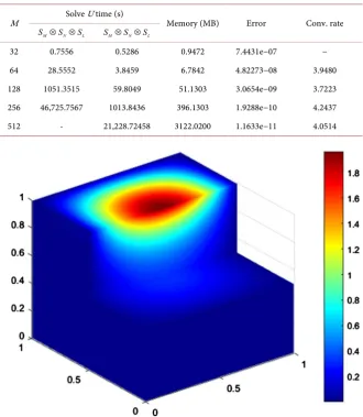
DOI: 10.4236/ajcm.2018.83018 230 American Journal of Computational Mathematics Figure 3. The numerical solutions of Equation (19) on the face z=1 2_with M =512_.

Figure 4. The numerical solutions of Equation (20) with k=3π_{(left) and} k=5π_(right).

[image:9.595.57.544.520.702.2]

(10)

6. Conclusion

We propose a fast-high order method for solving the 3D Helmholtz equation with Neumann boundary condition. Fourier operator is used to generate block-tridiagonal structure of the discretization of the Helmholtz equation. Moreover, by using the Gaussian elimination in the vertical direction, the Helmholtz equation is reduced into a linear system in the layer of the domain. The validity and efficiency of the method are tested by two numerical experi-ments.

Acknowledgements

This research was supported by the Nature Science Foundation of Hebei Prov-ince (No. A2016502001) and the Fundamental Research Funds for the Central Universities (No. 2018MS129).

Conflicts of Interest

The authors declare no conflicts of interest regarding the publication of this pa-per.

References

[1] Singer, I. and Turkel, E. (1998) High-Order Finite Difference Methods for the Helmholtz Equation. Computer Methods in Applied Mechanics & Engineering, 163, 343-358. https://doi.org/10.1016/S0045-7825(98)00023-1

[2] Harari, I. and Hughes, T.J.R. (1991) Finite Element Methods for the Helmholtz Equation in an Exterior Domain: Model Problems. Computer Methods in Applied Mechanics & Engineering, 87, 59-96.

https://doi.org/10.1016/0045-7825(91)90146-W

[3] Jin, J.M., Liu, J., Lou, Z. and Liang, C.S.T. (2003) A Fully High-Order Fi-nite-Element Simulation of Scattering by Deep Cavities. Antennas & Propagation IEEE Transactions on, 51, 2420-2429. https://doi.org/10.1109/TAP.2003.816354 [4] Jin, J.M. and Liu, J. (2000) A Special Higher Order Finite-Element Method for

Scat-tering by Deep Cavities. IEEE Transactions on Antennas & Propagation, 48, 694-703. https://doi.org/10.1109/8.855487

[5] Braverman, E., Israeli, M. and Averbuch, A. (1999) A Fast Spectral Solver for a 3D Helmholtz Equation. Society for Industrial and Applied Mathematics, 20, 2237-2260. https://doi.org/10.1137/S1064827598334241

[6] Nabavi, M., Siddiqui, M.H.K. and Dargahi, J. (2007) A New 9-Point Sixth-Order Accurate Compact Finite-Difference Method for the Helmholtz Equation. Journal of Sound & Vibration, 307, 972-982. https://doi.org/10.1016/j.jsv.2007.06.070 [7] Hong, P.L., Minh, T.L. and Hoang, Q.P. (2018) On a Three Dimensional Cauchy

Problem for Inhomogeneous Helmholtz Equation Associated with Perturbed Wave Number. Journal of Computational and Applied Mathematics, 335, 86-98. https://doi.org/10.1016/j.cam.2017.11.042

(11)

DOI: 10.4236/ajcm.2018.83018 232 American Journal of Computational Mathematics https://doi.org/10.1016/j.enganabound.2017.06.005

[9] Kashirin, A.A., Smagin, S.I. and Taltykina, M.Yu. (2016) Mosaic-Skeleton Method as Applied to the Numerical Solution of Three-Dimensional Dirichlet Problems for the Helmholtz Equation in Integral Form. Computational Mathematics and Mathematical Physics, 56, 612-625. https://doi.org/10.1134/S0965542516040096 [10] Britt, S., Tsynkov, S. and Turkel, E. (2010) A Compact Fourth Order Scheme for the

Helmholtz Equation in Polar Coordinates. Journal of Scientific Computing, 45, 26-47. https://doi.org/10.1007/s10915-010-9348-3

[11] Ortega, G., García, I. and Garzón, G.E.M. (2013) European Conference on Parallel Processing: A Hybrid Approach for Solving the 3D Helmholtz Equation on Hetero-geneous Platforms. Springer, Berlin, 8374, 198-207.

[12] Sutmann, G. (2007) Compact Finite Difference Schemes of Sixth Order for the Helmholtz Equation. Journal of Computational & Applied Mathematics, 203, 15-31. https://doi.org/10.1016/j.cam.2006.03.008

[13] Shaw, R.P. (2000) Integral Equation Methods in Acoustics. Boundary Elements, 4, 221-244.

[14] Poulson, J., Engquist, B., Li, S.W. and Ying, L.X. (2013) A Parallel Sweeping Pre-conditioner for Heterogeneous 3D Helmholtz Equations. SIAM Journal on Scien-tific Computing, 35, 194-212. https://doi.org/10.1137/120871985

[15] Singer, I. and Turkel, E. (2006) Sixth-Order Accurate Finite Difference Schemes for the Helmholtz Equation. Journal of Computational Acoustics, 14, 339-351. https://doi.org/10.1142/S0218396X06003050

[16] Boisvert, R.F. (1985) A Fourth-Order-Accurate Fourier Method for the Helmholtz Equation in Three Dimensions. ACM Transactions on Mathematical Software, 13, 221-234. https://doi.org/10.1145/29380.29863

[17] Li, C.L. and Zou, J.W. (2013) A Sixth-Order Fast Algorithm for the Electromagnetic Scattering from Large Open Cavities. Applied Mathematics and Computation, 219, 8656-8666. https://doi.org/10.1016/j.amc.2013.02.014