Generalized Thermoelasticity Problem of Material Subjected to Thermal Loading Due to Laser Pulse

Generalized Thermoelasticity Problem of Material

Subjected to Thermal Loading Due to Laser Pulse

Hamdy M. Youssef1,2, Ahmed S. Al-Felali3

1_{Mechanical Department, Faculty of Engineering and Islamic Architecture, Umm Al-Qura University, Makkah, Saudi Arabia} 2_{Mathematics Department, Faculty of Education, Alexandria University, Alexandria, Egypt}

3_{Mathematical Department, Faculty of Sciences, Umm Al-Qura University, Makkah, Saudi Arabia} Email: [email protected]

Received November 18, 2011; revised December 29, 2011; accepted January 7, 2012

ABSTRACT

This work is devoted to a study of the induced temperature and stress fields in an elastic half space in context of classi-cal coupled thermoelasticity and generalized thermoelasticity in a unified system of equations. The half space is consid-ered to be made of an isotropic homogeneous thermoelastic material. The bounding plane surface is heated by a non- Gaussian laser beam with pulse duration of 2 ps. An exact solution of the problem is first obtained in Laplace transform space. Since the response is of more interest in the transient state, the inversion of Laplace transforms have been carried numerically. The derived expressions are computed numerically for copper and the results are presented in graphical form.

Keywords: Thermoelasticity; Coupled Thermoelasticity; Generalized Thermoelasticity; Non-Gaussian Laser Pulse

1. Introduction

Although thermomechanical phenomena in the majority of practical engineering applications are adequately si- mulated with the classical Fourier heat conduction equa- tion, there is an important body of problems that require due consideration of thermomechanical coupling: it is appropriate in these cases to apply the generalized theory of thermoelasticity. Serious attention has been paid to the generalized thermoelasticity theories in solving thermoe-lastic problems in place of the classical uncoupled/cou- pled theory of thermoelasticity.

The absence of any elasticity term in the heat conduc-tion equaconduc-tion for uncoupled thermoelasticity appears to be unrealistic, since due to the mechanical loading of an elastic body, the strain so produced causes variation in the temperature field. Moreover, the parabolic type of the heat conduction equation results in an infinite velocity of thermal wave propagation, which also contradicts the actual physical phenomena. Introducing the strain-rate term in the uncoupled heat conduction equation, Biot extended the analysis to incorporate coupled thermoelas-ticity [1]. In this way, although the first shortcoming was over, there remained the parabolic type partial differen-tial equation of heat conduction, which leads to the pa-radox of infinite velocity of the thermal wave. To elimi-nate this paradox generalized thermoelasticity theory was developed subsequently. Due to the advance-

ment of pulsed lasers, fast burst nuclear reactors and par-ticle accelerators, etc. which can supply heat pulses with a very fast time-rise [2,3]; generalized thermoelasticity theory is receiving serious attention. The development of the second sound effect has been nicely reviewed by Chandrasekharaiah [4]. At present mainly two different models of generalized thermoelasticity are being exten-sively used-one proposed by Lord and Shulman [5] and the other proposed by Green and Lindsay [6]. L-S (Lord and Shulman theory) suggests one relaxation time and according to this theory, only Fourier’s heat conduction equation is modified; while G-L (Green and Lindsay theory) suggests two relaxation times and both the en-ergy equation and the equation of motion are modified.

tion time,Sherief and Anwar [9] have obtained the dis-tributions of thermal stresses and temperature for a gen-eralizedthermoelastic problem in which an infinite elastic space was subjected to the influence of a continuous linesource of heat. The solution of the problem was ob-tained by applying the Hankel and Laplace integral transformssuccessively. Wang and Xu have studied the stress wave induced by nanoseconds, picoseconds, and femtoseconds laser pulses in a semi-infinite solid [10]. The solution takes into account the non-Fourier effect in heatconduction and the coupling effect between tem-perature and strain rate. It is known that characteristic elasticwaveforms are generated when a pulsed laser irra-diates a metal surface. Point in case, McDonald hasstud-ied the importance of thermal diffusion to the thermoe-lastic wave generation [11]. Bagri and Eslami got the unified generalized thermoelasticity solution for cylinders and spheres [12].

The present investigation is devoted to a study of the induced temperature and stress fields in an elastic half space under the purview of classical coupled thermoelas- ticity and generalized thermoelasticity in a unified sys- tem of field equations. The half space continuum is con- sidered to be made of an isotropic homogeneous ther- moelastic material, the bounding plane surface being sub- jected to a Non-Gaussian laser pulse. An exact solution of the problem is first obtained in Laplace transform space. Since the response is of more interest in the tran- sient state, the inversion of Laplace transforms have been carried numerically. The derived expressions are com- puted numerically for copper and the results are pre- sented in graphical form.

2. Basic Equations and Formulation

All the field equations represented by (CTE), (L-S) and (G-L) can be formulated in the following unified system [13] and [14]:





, , 1

i i jj j ji i

u u u F

t

      _  



 

 _T_,i, (1)

which constitute equation of motion where  , are Lame’s constants, ui is the displacement component,

F is the body force component, _T

i



3 2



    and

T

 is the thermal expansion,  is relaxation time, T is

the temperature of the body and  is the density.





2

, 2

,

1 ,

ii E o

o o j j

K T C T

t t

n T u Q

t

 

  

   

 _  _

 

 

  

 _{ } 



  

(2)

which constitute equation of heat conduction where K is

the thermal conductivity, CE is the specific heat at

con-stant strain, o is relaxation time, To is the reference

temperature, n is a parameter and Q is the heat source.



, ,



,



ij ui j uj i ui i T T



ij

   _   _ _{. (3)}

which is called constitutive equation where ij is the

stress tensor and ij is the Kronecker function.

Equations (1)-(3) reduce to coupled thermoelasticity (CTE) when o   0 . Putting n1 , 0 and

0

o

  , the equations reduce to Lord-Shulman (L-S) model, while when n0, _o0 and 0, the eq-uations reduce to Green-Lindsay (G-L) model [13,14].

3. The Non-Gaussian Laser Pulse

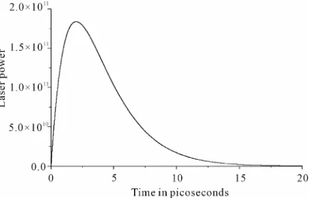
We will consider the medium is heated uniformly by a laser pulse with non-Gaussian form temporal profile [7].

 

0

2 exp

p p

L t t

L t

t t

 

 _

  , (4)

where tp 2 ps is a characteristic time of the laser- pulse (the time duration of a laser pulse), L0 is the laser intensity which is defined as the total energy carried by a laser pulse per unit area of the laser beam, see Figure 1, [7].

The conduction heat transfer in the medium can be modeled as a one-dimensional problem with an energy source Q x t

 

, near the surface, i.e.

 

 

0 2

1 / 2

, exp

/ 2

exp ,

a

p p

R x h

Q x t I t

R L x h t

t

t t

 

 

   

 _{ }

 

 _ 

 _  _

 

(5)

where  is the absorption depth of heating energy and

Ra is the surface reflectivity [7].

[image:2.595.312.538.572.717.2]

When we consider the laser pulse lie on the surface of the mediumwhen x0 (see Figure 1), we get the en-ergy source in the form

 

0

2 exp ₂

a

p p

R L h t

Q t t

t t   _   _    

. (6)

4. Formulation of the Problem

We consider half-space ( ) with the x-axis pointing into the medium with initial temperature distribution To.

This half-space is irradiated uniformly the bounding plane (x = 0) by a laser pulse with non-Gaussian

tempo-ral profile as in (6). We assume that there is no body forces affecting the medium and all the state functions initially are equal to zero.

0

x

The displacement vector has the components:

 

, , 0

uu x t vw . (7)

Hence, the governing Equations (1)-(3) in one-dimen- sional will take the following forms:

The equation of motion



2



22 1

u u x t x        _        

 _ , (8)

where  T T_o is the temperature increment.

The heat equation:

2 2 0 0 0 2 2 0 0 2

1 exp ,

2 E a p p T C n e

K t K t

x t

R L h t

n t

t K t t

   _{  }              _  _  _     _  _{ }       _  _ _  _    _{ } 2 2 t     (9) where u e x  

 . (10)

The constitute equation:



2



1

xx e t     _      

 . (11)

For simplicity, we will use the following non-dimen- sional variables Youssef (2006):





















0 2

0 0 0

, , , , , , , , , , , , , , , . 2 2 p p ij ij

x u h c x u h

t t c t t

                                (12)

wherec_o  2





 is the longitudinal wave speed

and CE

K



 is the thermal viscosity.

Hence, we have the following system of equations (we

have dropped the prime for convenient)

2 2

2 2 1

e e

t

x x  

 

  

  _ 



 _{  }

 _ , (13)

2 2

0 1 0

2 2

2 0

1 exp ,

p n e t t x t t n t t t  _{   }   2 2 t         _  _  _      _  _{ }         _  _ _ _    _{ }  (15) 1 xx e t    _       



, (16)

where



2 0 1 ₂ E T C      

 is the dimensionless thermoe-

lastic coupling constant, and 0

2 2 exp ₂

a

p o

R L h

t K c

       _{ }  .

5. The Exact Solution of the Problem in the

Laplace Transform Domain

Applying the Laplace transform for Equations (13)-(15) defined by the formula

 

 

 

0

e dst

f s L f t f t t

 

 _ _

_

.

Hence, we obtain the following system of differential equations



2 2



_e



₁



2

x

D s  s Dx , (17)









 

2 2 2

0 1 0 e

x

D s  s   s n s F s

 _{ }  _{  }

  , (18)





e 1

xx s

     , (19) where all the state functions initially are equal to zero,

d d n n x n D x

 and

 







2 0



2 1 1/ _p n s F s s t      .

Eliminating e between the Equations (17) and (18), we get

 



4 2

2

4 2

d d _,

dx Ldx M  x s s F

 

  

 

  s



, (20)

where 2



2

 

2





1 1

o o

Ls  s  s  sn s s



and





2 2

o

M s s s .

The solution of Equation (20) takes the following form:

 

 

2



2 2





2 1

, _{i i} e _i

i o

F s



xp

x s A s

s s x

  

 

   





. (21)

equation

4 2 ₀

L M

     , (22) and

  



2 2



1

, 1 i i exp i

i

e x s s A x





 



 . (23)

To get the value of the parameters A₁ and A₂ we

have to apply the boundary conditions on the bounding plane x0 of the assumed half space as follows:

   

0,t e 0,t 0

   , (24)

which gives after applying Laplace transform

 

0,s e

 

0,s 0

  



. (25)

After applying the above boundary conditions, we get

 



 

2 2

1 _{2 2 2 2}

2 1

o

F s A

s s s



  



 

and

 



 



2 1

2 _{2 2 2 2}

2 1

.

o

F s A

s s s



  

 

 

Finally, we can write the solution in the Laplace transform domain as follows:

 

 









 1





 

2 2 2 2

2 1

2 2 2 2 2 2

1 2 2 1

1

, 1

e e ,

o

x

F s x s

s s s

s  s



  

    



  

 _ 



2x 

 



_    _

 

(26)

and

 

_

 

_{ }



_

 1  2 

2 2

1 2

2 2 2 2

2 1

1

, e x

o

F s s

e x s

s s s

 

  

  

 

 _{ }

 _  _

  e

x _{. (27)}

By using Equations (19), (26) and (27), we get

 











 1  2 

2

2 2

2 1

2 2

2 1

1

1

e e 1 .

xx

o

x x

F s s

s s

 

 



 

 

 

 



 

 

 

 _  _

  

 



(28)

We get the displacement form Equations (10) and (27) in the form

 

 





₂

 

_{2 2} 1 2₂



2  1 1  2 

2 1

1

, e x e x

o

F s s

u x s

s s s

 

  

 

  

 

  _{ }

 _  _

  .

(29)

6. Numerical Results

In order to get the inversion of the Laplace transform, the Riemann-sum approximation method is used. In this me- thod, any function in Laplace domain can be inverted to the time domain as

 

 

 

1

e 1 π

1 2

t N

n n

i n

g t g Re g

t t



 



  

 _   _  _

 





, (30)

where Re is the real part and is imaginary number

unit. For faster convergence, numerous numerical expe- riments have shown that the value of satisfies the re- lation

i



κt4.7 [8].

With a view to illustrating the analytical procedure presented earlier, we now consider a numerical example for which computational results are given. For this pur-pose, copper is taken as the thermoelastic material, [13]:

1 3

386 kg m k s

K      ,_T 1.78 10

 

5k1 ,T_o293k

3 8954 kg m

_{ } 

E

C

, _{383.1 m k}2_ 1_s2

10 1 2

86 10 kg m s, ,

11 2

0 1 10 J/m

L   3.   

2 ,

10 1

7.76 10 kg m s

_{  }  _  _0.5

a

R  h0.1,

, ,  0.01,

2.0

p

t  , o 0.02, 0.08, 10.0168, .

4 2 2.1 10

  

The computations were carried out for t = 0.2 and the

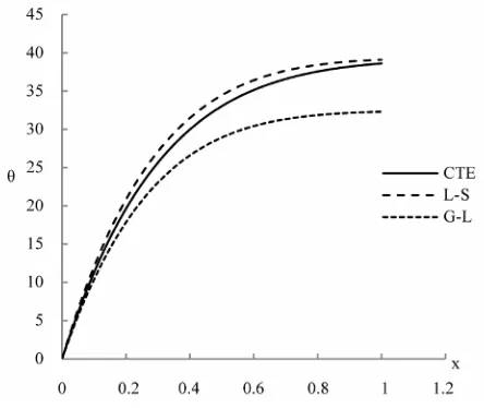
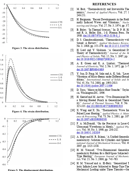
temperature, the stress, the strain and the displacement distributions are represented graphically at different posi-tions of x.

The Figures 2-5 show that, the laser pulse makes the difference between the results in the context of the three studied models CTE, L-S and G-L is very clear and we can differentiate between them, while it was very diffi-cult previously when we used thermal loading by using thermal shock or ramp-type heating as in [13,14].

7. Acknowledgements

[image:4.595.312.534.533.720.2]

The authors are grateful for the supports for this work

REFERENCES

[1] M. Boit, “Thermoelasticity and Irreversible Thermo-Dy- namics,” Journal of Applied Physics, Vol. 27, 1956, pp. 240-251.

[2] H. Bargmann, “Recent Developments in the Field of Ther- mally Induced Waves and Vibrations,” Nuclear Engi- neering and Design, Vol. 27, No. 3, 1974, pp. 372-381.

[3] B. Boley, “In Thermal Stresses,” In: D. P. H. Hasselman and R. A. Heller, Eds., 1-ll. Plenum Press, New York, 1980. doi:10.1007/978-1-4613-3156-8_1

[4] D. S. Chandrasekharaiah, “Thermoelasticity with Second Sound: A Review,” Applied Mechanics Review, Vol. 39

[image:5.595.68.507.77.657.2]

No. 3, 1986, pp. 355-376. doi:10.1115/1.3143705 Figure 3. The stress distribution.

[5] H. Lord and Y. Shulman, “A Generalized Dynamical Theory of Thermoelasticity,” Journal of the Mechanics and Physics of Solids, Vol. 15, No. 5, 1967, pp. 299-307.

doi:10.1016/0022-5096(67)90024-5

[6] A. E. Green and K. A. Lindsay, “Thermoelasticity,”

Journal of Elasticity, Vol. 2, No. 1, 1972, pp. 1-7.

doi:10.1007/BF00045689

[7] Y. Sun, D. Fang, M. Saka and A. K. Soh, “Laser-Induced Vibrations of Micro-Beams under Different Boundary Con- ditions,” International Journal of Solids and Structures,

Vol. 45, No. 7-8, 2008, pp. 1993-2013. doi:10.1016/j.ijsolstr.2007.11.006

[8] D. Tzou, “Macro-to-Micro Heat Transfer,” Taylor & Fran- cis, Washington DC, 1996.

[9] H. Sherief and M. Anwar, “Two-Dimensional Problem of a Moving Heated Punch in Generalized Thermoelastic-ity,” Journal of Thermal Stresses, Vol. 9, No. 4, 1986,

325-335. doi:10.1080/01495738608961910

[10] X. Wang and X. Xu, “Thermoelastic Wave Induced by Pulsed Laser Heating,” Applied Physics A: Materials Sci- ence & Processing, Vol. 73, No. 1, 2001, pp. 107-114.

doi:10.1007/s003390000593 Figure 4. The strain distribution.

[11] F. A. McDonald, “On the Precursor in Laser-Generated Ultrasound Waveforms in Metals,” Applied Physics Let-ters, Vol. 56, No. 3, 1990, pp. 230-232.

doi:10.1063/1.102839

[12] A. Bagri and M. R. Eslami, “A Unified Generalized Ther- moelasticity; Solution for Cylinders and Spheres,” Inter-national Journal of Mechanical Sciences, Vol. 49, No. 12,

2007, pp. 1325-1338.

[13] H. M. Youssef, “Two-Dimensional Generalized Ther-moelasticity Problem for a Half-Space Subjected to Ramp- Type Heating,” European Journal of Mechanics—A/So- lids, Vol. 25, No. 5, 2006, pp. 745-763.

[14] H. M. Youssef and A. El-Bary, “Generalized Thermoe-lastic Infinite Layer Subjected to Ramp-Type Thermal and Mechanical Loading under Three Theories—State Space Approach,” Journal of Thermal Stresses, Vol. 32, No. 12,

2009, pp. 1293-1310. doi:10.1080/01495730903249276 Figure 5. The displacement distribution.

[image:5.595.64.299.87.640.2]