Modeling and Performance Analysis of Weighted Priority Queueing for Packet Switched Networks

(1)

ISSN Print: 2327-5219

DOI: 10.4236/jcc.2018.611019 Nov. 23, 2018 195 Journal of Computer and Communications

Modeling and Performance Analysis of

Weighted Priority Queueing for

Packet-Switched Networks

Dariusz Strzeciwilk

1

_{, Wlodek M. Zuberek}

2

1_{University of Life Sciences, Department of Applied Informatics, Warsaw, Poland}

2_{Memorial University, Department of Computer Science, St. John’s, Canada}

Abstract

Weighted priority queueing is a modification of priority queueing that elimi-nates the possibility of blocking lower priority traffic. The weights assigned to priority classes determine the fractions of the bandwith that are guaranteed for individual traffic classes, similarly as in weighted fair queueing. The paper describes a timed Petri net model of weighted priority queueing and uses dis-crete-event simulation of this model to obtain performance characteristics of simple queueing systems. The model is also used to analyze the effects of fi-nite queue capacity on the performance of queueing systems.

Keywords

Timed Petri Nets, Discrete-Event Simulation, Priority Queueing, Weighted Priority Queueing, Performance Analysis

1. Introduction

Although the internet was originally intended for non-time-critical transport

[1], there is a growing interest in adding real-time traffic to the traditional non-time-critical bulk traffic. Real-time traffic is characterized by bounds on some performance metrics (such as delay, jitter or packet loss probability). Voice over IP (VoIP) and Internet Protocol TV (IPTV) are examples of real-time traf-fic. Because of these performance bounds, real-time traffic requires preferential service during transport.

The strategy for mixing real-time and bulk traffic is to use, at the nodes of the network, separate queues for different classes of traffic, so the real-time traffic can get the service it requires. Priority queueing [2] is the simplest mechanism

How to cite this paper: Strzeciwilk, D. and Zuberek, W.M. (2018) Modeling and Per-formance Analysis of Weighted Priority Queueing for Packet-Switched Networks. Journal of Computer and Communications, 6, 195-208.

https://doi.org/10.4236/jcc.2018.611019

Received: October 10, 2018 Accepted: November 20, 2018 Published: November 23, 2018

http://creativecommons.org/licenses/by/4.0/

(2)

DOI: 10.4236/jcc.2018.611019 196 Journal of Computer and Communications

that provides preferential service to some classes of traffic; in the priority queueing, lower priority traffic can be serviced only when all queues of higher priority classes are empty. Such a policy works well when the traffic is not very intensive but can result in blocking lower priority traffic for extended periods of time if the traffic in higher priority classes becomes intensive. Therefore a num-ber of modifications of (strict) priority queueing were proposed to avoid such blocking and to guarantee some levels of service for lower priority classes inde-pendently of traffic in higher priority classes [3], [4]. Weighted priority queueing is one of such modifications which assigns fractions of the bandwidth to traffic classes according to class weights.

Modern communication networks [5] are complex structures which—for modeling—require a flexible formalism that can easily handle concurrent activi-ties as well as synchronization of different events and processes that occur in such networks [6]. Petri nets [7], [8] are such formal models. As formal models, Petri nets are bipartite directed graphs, in which the two types of vertices represent, in a very general sense, conditions and events. An event can occur only when all conditions associated with it (represented by arcs directed to the event) are satisfied. An occurrence of an event usually satisfies some other con-ditions, indicated by arcs directed from the event. So, an occurrence of one event causes some other event to occur, and so on.

In inhibitor Petri nets, in addition to directed arcs, inhibitor arcs provide “test if zero” condition which does not exist in “standard” Petri nets. Inhibitor arcs are needed for modeling priority mechanisms.

In order to study performance aspects of systems modeled by Petri nets, the durations of modeled activities must also be taken into account. This can be done in different ways, resulting in different types of temporal nets. In timed Pe-tri nets [9], occurrence times are associated with events, and the events occur in real-time (as opposed to instantaneous occurrences in other models). For timed nets with constant or exponentially distributed occurrence times, the state graph of a net is a Markov chain (or an embedded Markov chain), in which the statio-nary probabilities of states can be determined by standard methods [10]. These stationary probabilities are used for the derivation of many performance charac-teristics of the model.

Timed Petri nets are used in this paper to develop models of weighted priority queueing and then performance characteristics of simple queueing systems are obtained by discrete-event simulation of developed models.

Section 2 recalls basic concepts of Petri nets and timed Petri nets. Section 3 describes the net model of weighted priority queueing while Section 4 uses the developed model to analyze the performance of simple weighted priority queue-ing systems. Section 5 concludes the paper.

2. Petri Nets and Timed Petri Nets

(3)

Computer systems, communication networks, manufacturing systems and transportation systems are examples of such systems. Concurrent activities are represented in Petri nets by tokens which can move within a (static) graph-like structure of the net. More formally, a marked inhibitor place/transition Petri net

 is defined as a pair =

(

,m0

)

, where the structure  is a bipartite

directed graph,  =

(

P T A H, , ,

)

with the two types of vertices being a set of places P and a set of transitions T, and a set of directed arcs A which connect places with transitions and transitions with places, A T P P T⊆ × _ × _{, while}_H

is a set of inhibitor arcs which connect places with transitions, H P T⊂ × _;

usually A H = ∅. Finally, m0 is the initial marking function which assigns

nonnegative numbers of tokens to places of the net, m P0: →

{

0,1,

}

. Places

which are assigned nonzero numbers of tokens by a marking function m are called marked places, while places with zero tokens are called unmarked places. Marked nets can be equivalently defined as =

(

P T A H m, , , , 0

)

.

In Petri nets the distribution of tokens over places changes by occurrences (or firings) of transitions. A transition t is enabled by a marking function m if all places connected to t by directed arcs are marked and all places connected to t by inhibitor arcs are unmarked. When an enabled transition t occurs (or fires), one token is removed from each place connected to t by a directed arc and one to-ken is deposited to each place connected to t by an outgoing arc. An occur-rence of a transition creates a new marking function, a new set of enables transi-tions, and so on. The set of all marking functions that can be created starting from the initial marking m0 is called the reachability set of a net. This set can

be finite or infinite.

A place is shared if it is connected to more than one transition. A shared place

p is free-choice if the sets of places connected by directed arcs and inhibitor arcs to all transitions sharing p are identical. All transitions sharing a free-choice place constitute a free-choice class of transitions. For each marking function, ei-ther all transitions in each free-choice class are enabled or none of these transi-tions is enabled. It is assumed that a choice of an occurring transition in each free-choice class is random and can be described by probabilities associated with transitions. A shared place which is not free-choice is a conflict place and transi-tions sharing it are conflicting transitransi-tions.

(4)

in-DOI: 10.4236/jcc.2018.611019 198 Journal of Computer and Communications

itiated, which will overlap with the other occurrence(s). There is no limit on the number of simultaneous occurrences of the same transition (sometimes this is called infinite occurrence semantics). Similarly, if a transition is enabled “several times” (i.e., it remains enabled after initiating an occurrence), it may start several independent occurrences in the same time instant.

Formally, a timed Petri net is a triple,  =

(

, ,c f

)

, where  is a marked net, c is a choice function which assigns probabilities to transitions in free-choice classes and relative frequencies of occurrences to conflicting transitions,

[ ]

0,1

c→ _{, and} f is a timing function which assigns an (average) occurrence time to each transition of the net, f T: _→_R+_{, where} _R+_{is the set of}

nonneg-ative real numbers.

The occurrence times of transitions can be either deterministic or stochastic (i.e., described by some probability distribution function); in the first case, the corresponding timed nets are referred to as D-timed nets [13], in the second, for the (negative) exponential distribution of firing times, the nets are called M-timed nets (Markovian nets) [14]. In both cases, the concepts of state and state transitions have been formally defined and used in the derivation of differ-ent performance characteristics of the model. In simulation applications, other distributions can also be used, for example, the uniform distribution (U-timed nets) is sometimes a convenient option. In timed Petri nets different distribu-tions can be associated with different transidistribu-tions in the same model providing flexibility that is used in simulation examples that follow.

In timed nets, it is convenient to have a possibility of some events to occur “immediately”, i.e., in zero time; all transitions with zero occurrence times are called immediate (while the others are called timed). Since the immediate transi-tions have no tangible effects on the (timed) behavior of the model, it is conve-nient to “split” the set of transitions into two parts, the set of immediate and the set of timed transitions, and to first perform all occurrences of the (enabled) immediate transitions, and then (still in the same time instant), when no more immediate transitions are enabled, to start the occurrences of (enabled) timed transitions. It should be noted that such a convention effectively introduces the priority of immediate transitions over the timed ones, so the conflicts of imme-diate and timed transitions are not allowed in timed nets. Detailed characteriza-tion of the behavior or timed nets with immediate and timed transicharacteriza-tions is given in [9].

3. Weighted Priority Queueing

(5)

Weighted priority scheduling limits the number of consecutive packets of the same class that can be transmitted over the channel; when the scheduler reaches this limit, it switches to the next nonempty priority queue and follows the same rule. These limits are called weights, and are denoted w1. With k classes of

traf-fic, if there are sufficient numbers of packets in all classes, the scheduler selects

1

w packets of class 1, then w2 packets of class 2, …, then wk packets of class

k, and again w1 packets of class 1, and so on. Consequently, in such a situation

(i.e., for sufficient supply of packets in all classes), the channel is shared by the packets of all priority classes, and the proportions are:

1, ,

, 1, 2, ,

i i i

j j

j k

w s

u i k

w s

=

= =

∑



where s ii, =1, , k is the transmission rate for packets of class i. If the

trans-mission rates are the same for packets of all classes (as is assumed for simplicity in the illustrating examples), the proportions are:

1, ,

, 1, , .

i i

j

j k

w

u i k

w

=

= =

∑



For an example with 3 priority classes and the weights equal to 4, 2 and 1 for classes 1, 2 and 3, respectively, these “utilizations bounds” are equal to 4/7, 2/7 and 1/7, for classes 1, 2 and 3, respectively.

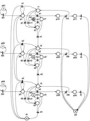
A Petri net model of weighted priority scheduling for three classes of packets with weights 4, 2 and 1 is shown in Figure 1. The model is composed of three identical interconnected sections corresponding to the three priority classes.

The main elements of the model are the three queues represented by places

1

p, p2 and p3 for traffic class 1, 2 and 3, respectively, and timed transitions 1

t , t2 and t3 modeling the transmission of selected packets through the

communication channel. The three classes of packets are generated (indepen-dently) by transitions t01, t02 and t03 with places p01, p02 and p03. The

occurrence times f t

( )

01 , f t

( )

02 and f t

( )

03 determine the arrival rates for

queues 1, 2 and 3, respectively.

The scheduling is based on repeated selection of queues in order of priorities (first class 1, then 2, and so on) for the transmission of queued packets. This se-lection operation is represented by a loop with places r0, r1, r2 and r3, and

1

q , q2 and q3. There is a single “control token” in this loop (shown in place 0

r in Figure 1). This token indicates the queue that is used for transmission of packets (by the subscript 1, 2 or 3); a token in place r0 indicates that no queue

is selected.

Let r0 be marked. If all three queues are empty, the next packet arriving to

one of the queues enables one of the transitions s1, s2 or s3, the control

to-ken is moved from r0 to place ri corresponding to the nonempty queue, and

an occurrence of transition ai selects a token from pi for transmission. At

the same time, one token from place wi is moved to place ui. When the

(6)

DOI: 10.4236/jcc.2018.611019 200 Journal of Computer and Communications • _{if the queue (place}p_i) is nonempty and the weight (wi) is nonempty,

another token is selected from pi and forwarded for transmission;

• _{if the queue is empty, an occurrence of transition} d_i moves the control to-ken from ri to qi;

• _{if the weight is empty, an occurrence of transition} c_i also moves the control token from ri to qi.

A token in qi moves (by repeated occurrences of bi) all tokens from place i

u back to wi, and when ui becomes empty, an occurrence of transition ei

moves the control token to the next class represented by ri+1. If the queue for

this class is empty, occurrences of transitions di+1 and ei+1 move the control

token to a subsequent class until r0 is reached, and then the highest priority

nonempty class is selected by an occurrence of one of transitions s1, s2 or 3

[image:6.595.214.530.274.695.2]

s .

(7)

The model shown in Figure 1 needs to be modified slightly to represent finite queues. The modifications are identical for all traffic classes, and are shown in

Figure 2 for class 1.

The (finite) capacity of the queue is represented by the initial marking of place

14

p (shown in Figure 2 as K). When a packet is generated (by t01) and the

queue is not full, i.e., place p14 is marked, an occurrence of t14 enqueues the

packet in p1. If, however, the queue is full, place p14 is unmarked, the

inhibi-tor arc

(

p t14 15,

)

enables t15 and the packet is dropped.

Finally, when a packet is selected for transmission and is removed from the queue, each occurrence of transition t10 returns a token to p14, indicating that

the queue can store another packet.

4. Performance Characteristics

The model shown in Figure 1 (three classes of traffic, weights 4-2-1) is used for performance analysis of weighted priority queueing. The utilizations of the shared communication channel as functions of traffic intensity of class 1 (the highest priority), ρ1, with constant traffic intensities for classes 2 and 3,

2 0.5

ρ = and ρ =3 0.25, is shown in Figure 3.

For ρ ≤1 0.25, channel utilizations for classes 2 and 3 are constant at the

le-vels of 0.5 and 0.25, respectively (all service rates are equal to 1 for simplicity, so the utilizations are equal to traffic intensities and also the arrival rates are equal to traffic intensities); for class 1, the utilization changes linearly with ρ1. It

should be noted that traffic intensities ρ2 and ρ3 are significantly greater that

the performance levels guaranteed by the weights 4-2-1 (equal to 2/7 and 1/7 for classes 2 and 3, respectively). For ρ =1 0.25, the channel becomes fully utilized

(ρ1+ρ2+ρ3 =1), so further increases of ρ1 result in decreasing utilizations of

the channel for classes 2 and 3, until the levels guaranteed by the weights are reached (these levels are 2/7 or 0.286 and 1/7 or 0.143). This occurs at ρ =1 4 7

or 0.571.

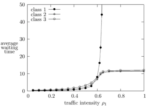
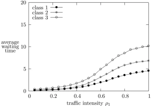
Average waiting times for classes 1, 2 and 3, as functions of traffic intensity

1

ρ _with ρ =₂ 0.5_and ρ =₃ 0.25₍_i.e._{, consistent with}_{Figure 3}_{) are shown in} Figure 4.

For ρ >1 0.25, queues 2 and 3 are nonstationary because their arrival rates

are greater than departure rates. Similarly, for ρ >1 0.571, queue 1 is

nonsta-tionary. In practical queueing systems the capacities of queues are finite, so the nonstationary regions correspond to dropping of some arriving packets because they cannot be queued.

If, however, the (constant) traffic intensities ρ2 and ρ3 do not exceed the

levels of traffic determined by the weights, the behavior of the queueing system is different, as shown in Figure 5 for ρ =2 0.25 and ρ =3 0.1.

In this case queue 1 becomes nonstationary at ρ1= −1 ρ2−ρ3=0.65.

(8)

[image:8.595.214.537.74.245.2] [image:8.595.252.495.291.463.2]

DOI: 10.4236/jcc.2018.611019 202 Journal of Computer and Communications Figure 2. Petri net model for class 1 of weighted priority queueing with a finite queue and weight 4.

Figure 3. Channel utilizations as functions of ρ1 with ρ =2 0.5 and ρ =3 0.25 for weighted priority queueing with infinite queues and weights 4-2-1.

[image:8.595.250.499.513.688.2]

(9)

[image:9.595.254.493.72.241.2]

DOI: 10.4236/jcc.2018.611019 203 Journal of Computer and Communications Figure 5. Channel utilizations as functions of ρ1 with ρ =2 0.25 and ρ =3 0.1 for weighted priority queueing with infinite queues and weights 4-2-1.

Figure 6. Average waiting times as functions of ρ1 with ρ =2 0.25 and ρ =3 0.1 for weighted priority queueing with infinite queues and weights 4-2-1.

When the capacity of a queue is finite, packets which arrive when the queue is full are dropped as they cannot be queued. The percentage of dropped packets is an important metric of the system. Figure 7 shows the fraction of packets which are dropped in a weighted priority queueing with weights 4-2-1 and with queue length equal to 5, as functions of traffic intensity ρ1 with ρ =2 0.5 and

3 0.25

ρ = .

Figure 7 shows that the fraction of packets dropped increases for ρ >1 0.25

and—for classes 2 and 3—reaches the level of 45% for ρ1 close to 0.6. This

should not be surprising because in the same range of values of ρ1 the

utiliza-tion of the shared channel decreases from 0.5 to 0.286 for class 2 and from 0.25 to 0.143 for class 3 (as shown in Figure 3). This decrease results is dropping about 45% of packets (practically the same for classes 2 and 3).

[image:9.595.251.496.286.463.2]

(10)

[image:10.595.255.495.72.241.2]

DOI: 10.4236/jcc.2018.611019 204 Journal of Computer and Communications Figure 7. Fraction of dropped packets as functions of ρ1 with ρ =2 0.5 and

3 0.25

[image:10.595.253.497.295.467.2]

ρ = for weighted priority queueing with queues length = 5 and weights 4-2-1.

Figure 8. Average waiting times as functions of ρ1 with ρ =2 0.5 and ρ =3 0.25 for weighted priority queueing with queue length = 5 and weights 4-2-1.

[image:10.595.252.492.516.689.2]

(11)

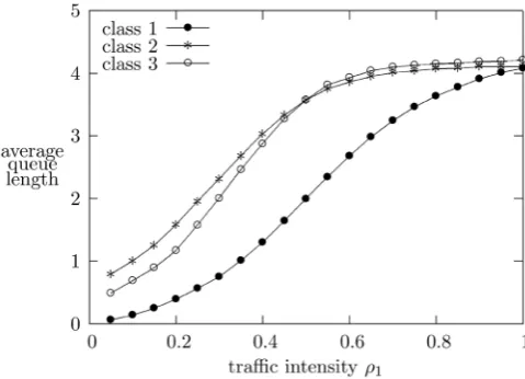
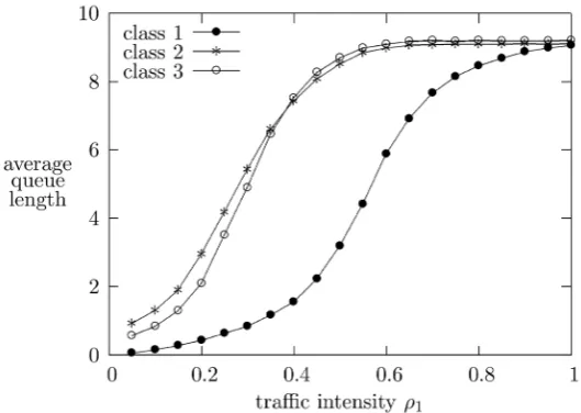
Results shown in Figure 7, Figure 8 and Figure 9 are related to each other. For weights 4-2-1 and for high-intensity traffic, each scheduling cycle includes 4 packets from class 1, 2 packets from class 2 and just 1 packet from class 3. Each packet served from class 3 is thus accompanied by 6 other packets, so if the av-erage length of the queue 3 is n, the average waiting time for class 3 is expected to be 7n. For n=4.2 (Figure 9), this results in the average waiting time for class 3 that is close to 30 (as shown in Figure 8). For class 2, two packets are served in each scheduling cycle, so its average waiting time is one half of that for class 3 (the average queue lengths are practically the same for classes 2 and 3, as shown in Figure 9).

It should be observed that from performance point of view, it is not beneficial to have long queues for packets waiting for service. For high intensity traffic these queues will be practically full, and then the average waiting time will simp-ly increase proportionalsimp-ly with the queue length. Figure 10 and Figure 11 show the average queue length and the average waiting time for the case when all queue lengths are equal to 10.

The average waiting times in Figure 11 are about two times greater than those in Figure 8.

Finally, Figure 12 and Figure 13 show the fraction of the dropped packets and the average waiting times for the case when the traffic intensities do not ex-ceed the levels determined by the weights, i.e., ρ =2 0.25 and ρ =3 0.1, as in Figure 6.

For class 1, the increase of the fraction of dropped packets is caused by queue 1 which is becoming full; all arriving packets which cannot be queued, are dropped.

[image:11.595.240.505.500.688.2]

For classes 2 and 3, the fraction of dropped packets is very small and the av-erage waiting times are also rather small.

(12)

[image:12.595.253.496.63.242.2] [image:12.595.249.496.292.464.2]

DOI: 10.4236/jcc.2018.611019 206 Journal of Computer and Communications Figure 11. Average waiting times as functions of ρ1 with ρ =2 0.5 and ρ3=0.25 for weighted priority queueing with queue length = 10 and weights 4-2-1.

Figure 12. Fraction of dropped packets as functions of ρ1 with ρ =2 0.25 and

3 0.1

ρ = for weighted priority queueing with queues length = 5 and weights 4-2-1.

Figure 13. Average waiting times as functions of ρ1 with ρ2=0.25 and

3 0.1

[image:12.595.248.500.515.690.2]

(13)

5. Concluding Remarks

Efficient use of modern networks requires detailed knowledge of network cha-racteristics, traffic statistics, transmission media types, and so on. Some of this information can be obtained by measurements performed under real traffic, but other can only be provided by detailed models, verified by comparisons with measurement data. On the basis of these characteristics, specific methods can be developed to determine the optimal numbers of links, the transmission capacity of links, the management strategy for resources shared among traffic classes, and others.

The goal of this paper is to provide insight into the behavior of weighted priority queueing, a modification of (strict) priority queueing that eliminates blocking of lower priority traffic that is typical for priority-based traffic man-agement schemes. The paper shows that when the weights match the characte-ristics of lower priority traffic, the performance provided by the analyzed scheme is actually quite good. However, since in real communication networks the cha-racteristics often change, a dynamic weight selection method may be needed for adjusting the performance to the changing character of the traffic. Some ideas for such a dynamic weighted queueing can be found in [15] and [16].

The weighted priority queueing exhibits several similarities to the weighted fair queueing [3], [17] but seems to be simpler to implement. An in-depth com-parison of these queueing methods is needed for better understanding their rela-tive strengths and weaknesses.

Conflicts of Interest

The authors declare no conflicts of interest regarding the publication of this pa-per.

References

[1] Giambene, G. (2014) Queueing Theory and Telecommunications—Networks and Applications. 2nd Edition, Springer-Verlag, New York.

[2] Georges, J.-P., Divoux, T. and Rondeau, E. (2005) Strict Priority versus Weighted Fair Queueing in Switched Ethernet Networks for Time Critical Applications. 19th IEEE International Parallel and Distributed Processing Symposium, Denver, 4-8 April 2005, 141-148. https://doi.org/10.1109/IPDPS.2005.413

[3] Dekeris, B., Adomkus, T. and Budnikas, A. (2006) Analysis of QoS Assurance Using Weighted Fair Queuing (WFQ) Scheduling Discipline with Low Latency Queue (LLQ). 28th International Conference on Information Technology Interfaces, Cav-tat/Dubrovnik, 19-22 June 2006, 507-512.

[4] Yang, L., Sheng, C., Zhang, E.-H. and Liu, H. (2012) A New Class of Priority-Based Weighted Fair Scheduling Algorithm. Physics Procedia, 33, 942-948.

https://doi.org/10.1016/j.phpro.2012.05.158

[5] Tannenbaum, A.S. (2003) Computer Networks. 4th Edition, Prentice-Hall, Engle-wood Cliffs.

(14)

System, 2, 118-121.

[7] Murata., T. (1989) Petri Nets: Properties, Analysis and Applications. Proceedings of IEEE, 77, 541-580. https://doi.org/10.1109/5.24143

[8] Reisig, W. (1985) Petri Nets—An Introduction (EATCS Monographs on Theoreti-cal Computer Science 4). Springer-Verlag, New York.

[9] Zuberek, W.M. (1991) Timed Petri Nets—Definitions, Properties and Applications.

Microelectronics and Reliability (Special Issue on Petri Nets and Related Graph Models), 31, 627-644. https://doi.org/10.1016/0026-2714(91)90007-T

[10] Allen, A.A. (1991) Probability, Statistics and Queueing Theory with Computer Science Applications. 2nd Edition, Academic Press, San Diego.

[11] Popova-Zeugmann, L. (2013) Time and Petri Nets. Springer-Verlag, Berlin Heidel-berg.

[12] Robertazzi, T.G. (1990) Computer Networks and Systems: Queueing Theory and Performance Evaluation. Springer-Verlag, New York.

https://doi.org/10.1007/978-1-4684-0385-5

[13] Zuberek, W.M. (1987) D-Timed Petri Nets and Modelling of Timeouts and Proto-cols. Transactions of the Society for Computer Simulation, 4, 331-357.

[14] Zuberek, W.M. (1986) M-Timed Petri Nets, Priorities, Preemptions, and Perfor-mance Evaluation of Systems. In: Advances in Petri Nets 1985, Springer-Verlag, Berlin, 478-498. https://doi.org/10.1007/BFb0016227

[15] Wang, H., Shen, C. and Shin, K. (2001) Adaptive Weighted Packet Scheduling for Premium Service. IEEE International Conference on Communications. Conference Record, Helsinki, 11-14 June 2001, 1846-1850.

[16] Panza, G., Graziolli, M. and Sidoti, F. (2005) Design and Analysis of a Dynamic Weighted Fair Queueing (WFQ) Scheduler. 15th IST Mobile and Wireless Com-munications Summit, Dresden, 19-23 July 2005, 134-138.

[17] Quadros, G., Alves, A., Monteiro, E. and Boavida, F. (2000) How Unfair Can Weighted fair Queuing Be? Fifth IEEE Symposium on Computers and Communica-tions (ISCC 2000), Antibes-Juan Les Pins, 3-6 July 2000, 779-784.