Selection of Bayesian single sampling plan for weighted Poisson distribution based on quality regions

(1)

RESEARCH ARTICLE

SELECTION OF BAYESIAN SINGLE SAMPLING PLAN FOR WEIGHTED POISSON DISTRIBUTION

BASED ON QUALITY REGIONS

*,1

_{Subbiah, K. and}

2

_{Latha, M.}

1

_{Research Scholar, Department of Statistics, Government Arts College, Udumalpet-642126, Tamil Nadu, India}

2

_{Principal, Kamarajar Government Arts College, Surandai- 627859, Tamil Nadu, India}

ARTICLE INFO ABSTRACT

This paper presents a new procedure for the construction and selection of Single Sampling Plan (SSP) using weighted gamma Poisson distribution as a base line distribution. The main theme from this article is to briefly present the theory and technique of (SSP) using Gamma prior distribution and demonstrate how it can facilitate to find Average Quality Level (AQL) and Limiting Quality Level

(LQL) bring about the result to reduce the Producer's Risk (α) and Consumer’s (β) Risk. In this

article, we further designs the parameter of the plan indexed with Probabilistic Quality Region (PQR) and Indifference Quality Regions (IQR) which gives potential application to improve the quality levels in industry products. Tables are constructed for the selection of plan parameters.

Copyright©2016, Subbiah and Latha. This is an open access article distributed under the Creative Commons Attribution License, which permits unrestricted use, distribution, and reproduction in any medium, provided the original work is properly cited.

INTRODUCTION

Acceptance Sampling uses sampling procedures to determine whether to accept or reject a product. It has been a common quality control technique that used in industry and particularly in military for contracts and procurement of products. Most often a producer supplies number of items to consumer and decision to accept or reject the lot is made through determining the number of defective items in a sample from the lot. The lot is accepted, if the number of defectives falls below the acceptance number (or) otherwise, the lot is rejected. A sample is taken and contains too many non-conforming items, then the batch is rejected otherwise it is accepted. Bayesian Acceptance sampling approach is associated with utilization of prior process history for the selection of distribution (viz. Gamma Poisson, Beta Binomial) to describe the random fluctuations involved in acceptance sampling. Bayesian sampling plans requires the uses to specify explicit the distribution of defectives from lot-to-lot quality on which the sampling plan is

*Corresponding author: Subbiah, K.

Research Scholar, Department of Statistics, Government Arts College, Udumalpet-642126, Tamil Nadu, India.

going to operate. The distribution is called prior because it is formulated prior to the taking of samples.

Bayesian Sampling inspection contains three components:

 The prior distribution (i.e.,) the expected distribution of submitted lots according to quality

 The cost of sampling inspection, acceptance (or) rejection

 A class of sampling plans that usually defined by means of a restriction designed to give a protection against accepting lots of poor quality.

The operating characteristic function is influenced by the plan parameters such as sample size (n), acceptance number (c) and the parameters of prior distribution is p. Analysis of OC function for different values of these parameters can determine range of the protection to both producer and consumer. This paper provides a new procedure for designing attribute single sampling plan indexed through ratios. Also considering the ability of the declination angles of the tangent at the inflection point on the OC curve for discrimination of the Single Sampling Plan (SSP).

ISSN: 0975-833X

International Journal of Current Research Vol. 8, Issue, 08, pp.36979-36984, August, 2016

INTERNATIONAL JOURNAL OF CURRENT RESEARCH

Article History: Received 17th_{May, 2016}

Received in revised form 20th_{June, 2016}

Accepted 17thJuly, 2016 Published online 31st_{August, 2016}

Citation: Subbiah, K. and Latha, M. 2016.“Selection of Bayesian single sampling plan for weighted Poisson distribution based on quality regions”,

International Journal of Current Research, 8, (08), 36979-36984. Key words:

Single sampling Plan, Bayesian Sampling plan, Average Quality Limit (AQL), Limiting Quality Limit (LQL), Producer's Risk, Consumer Risk, Indifference Quality Level (IQL), Probabilistic Quality Region (PQR), Indifference Quality Region (IQR), Quality Decision Region (QDR).

RESEARCH ARTICLE

SELECTION OF BAYESIAN SINGLE SAMPLING PLAN FOR WEIGHTED POISSON DISTRIBUTION

BASED ON QUALITY REGIONS

*,1

_{Subbiah, K. and}

2

_{Latha, M.}

1

_{Research Scholar, Department of Statistics, Government Arts College, Udumalpet-642126, Tamil Nadu, India}

2

_{Principal, Kamarajar Government Arts College, Surandai- 627859, Tamil Nadu, India}

INTRODUCTION

ISSN: 0975-833X

Citation: Subbiah, K. and Latha, M. 2016. “Selection of Bayesian single sampling plan for weighted Poisson distribution based on quality regions”,

Single sampling Plan, Bayesian Sampling plan, Average Quality Limit (AQL), Limiting Quality Limit (LQL), Producer's Risk, Consumer Risk, Indifference Quality Level (IQL), Probabilistic Quality Region (PQR), Indifference Quality Region (IQR), Quality Decision Region (QDR).

RESEARCH ARTICLE

SELECTION OF BAYESIAN SINGLE SAMPLING PLAN FOR WEIGHTED POISSON DISTRIBUTION

BASED ON QUALITY REGIONS

*,1

_{Subbiah, K. and}

2

_{Latha, M.}

1

_{Research Scholar, Department of Statistics, Government Arts College, Udumalpet-642126, Tamil Nadu, India}

2

_{Principal, Kamarajar Government Arts College, Surandai- 627859, Tamil Nadu, India}

INTRODUCTION

ISSN: 0975-833X

Citation: Subbiah, K. and Latha, M. 2016.“Selection of Bayesian single sampling plan for weighted Poisson distribution based on quality regions”,

(2)

Suresh and Latha (2001) has studied Bayesian single sampling plan through Average Probability of Acceptance involving Gamma Poisson model. Latha and Subbiah (2015) have studied the selection of Bayesian Multiple deferred state (BMDS-1) sampling plan based on quality regions. Calvin (1984) has provided procedures and tables for implementing Bayesian Sampling Plans. Hald (1965) has given a rather complete tabulation and discussed the properties of a system of single sampling attribute plans obtained by minimizing average costs are linear with fraction defective p and that the distribution of the quality is a double binomial distribution. Latha and Jeyabharathi (2012) has studied the selection of chain sampling attribute plan based on Geometric distribution.

Bayesian Single Sampling Plan

This paper related to Bayesian single sampling plan for Average probability function of incoming quality level.

Single Sampling Plan (SSP)

A single sampling plan is characterized by sample size n and the acceptance number c. sampling inspection in which the decision to accept or reject or not to accept is based on the inspection of a single sample size n.

Conditions for application of Single Sampling Plan:

 Production is continuous, so that results of the past, present and future lots are broadly the indicative of a continuous process.

 Lots are submitted sequentially.

 Inspection is by attributes, with the lot quality as the level defined as the proportion defective.

Operating Procedure:

Select a random sample of the size n and count the number of non-conforming units d. If there is c (or) less non-conforming units, the lot is accepted, otherwise the lot is rejected. Thus the plan is characterized by two parameters via, the sample size n and the acceptance number c.

The OC function of the single sampling plan is given as

Pa(p) = p(d≤ , ) (1)

The single sampling plan is characterized with sample size n and the ac-ceptance number c. The probability of acceptance of SSP based on weighted Poisson model is provided as

( )=∑ ( )

! , = 1,2,3…. (2)

Using the past history of inspection, it is observed that p follows a Beta distribution which is for convince approximated by a Gamma distribution (Hald,1981, pp. 133) with density function w(p)

= _Γ_{( )} , > 0 > 0 (3)

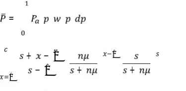
Thus, the average probability of acceptance is approximately obtained by

=

=∑

( , ) ( ) ( )

( ) x=1,2,3,….

=∑ (4)

where = is the first moment of the gamma distribution for

the product quality p.

Hence the above equation is Bayesian Single Sampling of Weighted Gamma Poisson distribution.

Selection o bayesian single sampling plan (BSSP)

Designing of quality interval BSSP (QIBSSP):

Quality decision region (QDR)

It is an interval of quality ( < < _∗) in which product is accepted at engineer's quality average. The quality is reliably maintained up to _∗ (MAPD) and sudden decline in quality is expected. This region is also called Reliable Quality Region (RQR). Quality decision range is denoted as d1= ( _∗− -1) is derived from the average probability of acceptance.

( < < _∗) =∑ ; <

< ∗ (5)

where = the mean value for the product quality p.

Probabilistic Quality Region (PQR)

It is an interval of quality ( < < ) in which product is accepted with a minimum probability 0.10 and maximum probability 0.95 probabilistic quality range denotes d2= ( − ) is derived from the average probability of acceptance.

( < < ) =∑ ;

< < (6)

Limiting Quality Region (LQR)

It is an interval of quality ( _∗< < ) in which product is accepted with a minimum probability 0.10 and maximum probability 0.95. Limiting quality range denoted as d3= ( − _∗) is derived from the average probability of acceptance.

( _∗< < ) =∑ ;

(3)

Indifference Quality region (IQR)

It is an interval of quality ( < < ) in which product is acceptd with a minimum probability 0.50 and maximum probability 0.95. Indifference quality range denoted as d0=( − ) is derived from the average probability of acceptance.

( < < ) =∑ ;

< < (8)

Selection of the sample plan

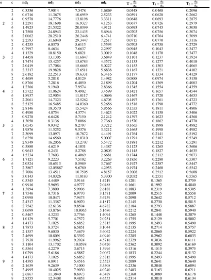
Table 1 shows the value of s ,m and corresponding ranges d1= nQDR, d2= nPQR, d3= nLQR and d0= nIQR. Define a ratio

T= ∗ = ∗ (9)

= ∗ ∗=

∗

∗ (10)

= ∗ = ∗ (11)

This is used to characterize the sampling plan. For any given values of QDR (d1), PQR(d2), LQR (d3) and IQR (d0). One can find the ratio T= , = , = . Find the value in

the table (1) under the column T,T1and T2, which is equal to or just less than the specified ratio, corresponding s and c, values are noted, from this ratio, one can determine the parameters for Bayesian single sampling plan.

Numerical Example

Given µ1=0.01,s = 5 and c = 2 compute the values of QDR,PQR,LQR and IQR. Then compute T, T1, T2 select the respective values from table 1. The nearest values are QDR=0.4980, PQR=4.8754, LQR=43774, IQR=1.4623 and the ratio T=0.1022, T1=0.1138, T2= 0.3406 with respect to s and c. Corresponding s and c, one can obtain the values of nµ1 from the table 2, which is nµ1= 0.3353. From this one can obtain n= = 0.3353≈33 using table 1. Thus the selected

parameters for bayesian single sampling plan are n=33, s=5 and c=2 (Bayesian single sampling plan (33,5,2)) through quality interval.

For specified QDR and PQR

Table (1) is used to construct the plans when the QDR and PQR are specified. For any given values of the QDR(d1) and PQR(d2), one can find the ratio, T= which is a monotonic

increasing function. Find the value in Table (1) under the column T which is equal to or just less than the specified ratio.

Then the corresponding values of s and c are noted. From this, one determines the parameters n, s and c for the Bayesian Single sampling plan.

Numerical Example: For a company 1 defects are seen in QDR and 9 defects are seen in PQR. Then d1 =0.01 and d2

=0.09, T1 = = 0.112. Find the ratio taking value 0.112.

Select value of T equal to or just less than this ratio using Table 1. The value of T is 0.1123 which is associated with s=6 and c=2. Also nd1 =0.05188, nd2 =4.62219, corresponding to s=6 and c=2. Thus n is calculated. The parameters for bayesian single sampling plan (56,6,2).

For specified QDR and LQR

Table 1 is used to construct the plans when the QDR and LQR are specified. For any given values of the QDR (d1) and LQR

(d3), one can find the ratio T1 = which is a monotonic

increasing function. Find the value in Table 1 under the column T1 which is equal to or just less than the specified ratio. Then the corresponding values of s and c are noted. From this, one determines the parameters n, s and c for the Bayesian Single sampling plan.

Numerical Example: For a company 1 percent defects are seen in QDR and 7 percent defects are seen in LQR. Then d1

=0.01 and d3= 0.07. T = = 0.143. Find the ratio taking

value 0.143. Select value of T1equal to or just less than this ratio using Table 1. The value of T1 is 0.1554 which is associated with s=4 and c=4. Also nd1=1.2366, nd3=7.9574 corresponding to s=4 and c=4. Thus n is calculated. The parameter s for the bayesian single sampling plan is (124, 4, 4)

For specified QDR and IQR

Table 1 is used to construct the plans when the QDR and IQR are specified. For any given values of the QDR(d1) and

LQR(d3), one can nd the ratio T1= which is a monotonic

increasing function. Find the value in Table (1) under the column T1 which is equal to or just less than the specified ratio. Then the corresponding values of s and c are noted. From this, one determines the parameters n, s and c for the Bayesian Single sampling plan.

Numerical Example: For a company 2 percent defects are seen in QDR and 8 percent defects are seen in IQR. Then d1

=0.02 and d0= 0.08. T2= = 0.25. Find the ratio taking values

0.25. Select value of T2 equal to or just less than this ratio using Table 1. The value of T2is 0.2662 which is associated with s=2 and c=3. Also nd1 =0.6716, nd0 =10.6959 corresponding to s=2 and c=3. Thus n is calculated. The parameter s for the bayesian single sampling plan is (34, 2, 3).

For specified AQL and LQL

(4)

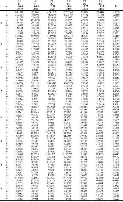
of m and nµ1 corresponding to the specified OR and s are found out. The sample size n is obtained by dividing µ1by µ. From this, one can determine the parameters n, s and c for the Bayesian single sampling plan.

Example:It is given that s = 3, at α = 0.05, µ1= 0.2% and β = 0.10, µ2= 4%. Then the operating ratio OR = = _. = 20.

The value of OR in table 2 nearer to 20 is 19.6040 for (nµ1) = 0.3245 and hence n is calculated as equal to .

[image:4.595.80.516.164.742.2]

. = 162.25≈ 162. The parameter for the Bayesian single sampling plan (162,3,2).

Table 1. Certain values of QDR, PQR, LQR, IQR and Operating characteristic ratio for specified values

s c nd1 nd2 nd3 nd0 _{T =} _T₁₌ _T₂₌

2

2 0.3536 7.9014 7.5478 1.6869 0.0448 0.0468 0.2096

3 0.6716 11.3675 10.6959 2.5233 0.0591 0.0628 0.2662

4 0.9578 14.7776 13.8198 3.3311 0.0648 0.0693 0.2875

5 1.2291 18.1698 16.9327 4.1253 0.0677 0.0726 0.2979

6 1.4923 21.5322 20.0399 4.9121 0.0693 0.0745 0.3038

7 1.7508 24.8943 23.1435 5.6946 0.0703 0.0756 0.3074

8 2.0062 28.2510 26.2448 6.4741 0.0710 0.0764 0.3099

9 2.2593 31.6040 29.3447 7.2517 0.0715 0.0770 0.3116

3

2 0.4255 6.0370 5.6115 1.5593 0.0705 0.0758 0.2729

3 0.7997 8.4634 7.6637 2.2997 0.0945 0.1043 0.3477

4 1.1329 10.8150 9.6821 3.0019 0.1048 0.1170 0.3477

5 1.4458 13.1305 11.6847 3.6849 0.1101 0.1237 0.3924

6 1.7474 15.4257 13.6783 4.3572 0.1133 0.1277 0.4010

7 2.0419 17.7084 15.6665 5.0227 0.1153 0.1303 0.4065

8 2.3317 19.9828 17.6511 5.6838 0.1167 0.1321 0.4102

9 2.6182 22.2513 19.6331 6.3416 0.1177 0.1334 0.4129

4

2 0.4689 5.2818 4.8129 1.4982 0.0888 0.0974 0.3130

3 0.8766 7.2816 6.4050 2.1899 0.1204 0.1369 0.4003

4 1.2366 9.1940 7.9574 2.8366 0.1345 0.1554 0.4359

5 1.5722 11.0624 9.4902 3.4599 0.1421 0.1657 0.4544

6 1.8937 12.9054 11.0117 4.0696 0.1467 0.1720 0.4653

7 2.2061 14.7323 12.5262 4.6705 0.1497 0.1761 0.4723

8 2.5125 16.5485 14.0360 5.2656 0.1518 0.1790 0.4772

9 2.8146 18.3570 15.5424 5.8566 0.1533 0.1811 0.4806

5

2 0.4980 4.8754 4.3774 1.4623 0.1022 0.1138 0.3406

3 0.9278 6.6428 5.7150 2.1242 0.1397 0.1623 0.4368

4 1.3050 8.3136 7.0086 2.7360 0.1570 0.1862 0.4770

5 1.6545 9.9342 8.2797 3.3212 0.1665 0.1998 0.4982

6 1.9876 11.5252 9.5376 3.3212 0.1665 0.1998 0.4982

7 2.3099 13.0971 10.7872 4.4491 0.1764 0.2141 0.5192

8 2.6250 14.6560 12.0310 5.0007 0.1791 0.2182 0.5249

9 2.9349 16.2056 13.2707 5.5472 0.1881 0.2212 0.5291

6

2 0.5880 4.6219 4.1031 1.4387 0.1123 0.1265 0.3606

3 0.9643 6.2431 5.2788 2.0803 0.1145 0.1827 0.4635

4 1.5334 7.7603 6.4069 2.6681 0.1744 0.2112 0.5073

5 1.7121 9.2223 7.5102 3.2263 0.1856 0.2280 0.5307

6 2.0524 10.6513 8.5989 3.7667 0.1927 0.2387 0.5447

7 2.3807 12.05887 9.6780 4.2953 0.1974 0.2460 0.5542

8 2.7006 13.4511 10.7505 4.8157 0.2008 0.2512 0.5608

9 3.0143 14.8326 11.8183 5.3300 0.2032 0.2551 0.5565

7

2 0.5345 4.4489 3.9144 1.4219 0.1201 0.1365 0.3759

3 0.9916 5.9693 4.9777 2.0488 0.1661 0.1992 0.4840

4 1.3894 7.3800 5.9906 2.6188 0.1883 0.2319 0.5305

5 1.7546 8.7316 6.9770 3.1571 0.2009 0.2515 0.5558

6 2.0998 10.0471 7.9473 3.6759 0.2090 0.2642 0.5712

7 2.4317 11.3387 8.9070 4.1817 0.2145 0.2730 0.5815

8 2.7542 12.6136 9.8594 4.6782 0.2184 0.2793 0.5887

9 3.0699 13.8764 10.8065 5.1680 0.2212 0.2841 0.5940

8

2 0.5467 4.3233 3.7766 1.4094 0.1265 0.1448 0.3879

3 1.0129 5.7701 4.7572 2.0251 0.1755 0.2129 0.5002

4 1.4173 7.1025 5.6852 2.5815 0.1995 0.2493 0.5490

5 1.7873 8.3724 6.5851 3.1044 0.2135 0.2714 0.5757

6 2.1357 9.6030 7.4679 3.6062 0.2224 0.2860 0.5922

7 2.4699 10.8091 8.3392 4.0940 0.2285 0.2962 0.6033

8 2.7938 11.9962 9.2024 4.5716 0.2329 0.3036 0.6111

9 3.1104 13.1702 10.0598 5.0420 0.2362 0.3092 0.6169

9

2 0.5564 4.2279 3.6715 1.3996 0.1316 0.1515 0.3975

3 1.0299 5.6186 4.5887 2.0067 0.1833 0.2244 0.5132

4 1.4173 7.1025 5.6852 2.5815 0.1995 0.2493 0.5490

5 1.4395 6.8911 5.4516 2.5523 0.2089 0.2641 0.5640

6 2.1639 9.2639 7.1000 3.5508 0.2336 0.3048 0.6094

7 2.4995 10.4025 7.9030 4.0240 0.2403 0.3163 0.6211

8 2.6867 11.3840 8.6973 4.3489 0.2360 0.3089 0.6178

(5)

[image:5.595.96.509.85.759.2]

Table 2.

s c α=0.05

β=0.10

α=0.05

β=0.05

α=0.01

β=0.10

α=0.01

β=0.05

α=0.25

β=0.10

α=0.25

β=0.05

h0

2

1 83.1654 133.5442 428.1782 687.5545 13.9774 22.4444 0.5858

2 26.2380 40.8096 65.6110 102.0487 8.4782 13.1866 0.7500

3 18.1792 27.9423 36.6856 56.3873 7.1662 11.0148 0.8277

4 15.1792 423.1858 27.7103 42.3265 6.5820 10.0538 0.8733

5 13.6334 20.7442 23.4977 35.7534 6.2516 9.5123 0.9034

6 12.6959 19.2669 21.0816 31.9928 6.0394 9.1652 0.9248

7 12.0681 18.2791 19.5249 29.5737 5.8915 8.9237 0.9408

8 11.6187 17.5730 18.4414 27.8922 5.7825 8.7459 0.9532

9 11.2811 17.0429 17.6433 26.6548 5.6989 8.6097 0.9631

3

1 66.6019 98.9096 342.9010 509.2376 11.4717 17.0364 0.6189

2 19.6040 27.9427 48.3764 68.9536 6.6052 9.4148 0.8277

3 13.0854 18.3516 25.8569 36.2630 5.4436 7.6343 0.9375

4 10.6813 14.8484 19.0032 26.4129 4.9245 6.8457 1.0064

5 9.4484 13.0613 15.8172 21.8654 4.6301 6.4005 1.0540

6 8.7028 11.9842 14.0020 19.2814 4.4402 6.1144 1.0888

7 8.2041 11.2654 12.8367 17.6267 4.3076 5.9150 1.1155

8 7.8474 10.7523 12.0279 16.4802 4.2097 5.7680 1.1367

9 7.5797 10.3677 11.4342 15.6398 4.1344 5.6551 1.1538

4

1 60.3314 86.4147 308.2277 441.4851 10.4361 14.9480 0.6364

2 16.9523 23.1824 41.5463 56.8150 5.8389 7.9847 0.8733

3 11.0658 14.8489 21.6176 29.0081 4.7389 6.3590 1.0064

4 8.9027 11.8209 15.6102 20.7271 4.2454 5.6369 1.0938

5 7.7959 1.2812 12.8339 16.9254 3.9646 5.2285 1.1560

6 7.1270 9.3546 11.2574 14.7759 3.7829 4.9652 1.2028

7 6.6796 8.7365 10.2473 13.4029 3.6558 4.7815 1.2393

8 6.3598 8.2960 9.5469 12.4533 3.5617 4.6460 1.2686

9 6.1199 7.9656 9.0339 11.7584 3.4892 4.5415 1.2927

5

1 56.6764 79.5116 289.5545 406.2178 9.8767 13.8561 0.6472

2 15.5404 20.7459 37.8960 50.5898 5.4244 7.2414 0.9034

3 9.9901 13.0620 2.1833 2.8546 4.3573 5.6971 1.0540

4 7.9570 10.2817 13.8206 17.8584 3.8771 5.0098 1.1560

5 6.9174 8.8701 11.2627 14.4421 3.6029 4.6200 1.2305

6 6.2890 8.0207 9.8126 12.5146 3.4252 4.3684 1.2875

7 5.8686 7.4544 8.8847 11.2854 3.3005 4.1923 1.3328

8 5.5682 7.0506 8.2419 10.4362 3.2080 4.0621 1.3696

9 5.3426 6.7481 7.7717 9.8162 3.1366 3.9618 1.4001

6

1 54.5010 75.4427 277.9010 384.6832 9.5243 13.1839 0.6546

2 14.6621 19.2678 35.6592 46.8605 5.1653 6.7878 0.9248

3 9.3241 11.9845 17.9910 23.1243 4.1184 5.2935 1.0888

4 7.3713 9.3549 12.7189 16.1415 3.6460 4.6271 1.2028

5 6.3727 8.0203 10.2953 12.9571 3.3758 4.2485 1.2875

6 5.7693 7.2179 8.9229 11.1633 3.2000 4.0035 1.3535

7 5.3656 6.6830 8.0461 10.0217 3.0765 3.8318 1.4065

8 5.0768 6.3014 7.4387 9.2331 2.9847 3.7047 1.4501

9 4.8598 6.0154 6.9943 8.6573 2.9138 3.6067 1.4865

7

1 52.9417 72.6000 269.9505 370.1881 9.2833 12.7303 0.6599

2 14.0658 18.2805 34.1125 44.3340 4.9879 6.4825 0.9408

3 8.8709 11.2648 17.0537 21.6558 3.9549 5.0222 1.1155

4 6.9728 8.7364 11.9728 15.0010 3.4877 4.3698 1.2393

5 6.0026 7.4543 9.6402 11.9717 3.2196 3.9983 1.3328

6 5.4159 6.6831 8.3214 10.2684 3.0451 3.7576 1.4065

7 5.0232 6.1690 7.4782 9.1839 2.9222 3.5887 1.4663

8 4.7420 5.8019 6.8946 8.4355 2.8308 3.4634 1.5159

9 4.5308 5.5267 6.4676 7.8892 2.7601 3.3668 1.5579

8

1 51.8097 70.5573 264.1782 359.7723 9.1096 12.4059 0.6640

2 13.6338 17.5739 33.0184 42.5605 4.8589 6.2631 0.9532

3 8.5436 10.7516 16.3784 20.6113 3.8358 4.8271 1.1367

4 6.6847 8.2955 11.4347 14.1900 3.3722 4.1848 1.2686

5 5.7347 7.0506 9.1680 11.2717 3.1057 3.8183 1.3696

6 5.1597 6.3014 7.8869 9.6319 2.9320 3.5807 1.4501

7 4.7749 5.8019 7.0681 8.5883 2.8093 3.4136 1.5159

8 4.4991 5.4451 6.5017 7.8688 2.7180 3.2895 1.5710

9 4.2920 5.1778 5.9679 7.1996 2.6473 3.1937 1.6179

9

1 51.0486 69.1556 259.7921 351.9406 8.9767 12.1608 0.6671

2 13.3047 17.0416 32.1710 41.2069 4.7610 6.0982 0.9631

3 8.2959 10.3674 15.8686 19.8308 3.7453 4.6804 1.1538

4 6.4670 7.9656 11.0291 13.5849 3.2843 4.0454 1.2927

5 5.5316 6.7479 7.5342 9.1909 3.0189 3.6828 1.4001

6 4.9655 6.0153 5.6289 6.8189 2.8456 3.4472 1.4865

7 4.5865 5.5267 4.7540 5.7285 2.7231 3.2814 1.5579

8 4.1506 4.9807 4.2511 5.1013 2.6318 3.1581 1.6179

(6)

Construction of Tables

The probability of acceptance of SSP based on weighted Poisson model is provided as

( )=∑ ( )₁ 1

!

1 , = 1,2,3….

= _Γ_{( )} , > 0 > 0

Thus, the average probability of acceptance P is approximately obtained by

=

+ − 2

− 1 +

1

+

1

Where = the mean value for the product quality p.

Table 1 shows the value of s and c corresponding ranges d1= nQDR, d2= nPQR, d3= nLQR and d0= nIQR from equation 5,6,7,and 8 and also represents operating characteristic ratio for specified values of s and c. Table 2 represents the conversion table, which is used to determine other quality characteristics.

Conclusion

Bayesian acceptance sampling is the technique, which deals with the producers in which decision to accept or reject lots or process based on their examination of past history or knowledge of samples. This paper deal with sampling model based on prior distribution and costs, which encompasses most of the existing Bayesian models based on costs. The work is presented in this paper mainly related to construction and selection Bayesian single sampling plan (BSSP) for Quality regions. Quality Interval Sampling (QIS) plan possesses wider potential applicability in industry ensuring higher standard of quality attainment for product or process.

Thus Quality Interval Sampling (QIS) plan is a good measure for defining quality and designing any acceptance sampling plan which are readymade use to industrial shop floor situations. The Quality Decision Region (QDR) idea is proposed in order to provide higher probability of acceptance compared with (AQL, LQL) indexed plan scheme. Quality Decision Region (QDR) depends on the quality on the quality measure MAPD, which is a key measure assessing to what degree the inflation point empowers the OC curve to discriminate between good and bad lots. The present development would be a valuable addition to the literature and a useful device for quality control practitioners. This paper mainly relates to the construction and selection of performance measures for Quality Interval Sampling (QIS) inspection plan indexed through quality regions.

REFERENCES

Calvin, T.W. 1984. How and when do perform Bayesian Acceptance Sampling Vol.7, American Society for Quality Control.

Hald, A 1981. Statistical Theory of sampling Inspection by Attributes, Academic Press London.

Latha, M and Jeyabharathi, S 2012. Selection of bayesian chain sampling attributes plans based on geometric distribution, International Journal of Scientific and Research Publication, vol.2,Issue 7, pp.1-8.

Latha, M and Subbiah, K. 2015. Selection of Bayesian multiple deferred state (BMDS-1) sampling plan based on quality regions, International Journal of Recent Scientific

Research, Vol.6, Issue 4, pp.275-282.

Lauer, N.G. 1978. Acceptance probabilities for sampling plans where the proportion defective has a beta distribution,

Journal of Quality Technology, Vol.3, Issue 4, pp. 275-282.

Mayer, P.L. 1967. A note on sum of Poisson probabilities and an application, Annals of institute of statistical Mathematics, Vol. 19,pp. 537-542.

Suresh, K.K. and Latha, M 2001. Bayesian single sampling plans for a Gamma Prior, Economic Quality Control, Vol.16, No.1, pp. 93-107.

[image:6.595.36.224.215.307.2]