Flexible GPBi CG Method for Nonsymmetric Linear Systems

(1)

http://dx.doi.org/10.4236/am.2012.34050 Published Online April 2012 (http://www.SciRP.org/journal/am)

Flexible GPBi-CG Method for Nonsymmetric

Linear Systems

*

Jia-Min Wang1, Tong-Xiang Gu2# 1

Chinese Academy of Engineering Physics, Beijing, China 2

Laboratory of Computational Physics, Institute of Applied Physics and Computational Mathematics, Beijing, China Email: #[email protected]

Received November 7,2011; revised February 22, 2012; accepted February 29, 2012

ABSTRACT

We present a flexible version of GPBi-CG algorithm which allows for the use of a different preconditioner at each step of the algorithm. In particular, a result of the flexibility of the variable preconditioner is to use any iterative method. For example, the standard GPBi-CG algorithm itself can be used as a preconditioner, as can other Krylov subspace methods or splitting methods. Numerical experiments are conducted for flexible GPBi-CG for a few matrices including some nonsymmetric matrices. These experiments illustrate the convergence and robustness of the flexible iterative method.

Keywords: Krylov Subspace Method; Flexible Preconditioning; Inner-Outer Iteration; GPBi-CG

1. Introduction

Krylov subspace methods are the iterative choice for solving linear system of the form

xb

A . (1) where the matrix A is assumed to be nonsingular. The strength of Krylov subspace methods are most apparent when combined with a preconditioner. We only consider right preconditioning in the paper. Thus one solves the equivalent linear system

 

1

M Mx b

A . (2)

The preconditioner M is selected to be close to the matrix A. And the matrix AM1 is never formed ex- plicitly. Instead, when M v1 z is needed, one solves the corresponding system

Mzv. (3) In this paper, we present a flexible version of GPBi- CG, which allows the preconditioner M vary from one iteration to another. Let us denote the matrix n the

preconditioner used in the nth iteration. The need to allow for a variable preconditioner arises when the solution of (2) is not obtained exactly (say, by a direct method), but is approximated by a second (inner) iterative method.

M

In recent years, several flexible variants of Krylov subspace methods have been established successfully. They

include flexible CG, which is applied on a symmetric positive definite matrix [1], flexible GMRES [2], flexible QMR [3], variable preconditioned GCR [4], flexible BiCG and flexible Bi-CGSTAB [5]. Preconditioning as this form is called flexible preconditioning, also known as variable or inexact preconditioning.

The paper is organized as follows. In the next section, we design the FGPBi-CG algorithm, which is a flexible version of GPBi-CG [6]. In Section 3, some numerical experiments will be conducted to illustrate the convergence of the algorithm. Furthermore, in some cases, it is shown that FGPBi-CG can achieve convergence to a tolerance when GPBi-CG is not convergent or even FBi-CGSTAB suffers stagnation. Finally we make some concluding remarks in Section 4.

Throughout the paper, x0 is the initial approximation,

0 0

r  b Ax is the initial residual, and the norm used is 2-norm.

2. Flexible GPBi-CG Method

We describe the basic idea of variable preconditioning and how it is incorporated with the algorithm GPBi-CG in this section.

The expression M v1

1

is calculated at each iteration of the conventional preconditioned Krylov subspace methods. The object of preconditioning is to change the original coefficient matrix A into another matrix close to identity, i.e. AM I . Consequently, the following property that _{M v}1

approximates _{A v}1

can be verified easily.

*_{The project is partly supported by the NSF of China (No. 61170309,}

No. 60973151, and No. 91130024) and the major project of scientific and technical development of China Academy of Engineering Physics (2011A0202012).

(2)

1 1

M v A v .

Thus, we consider obtaining an approximation of

1

A v instead of computing M v1 . That is, the following system (4) is roughly solved by an iterative method to a certain degree of accuracy that is not sufficient.

Azv. (4) Here, an approximation for the system (4) does not need to be solved at the same precision at each iteration. A stopping criteria has been established to make the preconditioner to be changed at each iteration. Different inner-loop can be applied to the system (4) including Krylov subspace methods and stationery iterative methods.

The GPBi-CG algorithm proposed by Zhang [6], uses an unified way to derive a class generalizations of Bi-CG. By choosing different coefficients, namely, the following

 and , the GPBi-CG algorithm will be reduced to other methods based on Bi-CG includes the well known CGS, Bi-CGSTAB, Bi-CGSTAB2.

Next we present a flexible version of GPBi-CG, which needs only some small modification of the GPBi-CG code.

ALGORITHM (FGP-BiCG with right preconditioner)

0

x is an initial guess, 0; is an arbitrary

vector, such that



, e.g., ; and set ,

0

r  b Ax



0,0 0 r r 

* 0 r * * 0 0 r r0

1 1 0

t w  1

1,

 ;

For n0, until rn  b do





1 1 1

n n n n n p  r   p u

solve M p_nˆp_n



*

 

*



0, 0, ˆ

n r rn r Ap

 

1 1 ˆ

n n n n n n

y t  r  w  Ap

ˆ

n n n

t  r  Ap

solve M tnˆtn































ˆ ˆ

, , , ,

ˆ, ˆ , , ˆ ,

n n n n n n n

n n n n

y y At t y t At y

ˆ

At At y y y At At y

  































ˆ, ˆ , , ˆ ˆ,

ˆ_, ˆ _, _, ˆ ˆ_, n n n n n

n n n n

At At y t y At At t At At y y y At At y

  



(if n0, then







ˆ,



, 0

ˆ, ˆ n

n n

At t At At

    )



1 1



ˆ

n n n n n n n

u  Ap t_  r  _u _₁

n

u

1

n n n n n n

z  r  z_ 

solve M z_nˆz_n

1 ˆ ˆ

n n n

x_ x  pz

1 ˆ

n n n n n

r_  t  y  A









* 0 1 * 0 , , n n n n n r r r r      ˆ ˆ n n

w At Ap

Enddo

at if we replace

Noted th Mn with M, a fixed precon-

di

erical experiments to tioner, the above algorithm e reduced to the standard GPBi-CG method with right preconditioner.

3. Numerical Experiments

will b

In this section, we report some num

show the convergence behaviors of FGPBi-CG. In all cases the iteration was started with x0 



0, 0,, 0



, and

the outer-loop is stopped when the relative residual norm

14 0 10

n

r r   . In the following examples, we use stopping criterion for inner-loop as:

1)  1

l

n k

r Az_  ;

2) The maximum number of iterations of inner loop

max

lN . Here, ( )1

l k

z_ denotes the l-th approximation when com-

t

puting Azv at k-th steps of the outer-loop.

3.1. Examples for Toeplitz Matrix

In the first example, we consider a Toeplitz matrix of order 200 with a parameter .

4 0 1 

 0.7 

4 0 1 0.7 4 0 1

4 0 4                           A 

In this experiment, we choose  to be 3.79 and the inner iteration stopping criteria to be the maximum iteration is Nmax 50 and relative residuals range from

3

10  _ 

to 106. We can see from the Figure 1 that GPBi-CG converges faster than that of Bi-CGSTAB. When the standard GPBi-CG algorithm performs well, the flexible version of GPBi-CG is also convergent, but it need more computation. The results can be seen in Table 1. In the table, “FG(B)” denotes FGPBi-CG with preconditioning Bi-CGSTAB, and so on, while “MV” represents the number of matrix-vector multiplication, “OIt” denotes the number of outer iteration.

[image:2.595.54.262.378.737.2] [image:2.595.360.488.424.512.2]

(3)

0 50 100 150 250 250 102

100

10–2

10–4

10–6

10–8

10–10

10–12

10–14

[image:3.595.63.286.85.258.2]

BiCGSTAB GPBiCG

Figure 1. Convergence history of Bi-CGSTAB and GPBi-CG for Toeplitz matrix 1.

[image:3.595.310.534.86.259.2]

(G)

Table 1. Performance comparison: γ = 3.79.

FG(B) FG(G) FB(B) FB



MV OIt MV OIt MV OIt MV OIt

3

10 550 3 506 3 356 3 316 3

4

10 454 2 416 2 294 2 258 3

5

10 1102 4 528 2 736 4 332 2

6

10 574 2 550 2 374 2 350 2

specti ely. Becau GPBi-CG se th n era n sually converges faster than Bi-CGSTAB.

v se u d in e in er it tio u

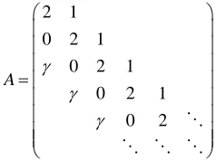
Now, we consider another Toeplitz matrix of order 200 with a parameter  as following.

2 1

0 2 1

 



0 2 1

0 2

A 

 

       

   

       

In this experiment, we choose  e th

to be 1.9 and the inner iteration stopping criteria to b e maximum itera- tio

CG is c gen hile Bi-CGSTAB is not. As a result, w

We consider the finite difference discretization of the par- n is Nmax50 and relative residuals range from

3 10

 _ 

to 106.

We can the Figure 2 and Table 2 that GPBi- onver t w

see from

hen Bi-CGSTAB is used as an inner iteration, the number of matrix vector multiplication is not influenced by the inner relative residual stopping criteria, i.e., the inner iteration is not terminated until it reaches Nmax (the

larg-est iterative number of inner loop). For this reason, GPBi- CG used as the inner iteration performs better.

3.2. Examples for Model Problem

0 100 200 300 400 500 600 700 800 900 1000 105

100

10–5

10–10

10–15

BiCGSTAB GPBiCG

Figure 2. Convergence history of Bi-CGSTAB and GPBi-CG for Toeplitz matrix 2.

[image:3.595.60.288.311.391.2]

FG(B) FG(G) FB(B) FB(G)

Table 2. Performance comparison: γ = 1.9.



3

10 3926 13 1158 5 2626 13 758 5

4

10 3926 13 904 3 2626 13 574 3

5

10 3926 13 896 3 2626 13 604 3

6

10 3926 13 906 3 2626 13 606 2

tial differentia equ ion ( ,5,7l at [3 ])



x y



u xu yu u

   f

     (5)

at the exact solution to the discretized equation

on a unit square, where f is such th

Axb is x



1,1,,1



. The parameters  and  are chosen to have a nonsymmetric matrix. In our experiment, 10 and  100

or  1000. The mesh is chosen of equal size in both dimension (32 nodes), and the corresponding matrix is thus of order 1024.

In the first example, we take  10,  100 and the inner iteration stopping criteria is N ranges from 30

max 6



.

3

to 70 and relative residuals is 10

For this choice, Figure 3 and Table show that both Bi-CGSTAB and GPBi-CG perform q well for this ex

uite

ample, flexible versions of these algorithms are also convergent. If the inner-loop stopping criterion is Nmax =

40 and  _₁₀6

, the FBi-CGSTAB(Bi-CGSTAB) needs 316 matrix vector multiplications to reach the prescribed tolerance, faster than that of Bi-CGSTAB.

In the next experiment, we choose 10,  1000

and the inner iteration stopping criteria is N ranges

fro s 10

max

m 90 to 1000 and relative residuals i .

Neither Bi-CGSTAB nor GPBi-CG witho t preconditioning is convergent for this problem (see F gu e 4).

9



u

i r

[image:3.595.113.232.455.544.2]

(4)

[image:4.595.148.443.86.319.2] [image:4.595.148.447.343.579.2]

Figure 3. Convergence history of Bi-CGSTAB and GPBi-CG for β = 10, γ = 100.

[image:4.595.60.289.619.733.2]

Figure 4. Convergence history of Bi-CGSTAB and GPBi-CG for β = 10 and γ = 1000.

Table 3. Performance comparison: β = 10, γ = 100. Table 4. Performance comparison: β = 10; γ = 1000.

FB(G) FG(G) FG(B) FG(G) FB(B) FB(G)

max N max

N

MV OIt MV O It

90

2534 7 9576 18

30 910 5 1274 7 482 4 488 4

40 446 2 726 3 316 2 486 3

50

60 484

498

2 520

2 512

2 334

2 350

2 348

2 358 2

2 14

170 2728 4 4

200

0 3372 6 6736 8

4088

3208 4 4808 4

300 4720 500

4 3

12,606 7972

7 3

1000

4836

4880 2 6870 2

[image:4.595.308.536.620.734.2]

(5)

CGSTAB, be ther are thr r-loops in the FGPBi-CG al m rat than t FBi-CGSTAB.

from able, we see FGPBi-CG (GPBi-CG c rges fo of t inner- stopping riteria. W appropriate stopp criteria is used in

4.

d to a certain degree of precision. In teration for solving Az = v is stopped

on Scientific C 4, 2000, pp. 1444-

cause e ee inne gorith her wo in

And this t )

1

onve r most he loop c

hen ing the inner

iteration, the flexible version will be a good choice.

Conclusion

We have formulated a flexible version of GPBi-CG for the large sparse nonsymmetric linear systems. The preconditioning is carried out by roughly solving Az = v by an iterative metho

our proposal, the i

according to satisfy a certain accuracy of approximation or the maximum number of iterations, so the preconditioner is changed at each outer iteration. Our numerical experiments show that FGPBi-CG is a viable alternative to GPBi-CG. And some examples show that FGPBi-CG is convergent when GPBi-CG suffers from stagnation.

REFERENCES

[1] Y. Notay, “Flexible Conjugate Gradients,” SIAM Journal

omputing, Vol. 22, No. 460. doi:10.1137/S1064827599362314

[2] Y. Saad, “A Flexible Inner-Outer Preconditioned GMRES Algorithm,” SIAM Journal on Scientific Computing, Vol. 14, No. 2, 1993, pp. 461-469. doi:10.1137/0914028 [3] D. B. Szyld and J. A. Vogel, “FQMR: A Flexible Quasi-

Minimal Residual Method with Inexact Preconditioning,” SIAM Journal on Scientific Computing, Vol. 23, No. 2, 2001, pp. 363-380. doi:10.1137/S106482750037336X [4] K. Abe and S.-L. Zhang, “A Variable Preconditioning Us-

ing the SOR Method For GCR-Like Methods,” Interna- tional Journal of Numerical Analysis and Modeling, Vol. 2, No.2, 2005, pp. 147-161.

[5] J. A. Vogel, “Flexible BiCG and Flexible Bi-CGSTAB for Nonsymmetric Linear Systems,” Applied Mathematics and Computation, Vol. 188, No. 1, 2007, pp. 226-233. doi:10.1016/j.amc.2006.09.116

[6] S.-L. Zhang, “GPBi-CG: Generalized Product-Type Meth- ods Baseed on Bi-CG for Solving Nonsymentric Linea Systems,” SIAM Journal on Sc

r ientific Computing, Vol. 18, No. 2, 1997, pp. 537-551.

doi:10.1137/S1064827592236313

[7] Y. Saad, “Iterative Method for Solving Linear Systems,” 2nd Edition, SIAM, Philadelphia, 2003.